Statistical Analysis of Annual Flood Series and Partial Duration Series.

Author Role:

Title, Monographic: Statistical analysis of annual flood series and partial duration series Translated Title:

Reprint Status: Edition:

Author, Subsidiary: Author Role:

Place of Publication: Québec Publisher Name: INRS-Eau Date of Publication: 1985

Original Publication Date: Février 1985 Volume Identification:

Extent of Work: 123

Packaging Method: pages Series Editor:

Series Editor Role:

Series Title: INRS-Eau, Rapport de recherche Series Volume ID: 177

Location/URL:

ISBN: 2-89146-175-4

Notes: Rapport annuel 1985-1986

Abstract: 20.00$

Call Number: R000177 Keywords: rapport/ ok/ dl

by

Fahim Ashkar and Bernard Bobêe Rapport scientifique # 177 INRS-Eau February, 1985

1.

2.

PAGE

FUNDAMENTAL CONCEPTS 2

1.1 Annual Series and Partial Duration Series 2

1.2 The Return Period as Measure of Risk 4

1.3 A Reliability Criterion for Flood Flow Estimates 11

1.4 Mixed Polulations 12

1.5 Plotting Position 14

SINGLE SITE ANALYSIS 18

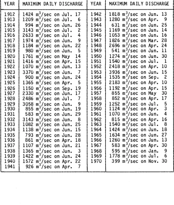
2.1 Data Base 18

2.1.1 Introduction 18

2.1. 2 Conditions Reguired from the Data 18 2.1. 3 Random Variables and their Statistical

Characteristics 28

2.1.4 Methods of Estimation 30

2.1.5 Sampling Variances and Confidence Intervals 37 2.2 Common Probability Distributions and fitting

Techniques 44

2.2.1 Introduction 44

2.2.2 The Normal Distribution 45

2.2.3 The Lognormal Distribution 46

2.2.4 The Gumbel Distributin (Type 1 Extermal) 52 2.2.5 The Pearson Type 3 Distribution 58

Freguency Distributions 73

2.2.8 ExamEle of AEElication 78

2.2.9 Conclusion 83

2.3 Partial Duration Series Models 86

2.3.1 Mathematical Presentation 86

2.3.2 Estimation of Design Events and Uncertainty

of Estimation 94

2.3.3 ComEarison of Annual Series and Partial

Duration Series 97

2.3.4 Treatment of Non Identically Distributed

Exceedances 98

2.3.5 AEElications and Additional Comments 103

REFERENCES 113

TABLES 118

1. FUNDAMENTAL CONCEPTS

The analysis of flood probability distributions plays a major rol e in hydrologie and econorni c eval uations of water resources projects and in establishing project design criteria. In general, one wishes to determine a statistical distribution or a probabi-l ity modeprobabi-l suitabprobabi-le for representing a sampprobabi-l e of run-off fprobabi-lows. With such a distribution or such a model it then becomes possible to estimate events corresponding to a given probability. These estimations are basic for the construction works and help to permit an efficient design.

1.1. Annual Series and Partial Duration Series

Starting with a recorded hydrograph or with the tabulated data abstracted from thi 5 hydrograph, two types of flood peak series may be used in a frequency analysis. These are the annual flood series (a.f.s.) which consists of the largest flood in each year, and the partial flood series (p.f.s.) which consists of all "well-defined" flood peaks above a specified magnitude, often called the flood truncation level or base level. In fact one of the drawbacks of partial flood series (also called partial dura-tion series; p.d.s.) is that it is not completely well-defined which of the flood peaks exceeding the base level should be retained for the analysis and which should be excluded. Since in p.d.s. models now in common use, it is required that sucessive

flood peaks shou1d be independent, sorne flood investigators (Cun-nane, 1979; Water Resources Counci1, 1976, and others) have propo-sed putting restrictions on the inter-arriva1 times of flood events (flood peaks) so that these events wi 11 not occur close together in bunches. Water Resources Counci1 (1976) arbitrari1y defined separate flood events as events separated by at 1east as many days as five plus the natura1 10garithm of square miles of drainage area, with the requirement that the intermediate f10ws must drop be10w 75 percent of the 10wer of the two separate maxi-mum daily f10ws. Todorovic and Zelenhasic (1970) and Todorovic and Rousselle (1971) defined the partial flood series as al1 flood peaks ab ove the base level, and in the case of a mu1tip1e-peaked flood hydrograph only the largest discharge is considered as the flood peak to be retained. This is done with the expectation that when the base level is sufficiently high the independence of flood peaks (al so called exceedances) woul d become physically pl ausi-ble.

Although annual flood series are more precisely defined than partial flood series they have the disadvantage that they use on1y one flood per year. In certain cases the second largest flood in a year may outrank many annua l floods of other years and yet i t i s totally neglected in the a.f.s. approach. This disadvantage is remedied in the p.d.s. approach in which the truncation level is generally selected low enough that the average number of exceedan-ces per year is of the order of two or three.

1.2. The Return Period as a Measure of Risk

Langbein (1949) and Chow (1950) investigated the theoretical relationship between the probability of annual flood series and the expectancy of partial flood series. Let P be the expectancy

p

of a variate in the partial flood series being equal to or greater th an x, and let m be the average number of events per year, or mN be the total number of events in N years of record. Th en P p/m i s the annual probability of an event being equal to or greater than x, and 1 - P /m i s the probab il i ty of an event bei ng 1 ess

p

than x. The probabil ity of an event x being the 1 argest of the

m

m events in a year would then be (1 - pp/ml • This probability can be approximated by exp (- P ) when Pis small compared

p p

with m. Note also that this is the probability of an annual event of magnitude x and corresponds to the annual series. Hence, the probability Pa of an annual flood series of magnitude x being equaled or exceeded is:

P

=

1 - exp (- P )

a p

P

= -

ln Cl - p )

p a (1.1 )

The time el apsi ng between successive events of magnitude equalling or exceeding a specified value x is a random variable whose mean value is defined as the return period T of x (notation: T = T(x) or T = T). Al ternative1y, each flood value x may be

x

considered as a function of its associated value of return period (notation: x

=

x(T) or x

=

x

T). The return periods of annua1 series and partial duration series have different meanings. In the first case the return period T is the mean recurrence time of

a

an event of a given magnitude as an annua1 maximum whi1e in the second case the return period Tp carries no implication of annua1 maximum.

Letting T

=

l/P and T

=

l/P in equation (1.1) yie1ds:

a a p p

1

T

_{P ---}

=

lnTa -ln(Ta-1)

(1. 2)

from which it can be seen that T , the return period in partial

p

flood series is sma11er than Ta in annual series but that T_p approaches T as both T and T increase. Langbein (1949) states

a p a

that the difference between T and T becomes negligible for

floods greater than about a five-year return periode

Equation (1.2) is an approximate relationship because it is based on approximating (1 - pp/m}m by exp (- Pp). An alternative derivati on of rel ati onshi p (1. 2) was presented recently by Takeu chi (1984) who reconfirmed its validity and encouraged its practi-cal use.

The definition we have just given for the return period T

p

for partial duration series can be modified to carry more implica-tion of annual maximum. Let Xl' X2' ••• , X_{n be the sequence of}

annual maximum values abstracted from a partial flood series. This means that if the year i contains no exceedances or no flood peaks above the base level Xo then the value of xi for that year will be equal to zero, when the discharge Xo is taken as reference (base 1 evel) • In other words, if the year j contains mjexceed-ances ~l' ~2' ~mj then: X j

=

1

max

(~l'

o

for m. J ~ 2 , ••• , ~mj) for m j > 0

=

0 (1.3 )

exceed-ing xo simp1y by subtractexceed-ing xo: ~i

=

Qi - xo. If the distribu-tion of the ~.s and of the m.s is known, then the distribution of

1 J

the Xjs can be deduced and the probabi1ity of the variable ~

equa11ing or exceeding a specified magnitude x can be ca1cu1ated. If this probabi1ity is now denoted by P (the subscript p standing

p

for IIp.d.s.") then T

=

1/P wou1d be the new definition of the

p p

return period for partial duration series. This definition, which is more convenient for mathematica1 treatment than the previous one, i s the one in common use [see for instance Todorovi c and Ze1enhasic 1970, Todorovic and Rousselle 1971, Ashkar and Rousselle 1981]. We sha11 make no further reference to the previous definition of T in the rest of our discussion. The new

p

definition of T_p is nearer to the definition of Ta given for the annua1 series but still differs from it because the term lIannua1 maximum Il does not carry the same meaning in a.f.s. as in p.f.s.

On 1y years that produce a peak di scharge superi or to the base discharge yield the same value of annual maximum for a.f.s. as for p.f.s. In general, therefore, we expect that the higher the average number of exceedances per year, the nearer Ta and Tp are to each other.

Lloyd (1970) considered the exceedance probabi1ity P [X > ~]

associated with an arbitrary random variable X and a return period

1 p [X > XT]

=

P

=

-T

(1. 4)

and showed that T, as a random variable, has a distribution of the form:

P [T

=

t]

=

p (1 _ p) t-1 _{(1. 5)}

This distribution has for mean and variance:

mean E(T}

=

l/p

variance: Var (T) = (1 - p}/p2

If a period of r years is considered, the probability P that the event X > x

T will occur at least once during these r years is P

=

1 - Q, where Q is the probability of not having a flow X > x

T during r years. This gives

1

r r

P

=

1 - (1 - p)

=

1 - (1 - -) (1.6 )

which can be written as

1

T

=

-1 - (1 _ p )l/r

(1. 7)

This expression can also be written in an approximative form:

The following simple applications of relationships (1.6) and (1. 7) are i ntended to hel p better understand the concepts of return period and of reciprocal probability.

Applications

(1) Considering a return period of T

=

100 years, the probability P that duri ng these 100 years to come, the centenary flow (p

=

0.01) will be exceeded at least once, is

P

=

1 - (1 - 0.01)100

P

=

.63

There is therefore a 63 % chance that the centenary flow will occur during the 100 years to come.

(2) One wishes to construct a public work having a duration life of r

=

50 years and one wishes to determine the return period T such that the flow X > x

T wi 11 occur wi th a probabil ity less than or equal to 20 %. Thus

T

> 50

(_1 __

0.5) .20

T > 225 years

The work must thus be constructed so that the return period T

=

225 years if one wishes that in the 50 years to come, the flow X > x

T will occur with a probability less than or equal to 20 %.

In this last example, the probability 20 % that one or more events will exceed a given flood magnitude (the flood correspond-ing to a return period of 225 years) within a specified number of years (50 years) i s sometimes referred to as the Il ri sk

ll

associ ated with the given flood magnitude and with the specified number of years. For a one - year period, the probability of exceedance p, which is the reciprocal of the recurrence interval T, expresses this risk. Table 1.1 gives for different return periods T the percent chance (risk) of getting one or more floods of return period T, or greater, within one of a number of different lengths of time.

1.3. A Reliability Criterion for Flood Flow Estimates

The reliability of flood flow estimates obtained from the recorded data by extrapolation is directly related to the length of record. The following criterion is proposed by Hardison

(1969) : ( Number of years of

1

Maximum recurrence data collection interval 2 5 10 15 20 25 years 2 5 10 15 50 100 years

Hardison (1969) has shown that this criterion gives sufficiently close estimates for xT.

1.4. Mixed Populations

In areas where hi gh flows are generated by more th an one distinct hydrologie process (e.g. snownelt - and rainfall - gen-erated peaks), peak di scharge data shoul d be consi dered to be drawn from subpopulations with different statistical characteris-tics. Stoddart and Watt (1970) for exampl e have described how flooding in sorne watersheds in southern Ontario is created by two different types of events. In these watersheds rain floods occur generally in the summer and floods due to snownel t, sometimes combined with precipitation, occur in winter and spring. Waylen and Woo (1982) describe also how floods in the Cascade Mountains of southern British Columbia can be due to heavy winter rainfall, or snowmelt in spring.

When i t can be shown that floods on record come from two or more distinct populations then it may be more hydrologically reasonable to try to find to what subpopulation each flood belongs and then to analyse each subpopul ati on separately, rather than separating floods by calendar periods. This, unless of course, the events in the separate periods are clearly caused by different hydrometeorologic conditions.

Consider two independent flood generating processes, a and b say, and suppose that a flood of a given magnitude x would have a return period Ta if it belongs to population a and Tb if it

belongs to population b. The probabilities of not exceeding x are

q

=

1 - l/T

a a

and

The probability of not exceeding x in any year becomes

and the return peri od for the annua 1 flood associ ated wi th the level x becomes

or

T

=

T T / (T + T - 1)

a b a b (1.8)

1.5 Plotting Position

In frequency analysis of hydrological data a statistical model may be postul ated whose parameters are estimated from the observed data (cf. section 2.1.4), or alternatively, an empirical distribution of the observed magnitudes may be obtained by graphical analysis on a probability plot. In the latter method the ranked data are plotted on probability paper using probability as abscissa values obtained from a plotting position formul a. This plotting may help in getting a better interpretation of the data, in detecting any possible errors, or in picking an adequate probability distribution for fitting the data. The scale of the abscissa is frequently arranged in such a way that events distri-buted according to a given probability distribution will plot as a straight line.

Numerous works have been produced on the subject of plotting position both because of the practical importance of the choice of this empirical probability and because there is no formula which is entirely satisfactory in finding it. Gumbel (1958) states four

postulates which the plotting position Pk of the event of order k of an ordered sample (Xl> ••• > X

k > ••• > xN) must satisfy:

(1) the plotting position shoul d be such that all observations can be plotted;

(2) the plotting position should be between the observed frequen-cies (k - 1) / N and k/N and should be distribution free;

(3) the return peri od of a val ue equal to or 1 arger than the largest observation should approach N, the number of observa-tions;

(4) the observations shoul d be equally spaced on the frequency scale, i.e. the difference between the observations of order (k + 1) and k should be a function of N only and be indepen-dent of k.

Among the principal formul as currently found in practical use, the following may be cited:

k - 0.5

p

=

k

-N

This formula is recommended by Brunet-Moret (1973) for the case where the parameters of the adjusted distribution are estimated from the sample.

The Wei bull formul a:

k

p

=

k -N-+-1

This formula is recommended by Chow (1953) for the study of flows. It is the average of the probabilities of all events with rank k in a series of periods, each of N years.

The Chegodayev formula:

k - 0.3

p

=

This formula is recommenaed by Kimball (1960) as well as by Brunet-Moret (1973) for the case where the parameters of the distribution are known a priori. Th i s formul a gives the approximate probability of the median of the distribution of the statistic of order k from a sample of size N.

A critical review of Gumbel ' s postul ates has been given by Cunnane (1978) who argued against postulate (3), notably that the

return peri od of a val ue equal to or greater than the 1 argest observation should converge towards N, the number of observations. Hi s argument was based on statistical properties of the 1 argest value in a sample of size N. He proposed a plotting position that has the property that quantile estimates made from the plot will be unbiased and will have smallest mean square error among all suc h est i mat es. Th i sun b i as e d plo t tin 9 po si t ion i s n am e 1 y E (y(i)) the mean of the ith order statistic in samples from the reduced variate population. E (Y(i)) has the disadvantage, however, that it depends on the form of the distribution being considered, and if the reduced variate depends on a shape parameter then E (y(i)) too depends on this parameter.

2. SINGLE SITE ANALYSIS

2.1. DATA BASE

2.1.1. Introduction

In flood frequency analysis, the primary objectives are to determine the return periods of recorded events of known magnitu-des and then to estimate the magni tude of events for return periods beyond the recorded range, that can be used in the design of hydraulic structures and the planning and management of water resources systems. In this kind of analysis it is important to try to abstract the maximum information from the available data. Inadequate estimations may come from:

- the use of inadequate data;

- the wrong choice of a representative statistical distribution;

- the inadequate use of a technique for estimating the parameters of the chosen law.

For these reasons we shall be dealing in the remainder of secti on 2. wi th:

- conditions that are required of relevant data before the appli-cation of a statistical distribution;

- the characteristics of the distributions habitually used to represent run-off flows;

- properties and particularities of the principal methods of estimating parameters.

2.1.2. Conditions Required from the Data

Before one may adjust a statistical law to a given sample it must be demonstrated that the elements of this sample verify three conditions:

A. temporal independence; B • homogene i ty;

C. stationarity.

A. Condition of temporal independence

To estimate the probabilities of hydrologie events, one assumes generally that the observed flows are independently distributed in time. Streamflow sequences, however, tend to be persistent in that high flows tend to follow high flows and low flows tend to follow low flows. This persistence depends on the

lapse of time separating the successive elements of the sequence; dependence among successive daily flow values, for instance, tends to be strong, while dependence among yearly values, is weak.

The independence of the sample elements of flood flows can be checked using either the Wald and Wolfowitz (1943) test or the Anderson (1941) test.

Wald and Wolfowitz test

For a sample of size N (Xl' ••• , X_N) we consider the

statis-tic R such that

N-l

R

=

I

xi xi+l + xl XN i=l

In the case where the el ements of the sampl e are i ndependent, R follows a normal distribution with mean and variance given by

_ 2

R

=

(s - S2) / (N - 1)

Var (R) 2 _ 4

=

(s - S4) / (N - 1) - R2 + (s 2 1 2 2 - 4s S2 1 + 4 SIS 3 + S - 2 S 4) / (N - 1) (N - 2) 2 th

where rn_r is the r moment of the sample about the origin (cf. section 2.1.4 A).

The quantity u

=

(R -

R) /

(var R)I/2 follows a standardized normal distribution (mean 0 and variance 1) and can be used to test the hypothesis of independence.

Anderson test

Let rI be the first-order serial correlation of the sample given by

x·

2

For a normal random time series of N values, rI is nearly normally distributed with a mean: rI

= -

1 / (N - 1) a variance: Va r rI

=

(N - 2) / (N - 1) 2

-Considering the quantity u

=

(rI - rI) / (var rdl/2 _{it is} possi-ble to test whether rI at a given level is significantly different from zero. Al though thi s test i s only theoretically val id for samples taken from a normal distribution, it is generally used for other parent populations also.

B. Condition of representativeness of the sample

The condition of representativeness impl ies that all the elements of the sample originate from the same population. In annual flood series as well as in partial duration series it may happen that the sample is composed of events of different origin belonging to different populations (e.g., sno\\ffielt and rainfall fl oods) • To check whether two samples belong to the same popul ation we can use the Terry (1952) test or the Mann and Whitney (1947) test.

Terry test

Given two samples of size p and q, respectively, the combined set of N

=

P + q observati ons i s ranked in i ncreasi ng order. If in the complete series I denotes the ranks of the elements of the first sample and J those of the observations of the second sample, we consider the statistic C given by

C

=

l

E (X

J N)

J '

where E (X

k

,

N) denotes the mathematical expectation of the kth-order statistic in a sample of size N from a standardized normal

popul ation.

For N > 15, under the null hypothesis that the two sampl es belong to the same population, the quantity

with

t

=

C [(N - 2) / [(N - 1) var C - C2JJl/2

N

Va r C

=

(pq / N (N - 1))·

l

E 2 (X k ,N ) k=1

follows approximately a Student distribution with (N - 2) degrees of freedom. In practice, the values of E (X

k

,

N) may be obtained from the Harter (1961) tables.

Mann-Whitney test

As was done above, we regroup two sampl es of size p and q (with p < q) in a combined set of size N

=

P + q, ranked in

v =

T - p (p + 1) / 2

W

=

pq - V

where T i s the sum of the ranks of the el ements of the fi rst sample (of size p) in the combined series and V is the number of times that an item in sample 1 follows in the ranking an item in sample 2; W is computed in a similar way for sample 2 following sample 1.

When N > 20, p, q > 3, and under the null hypothesis that the two sampl es come from the same popul ation, V and W are approxi-mately normally distributed with mean pq / 2 and variance pq (p + q + 1) /12. In practice we consider the quantity

v -

pq / 2

u

= ____________________ _

[pq (p + q + 1) / 12]1/2

and for a test at a level of significance u, u is compared with the standardized normal variate corresponding to a probability of

u exceedance -.

In practice, to study the run-off flows at a given station, one can consider the sample fonned from the maximum annual flow (or the sample formed from the exceedances, in the p.d.s. approach) duri ng N years and exami ne the i ndependence of the elements of the sample. If however, the flows are due to two different causes, for example a flow due to snowmelt which occurs in the spring and the autumn flows due to over-abundant precipita-tion, it is possible to test for heterogeneity between the two sampl es. In the case where there i s heterogenei ty, i t i s reason-able to consider the two types of flow separately.

For an application of tests of independence and of homogene-ity refer to the example given in section 2.2.8.

C. Condition of stationarity

The assumpti on that the natural processes i nfl uencing river flow characteristics are stationary with respect to time is diffi-cult to guarantee. Non-stationary behaviour may occur in a number of different forms. There are the slow changes in hydrologie parameters and the rapid changes. An example of the slow changes are evol uti onary changes such as gradual movements in cl imate, involving for instance, increasing or decreasing rainfall. Urbanization and variations in catchment characteristics are another form of slow change. Rapid changes may resul t, for instance, from earthquakes or from building of dams.

In current hydrologic investigations, the problem of exis-tence of long term variations, conceived as fluctuations of the basic characteristics of hydrologic time series, in function of time, is one of the most controversial problems. The question at stake, is whether or not, trends, periodicity, or other non-stationarity in the probability structure of hydrologic time series beyond the periodicity of the year, do really exist. Existing techniques of time series analysis cannot answer this question. Based on sorne studies which do not support the concept of non-stationarity in hydrologic series of annual values (see Yevjevich, 1963 for instance) we shall make the conventional assumption that no non-stationarity exists in hydrologic series, beyond the periodicity of the year.

Flood records used in frequency analysi s shoul d represent relatively constant watershed conditions. The records shoul d be carefully examined to make sure that no major changes within the wa tershed have occurred duri ng the peri od of record si nce such changes effect record homogeneity. Tests discussed in the previous paragraph can be used to check for any significant nonhomogeneity when it is suspected that such a nonhomogeneity in flood values might be present.

2.1.3. Random Variables and their Statistical Characteristics

From a fai rly short record of streamfl ow, how does one estimate a design flood? As we mentioned earl ier, thegeneral approach is to use the sample data to fit a frequency distribution which in turn is used to extrapolate from the recorded events to the design events. The first step consists of choosing a frequen-cy distribution. Subsequently, the parameters of this distribu-tion are estimated and used to extrapolate beyond the domain of recorded events.

Given a sample of independent hydrologie observations Xl, X2, " ' , xN let X be the random variable (r.v.) representing the population from which this set of observations is drawn. If the population consists of an infinite set of elements distributed over an interval D of finite or infinite length then we have what is called a "continuous population" which may be represented by:

its continuous probability density function (p.d.f.) f (x;

°

_{1 , " ' ,} Ok) where _{8 1 , "" 8k are parameters;}

- its continuous cumulative distribution function (usually called simply "distribution function") defined as:

x

F (x)

=

P [X < x]

=

f

f (x) dx _00

which means that

dF (x)

f (x)

= _ _

_

dx

While most of the probability distributions used in flood frequency analysis are of the continuous type, sorne distributions, such as the Poisson distribution used in partial duration series model s to represent the number of flood exceedances in an arbi-trary but fixed interva1 of time (section 2.3.1) are not contin-uous. The Poisson distribution which can asslJl1e the discrete values 0, 1, 2, ••• is a member of the class of "discrete distri-butions" which can assume values over a finite or infinite set S of di screte or separate val ues. If i i s an el ement of the set S then the discrete random variable X defined over S may be repre-sented by:

- its discrete probabi1ity density function (a1so called mass function) f (i; G_{l ,} ••• , Gk)

=

P [X

=

iJ where Gb ••• , Gk are parameters;

- its (cumulative) distribution function defined as

F (i)

=

P [X < i]

=

l

f (j) jES;j<i

2.1.4 Methods of Estimation

Several methods for the estimation of parameters of a (con-tinuous or discrete) p.d.f. are available and are more or less adequate depending upon the distribution chosen. The two princi-pal methods of estimation used in practice are:

- the method of moments;

- the method of maximum likelihood.

A. Method of moments

For a given distribution, depending on k parameters it is possible to calcul ate the non-central and central moments about the mean. This gives the non-central moment of order r, jJr such that:

jJ _r

=

J

xr f (x) dx

and ~r the central moment of order r around the mean ~1 such that:

1 r

~

=

f

(x - ~1) f (x) dx

r D

The variate

X

defined over the interval

D

has probability density function f (x). In the case of a discrete random variable the integration over D is replaced by a summation over the set S over which the discrete r.v. is defined.

Si nce f (x) depends on the parameters 01, ••• , Ok' the moments ~ _r and ~ _r are functions of the parameters. These moments can be estimated numerically by means of the corresponding sample moments. For a sample Xl, ••• , xN the non-central sample moment of order r, mr is given by:

1 N

l

x~ N i=l 1

i s given by: 1 N mr

= -

l

N i=l - r (x. - x) 1

where N is the size of the sample.

Thus, for a law of k parameters, the parameters are estimated by setting the k moments of the population equal to the k moments corresponding to the sample. This gives k equations permitting the estimation of (G_{l , ••• ,} Gk)'

In practice, the higher the order of the moment, the more likely it is that one is subject to important sampling errors. It i s for thi s reason that in the méthod of moments one uses the moments (or functions of the moments) of the lowest possible order. The moments used should be functionally independent, however. For exampl e, the moments f1lJ f12 and f12 cannot be used

12 together because f12

=

f12 - f1l •

For a law of two parameters, the mean (non-central moment of order 1) and the variance (central moment of order 2) can be used. In the case of a 1 aw of three parameters, the skewness

coeffi-cient y (which is a function of the central moments of order 2 and

3; y

= ~3

/ ~23/2) can be considered as well.

The mean of a sampl e (Xl'" Xi ••• xN) of size N i s given by X

=

ml' and the non-biased variance is given by:

1 N N m2

S2 = - - \' (x. -

x)

2 =

-N - 1 i~1 1 N - 1

(one considers the non-biased value S2 such that

E(S2)

= ~2

=

0 2 ; 02 being the variance of the population).

The skewness coefficient is given by:

1

-

x7[~

1

-xl

2]

3/2 m3 Cs

-

-

-

l

( Xi (xi

=

sn: N _m2

In fact, it can be shown (Kirby, 1974) that C is biased, or s

in other words that E(C )

*

y; y is the skewness of the s

population.

where

1

N (N - 1)

al

=

-N - 2

This classical correction, which is obtained by using the non-biased values of the moments of order 2 and 3, in fact leads to a biased skewness; where

( 8.5)

a₂

=

1 + -N-/ N (N - 1) N - 2

This usual correction is empirical and leads to a non-biased estimation of the skewness for a small interval only of skewness values (Wallis et alo, 1974);

where a3 depends on the distribution usedo

It can be shown (Bobée and Robitaille, 1975) that:

- for the Pearson type 3 law, one has:

- for the log-normal law of 3 parameters, one has:

a

3

=

(1.01 + 7001 + 14066) + (1069 + 74066) C 3

According ta the value of the skewness coefficient of the sampl e chosen, different estimati ons of the parameters of the distribution are obtained.

B. Method of maximum likelihood

The method of maximum likelihood is based on the principle that, for a density function f (x) dependent on the parameters ( G _{l ,} ••• , G

k ), the probability of obtaining a given sample

(Xl, ••• , XN) is proportional ta the likelihood function l such that:

The method consists in determining the values of the parame-ters which maximize l, hence which maximize the probability of observing the sample (Xl, ••• XN).

In practice, one often maximizes ln l, which is equivalent ta maximizing l since

alnl 1 al =

-a

G. l

a

G.

One thus obtains as many equations as one has parameters to determine: al - = 0

a8.

1 i

=

1, ••• k

One must moreover verify that the matrix of general term

a_ij

=

-a 8. -a8.

1 J

is definite negative to assure that a maximum is obtained.

2.1.5 Sampling Variances and Confidence Intervals

All that is available to estimate the parameters (8 1, ••• ~) of a distribution representing a population is a sample of size N.

... ...

The estimation 81 , ••• 8_{k are thus distorted due to sampling}

errors and they therefore have a certain variance (the estimation

'"

of the parameters 8 1 , •••

ê

_{k are real izations of a random} variable).

An event X

T corresponding to a return period T, thus to an

1

exceedance probabi 1 i ty P

=

, i s determi ned by the general

T

relation:

(2.1 )

where:

~ and 02 are the mean and the variance of the population respec-tively;

x is a frequency factor which depends on the return period T and the moments of the distribution.

In practice, ~, 0, and x are not exactly known but are estimated by the quantities

,..

~ ,

,.

0 and K, (n 0 ta t ion:

which have a certain sampl ing variance. It results that X T is estimated by the general relation:

~ ~

with a sampl ing variance o\T

=

var (X_{T) and a mean XT}

=

E (X_T).

'"

It may be shown in the first approximation that X

T is distributed asymptotically according to a normal distribution; thus the quantity

u

=

-follows a standardized normal distribution (of mean 0 and variance

1). It i s then possi b le to determine the confi dence i nterval s of X

T at a given significance level a. This gives:

(2.3 )

u

a/2 is the standardized normal variable of exceedance probability

_,..

a/2 (al so call ed the Il a/2 - quantil e" of u), Va r (X

T) i s frequent-ly written in the form

A '"

where ~2

=

S2

=

cr2 and 0T is a function of the return period T and of the estimated parameters.

A. Method of moments

In the method of moments, the moments of the population are estimated by the moments corresponding to the sample. Thus, for a law of 3 parameters, this gives:

~ = ml = x mean

-;2

= A Y

=

C S2

=

m ₂ S variance skewness coefficient

Si nce Cs i s a functi on of m2 and m3 (central moments of order 2

.... 1 ,..

and 3), _{XT is a function of ml' m2 and m3: XT}

=

_{f (ml' m2, m3 ).}

" Var XT

=

C1X 2

=

T 2

{ax )

2 var m2

~

am3 / \ A )

var m3 +

2

(~\

(aX

T cov

amI")

_am2

+ 2

(2.5 )

The parti al derivatives are deduced from the general rel ation XT

=

f (ml' m2' m3) and the variances and covariances of the moments can be expressed as a function of the moments, thus of the parameters, of the distribution considered.

...

For a distribution of two parameters, one has XT

=

f (ml' m2)

""

and the expression of var XT does not bring terms relative to m3 into consideration.

B. Method of maximum likelihood

When considering the method of maximum likelihood, one A ....

obtains the estimations 01, 02 and 03 for a law of three

parame-terse The estimates of the moments of the population are function of these parameter estimates. In other words:

...

~ =

9 (01' 02'

~3)

A A " "

Y

=

k (01· 02· 03)

XT is thus a function of 01' 02 and 03. This gives:

ax

2

(

"")

",T Var

~3

a03

(2.6)

The parti al derivatives are cal cul ated from the general rel ati on

A A A A

XT

=

<il _{(0 h 02' 03).}

Given V .. , the general term of the variance-covariance matr;x

lJ

of the parameters, one has:

-" '"

V; j

=

Co v (0;, 0 j ) if; *j

A

This matrix is the inverse of the symmetric matrix:

a ..

lJ

It is thus possible from the likelihood function L (8 1, 02' 03) to

determine the variances and covariances of the parameters estimat-ed by the method of maximum likelihood.

2.2 COMMON PROBABILITY DISTRIBUTIONS AND FITTING TECHNIQUES

2.2.1 Introduction

As hydrological processes are bounded by physical limita-tions, the statistical distributions which are used to represent them must conform, for a flow can neither take a negative val ue, nor can it exceed an upper bound while keeping its physical mean-ing in the hydrogeographical context of the watershed. For flood flows, this upper bound has been well studied by Francou and Rodier (1969). With respect to the lower bound of the flood flow, we think like Csoma (1969) that its value should not be inevitably zero, but i s dependent on the hydrogeographi cal system of the watershed. Furthennore, hyd rol ogi sts generally agree that the stati stical di stri buti on of annual floods i s posi tively skewed,

al though i t has never been proved that a negative skewness i s impossible. Klemes (1970) showed moreover that the distribution of mean annual flows could be negatively skewed.

Ki te (1976) has effectuated a profound study of several statistical laws. Only the principal distributions used in Canada for the study of extreme values in hydrology (floods in particu-lar) will be considered here. In addition, the principal charac-teristics of fitting methods related to these distributions will be indicated.

2.2.2. The Normal Distribution

This distribution has a symmetrical p.d.f. given by

1 f (x)

=

exp o

r21T

[ _ (x -

~)2]

2 0 2 (2.7)

The methods of moments and of maximum likelihood yield the same estima tes for the parameters ~ and 0:

(2.8 )

and the value of 0T involved in the calculation of Var (X

T) (equa-tion 2.4) is given by:

o

= 1 + U2 / 2

T T (2.9 )

where U stands for the standard normal vari ate correspondi ng to T

an exceedance probability of p

=

1 / T.

2.2.3. The Lognormal Distribution

The lognormal distribution is deduced from the normal distri-bution by a logarithmic transformation. More precisely, when X follows a lognormal distribution with three parameters a, J.l and

y cry' its p.d.f. is given by

1 f (x)

=

exp (x - a) cry 1 21T

_

i

t_

L _ n

_(_x_~_y_a}_-_J.l_y

] 2 (2.l0)

and the random variable Y

=

Ln (X - a) follows a normal distribu-tion with parameters ~ and o. When a

=

0 we obtain the

two-y y

parameter lognormal distribution.

A. Method of moments

Kite (1978) gives the estimates of a, ~ and 0 by the method

y.

y

of moments in terms of the sample mean ml' standard deviation s

=

lïm2

and coefficient of skewness CS:

[Ln (Z2 + 1)]1/2 .... a

=

ml - s/Z 1 - -Ln (Z2 + 1) 2 (2.11 )

where Z is the coefficient of variation of the sample (Xl - a), (X

n - a) which is solution of the equation

and is such that 1 - w2 /3 Z = - - - (2. 12) with - Cs + {C§ + 4)1/2 w= _ _ _ _ _ _ _ _ 2

For a two-parameter lognormal distribution we have a

=

0 and Z becomes equal to the coefficient of variation of the observed sample (Z

=

s / ml) in which case the first two equations of (2.11) readily yield the solutions for ~ and ~ • _{y y}

The estimate of the design event X

T corresponding to a return period T can be put in the form of equation (2.2):

with

exp [Ln (1 + Z2)Jl/2 UT - ~ Ln [1 + Z2] - 1

KT

=

-Z

(2. 13)

Z being given by equation (2.12) and UT being the standard normal variate corresponding to an exceedance probability of p

=

1 / T •

...

The calculation of var (X_T) can be done as in (Ki te, 1978) but for the three-parameter lognormal distribution the expression obtained is not explicit. In the special case of the two-parameter lognormal distribution, using the same notation as in equation

(2.4) one obtains (Kite, 1978):

2

Ô

T

=

[1 + (Z3 + 3Z) KT + (Za + 6Z6 + 15Z4 + 16Z2 + 2) KT/4]

(2.14)

/ '

from which var (X

T) and confidence limits around XT may be deduced /\

assum i ng normal i ty of X

T (substi tute 2.14 i nto 2.4, and then 2.4 and 2.13 into 2.3).

B. Method of maximum likelihood

For a random sample Xl, ••• , xN of size N from the three-parameter lognormal distribution, the method of maximum likelihood leads to the following system of equations:

1 \ly

= -

l

Ln (x,. - a) N i 2 1 o

= -

l

[L n (x. - a) - \l ] 2 Y N i ' Y \l _y - 0 2 _y Ln ( x,. - a)

I = I

-i (Xi a) i (xi - a) (2. 15)

which may be solved starting with the parameter lIali

which may be found numerically by substituting the values of j.1 and 0 2 from the

y y

first two equations into the last equation, and subsequently determining \l and 0 2 using the first two equations.

y y

For the two-parameter lognormal di stribution we have a

=

a

determination of ~ _y and

;2.

_y From the form of these two equations it can be seen that applying the method of maximum likelihood to the two-parameter lognormal distribution is equivalent to fitting the normal distribution by maximum likelihood to the logarithms of the data.

It is important to point out that since the properties of the method of maximum likelihood are only asymptotically optimal, this method may not be optimal with small sample sizes found in hydrol ogy.

A

The calculation of var (X ) is indicated in (Kite, 1978) but

T

for the three-parameter case no explicit expression is obtained. For the two-parameter distribution, we have (notation of equation

2.4) :

ê =

-T _Z2 (2. 16)

. (2 13) Z

I"""in;.

ff" . where KT is given in equatlon • , = _ _ lS the coe lClent

ml

of variation and UT is the standard normal variate corresponding to an exceedance probability of liT.

2.2.4 The Gumbel Distribution (Type 1 Extremal)

A. Characterization of the distribution

This distribution is based on the theory of extreme values. When one considers N samples of size p and if one takes the largest value from each sample (or the smallest value), one can form a new sample containing the N extreme values.

If each sample of size p is formed of independent values and cornes from the same stati stical popul ati on, i t can be shown

(Gumbel, 1958) that when p becomes large the sample consisting of N extreme values can be represented by one of three distributions of extreme values. In the Type 1 distribution of extreme values (Gumbel distribution) the population from which the samples originated is of the exponential type.

In the study of maximum annual flood flows, each sample is of the size p

=

365 and the maximum annual value is selected to form the sample of N flood flows.

If one poses y

=

a(X - 6), the cumul ative distribution

F (x)

and the density function is:

-y

f (x)

=

ex e[ -y - e ]

One can thus deduce:

the mean:

c

(2.17)

(2.18)

~

=

B + - (C is the Euler constant and is equal to 0.577)

ex

the skewness coefficient:

y

=

1.139

B. Method of moments

The estimation of the parameters a. and (3 by the method of

moments leads to:

1f 1 1. 2825

0 . = _ . = _ _ _

ro

s s

-x- 0.4500 s (2.19)

x and S2 are the mean and the variance of the sample, respective-ly, which are estimations of the me an ~ and the variance 02 of the

population.

The event X

(2.20)

...

-

'"

One has ~

=

x and cr

=

s.

It can be shown (Ki te, 1976) that the frequency function is estimated by:

K(T)

= -

[0.45 + .7797Ln

f

Ln

~

-

~

) ] ] (2.21)

As a function of the estimated parameters, the event of return period T is obtained from equations (2.19), (2.20) and (2.21) as:

(2.22)

'"

The estimation variance of X T is:

with 0 2

=

0X 2

= --

ô_{T (equation 2.4)} T N Ô T

=

(1 + 1.1396 KT + 1.1000 Kf) (2.23 )

c.

Method of maximum likelihood

The method of maximum likelihood leads to the following system of equations (Kite, 1978):

1 -aX· S

= -

Ln [N /

l

e l ] a i -ax. -ax. ~ Xi e 1 - (mi - 1/ a) r e l

=

0 1 1 (2.24 )

The second of these equations, in which ml is the sample mean

l

8 may be deduced from the first equation • ....

As for var (X

T), the term 0T (equation 2.4) is given by:

with

2

CT

=

0.6740 + 0.3125 YT + 0.3696 Y_T

y

= -

L n [- L n ( 1 - 1 fT ) ]

T

D. The interest of the Gumbel distribution in hydrology

(2.25 )

The Gumbel distribution has known an increasing popularity because of its apparent theoretical justification (section 2.2.4 A). In fact, however, the hypotheses leading to the law of extreme values are not respected:

the maximum value is selected in a sample of size p

=

365; this value is not very high;

- the daily flows which constitute the sample of 365 values are not independent;

the probability law of the daily flows is not constant and may vary according to the season.

The Gumbel distribution cannot, therefore, be preferred over other laws for theoretical reasons. Mo reover, thi s 1 aw has certain disadvantages:

the interval of the variate x is not bound (one can have

-oo<x<+oo);

- the skewness coefficient is constant (y

=

1.139) and there is

little reason to think that all the distributions of flood flows have the same skewness.

2.2.5. The Pearson Type 3 Distribution

A. Characterization of the distribution

The density function of the Pearson type 3 distribution is:

where r(·} is the gamma function.

The interval of definition is always such that a (x - m) > O.

Therefore:

if a > 0, m ~ X < + 00 (form with positive skewness)

if a < 0, - 00 < X ~ m (form with negative skewness)

The moments may be expressed as a function of the parameters:

mean:

variance:

À

À

skewness coefficient:

2 Cl

y = .

-1 n the case where the pa rameter of ori gi n mis nul, one obtains the Gamma law. This distribution equally includes, as a limiting case when y tends towards 0 {À tends towards co} the normal law.

B. Method of moments

The method of moments leads to the following parameter estimates: 3 " m2 4 1..=4_=_ m2 _C2 3 S

2

A. m2

m

=

ml - 2 _

l

(2.27)

ml and mare respectively the me an and the (non-biased) variance

l 2

of the sample. m₃ is the third central moment (around the mean).

C i s the val ue of the skewness coefficient of the sampl e. s

. One can take the values (CS)l or (C_S)2 or (C

S)3 defined in section

2.1.4 A) for Cs.

A

In the case of the Gamma law, by placing m =

a

(m = 0) in the last equation of (2.27) we obtain:

".. Ct

=

ml / m2 l A À

=

ml2 / m2 l (2.28)

For the Pearson type 3 distribution, the event of return period T is estimated by:

(2.29 )

The frequency factor K depends on T and the skewness Cs; the Harter tables (1969) permit the determination of K.

Using the same notation as in equation (2.4), the term cT required in the calculation of the sampling variance of X

T is given by (Bobée, 1973):

~

-

K) ( 5 C~) K ]

1+ _ _ +_C

The partial derivative (::s) can be deduced from the Harter tables (1969) for a given value of T. Kite (1976) equally gives an approximation of K and of (::s) as a function of the nonnal standardized variable.

distribution reduces

In the case whe n C

=

0 the Pearson type 3 s

to a normal distribution and equation (2.30) becomes equivalent to equation (2.9).

The method of moments, with the correction of skewness Cs

=

(Csh defined in section (2.1.4 A) leads to a better ad just-ment (Bobée and Robitaille, 1977).

In the case of the Gamma distribution (m

=

0) it can be shown that Cs

=

2 Z (Z being the coefficient of variation) and ô

T reduces to (Bobée, 1973):

(2.31)

C. Method of maximum likelihood

The method of maximum likelihood is not preferable to the rnethod of moments in the case of the Pearson type 3 distribution

applied to small samples (Bobée and Robitaille, 1977). The properties of maximum likelihood are only in effect asymptotically optimal, and with the Pearson type 3 distribution the use of this method in practice may involve certain problems which are discussed by Matalas and Wallis (1973). This work may be consult-ed for details concerning the applicability of the method of maximum likelihood to the Pearson type 3 distribution.

In the case of the Gamma distribution the method of maximum likelihood leads to the following equations:

À d Ln r( À} Ln À -

- - - - =

A dÀ with 1

(Xi)

A

= - -

l

Ln -N i ml l

for which an approximate solution was obtained by Thom (1958) as À

=

and 1 + / 1 + 4A/3 4A (2.32)

From the parameter estimates of IX and À, estimates for the

population mean ~I and variance ~2 may be deduced and used to

A l

calculate X

T with the aid of equation (2.2), KT being given by the Harter tables (1969) for a coefficient of skewness C

=

2 /

r1

s and the desired return period T.

'"

For the calculation of Var (X

T), using the notation of equa-tion (2.4) we have (Bobée and Boucher, 1981 a):

wi th

d2 _{Log r (>,)}

'j11

= _ _ _ _ _

(trigamma function) [tabul atedJ

1 n

=

'j11 À 1 1 E:

=

a / lai

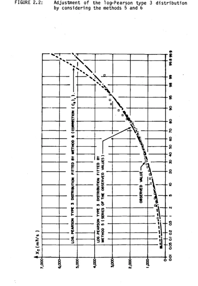
(2.33 ) 1 1

2.2.6 The Log-Pearson Type 3 Distribution

A. Characterization of the distribution

The log-Pearson type 3 distribution is deduced from the Pear-son type 3 distribution by a logarithmic transformation:

If Y

=

Ln X follows a Pearson type 3 distribution, X follows a log-Pearson type 3 distribution. It can be shown (Bobée, 1975) that the density function of the variate X is:

sion:

10.1

am f (x)

= _ _ _

e_ [a (Ln x - m)

i-

1 a > 0 a. < 0 r (À) 1

+0.

X m e ~ x m

o

~ x ~ e (2.34 )

The non-central moment of order r i s given by the

expres-III

=

r

The log-Pearson type 3 distribution includes the log-normal distribution in the limiting case where À tends towards infinity.

B. fvlethod of moments

The hydrology committee of the Water Resources Council in the United States recommends the use of the method of moments to logarithmically transformed samples (y

=

Ln x) of observed values (Benson, 1968). This method may be described as follows: from the observed sample Xl, ••• , xN' the transformed sample YI' ••• , Yn is obtained such that Yi

=

Ln xi (one may also

consid-er a base -10 logarithmic transformation for instance). The mean (ml) , unbiased variance (S2) and corrected coefficient of

skew-IY y '"

ness (C) are then cal cul ated and the event YT i s deduced from s Y

Y

=

(ml) + K s

T l Y T Y (2.35)

where K is the Pearson type 3 frequency factor corresponding to a

T

return period T and to a skewness coefficient (C) (equation s Y

,.. """

2.29). Since we have YT

=

Ln x_T we can deduce:

from which we obtain asymptotically: 1 "

= -

Var (X T) "2 X T (2.37)

Note that when the base -10 logarithmic transformation is used, we have asymptotically:

with

1

A

=

Logl 0 e

=

=

0.434

The method of moments based on the logarithmic transformation of the observed sampl e, cornes to give the same wei ght to the logarithms of the observed values. Each observed value, however, no longer has the same weight. Moreover, it is the moments of the sampl e of 1 ogari thms whi ch are preserved and not the moments of the sample of observed values. Consequently this method tends to reduce the rel ative importance of the 1 arger el ements of the sample.

C. The method of moments appl i ed to the sampl e of observed values

This method (Bobée, 1975) conserves the moments of the sample of observed values and gives the same weight to each observation.

We consider the three first non-central moments of the sample, ml, ml and ml which are estimations of the moments ~I, ~I

l 2 3 l 2

and ~I of the population. Equating these first three sample 3

moments to the corresponding popul ation moments, the following system of equations is obtained:

Ln [(1 - 1/a}3 1 (1 - 3/a)] Ln m_{3 -} 3 Ln ml

---=---

_{Ln [(1 - lia)}

2 1 (1 - 21 a)] Ln ml - 2 Ln ml

Ln m2 - 2 Ln ml À

= _ _ _ _ _ _ _ _ _ _

_

Ln [(1 _ 1/a)2 / (1 - 2/a)J m

=

Ln ml + À Ln (1 - 1/ a) l (2.38 )

The solution of the first of these equations for a may be obtained with the help of available tables (Bobée, 1975) or by approximations given by Bobée and Boucher (1981 a). Ki te (1978) al so gives approximati on formul as for determi ni ng a from thi s equation.

Knowi ng a we may cal cul ate À and then m usi ng the l ast two

equations of (2.38). We may hence estimate the moments (~~)p and

(~) along with the coefficient of skewness yp of the

corre-2 p

sponding Pearson type 3 distribution. YT

=

Ln x

T is then calcu-YT

lated using relationship (2.2), and finally x_T

=

e is deduced. ,..

The calcul ation of Var (X

T) for this method of estimation is

A

indicated in (Bobée and Boucher, 1981 b) but the form of Var (X T) (and therefore of 0T) is not explicite

From a, À and m (or from the non-central moments), the mean,

vari ance and coeffi ci ent of skewness of the popul ati on may be determined.

Hoshi and Burges (1981) describe a method for estimating X

T

A

and Var {X

T} for the log-Pearson type 3 distribution based on estimates of the mean, coefficient of variation and skew coefficient obtained from the observed (untransformed) sampl e. This method leads in practice to the same results as the method of Bobée {1975} that we have just described.

D. Method of maximum likelihood

The equations of maximum likelihood obtained for the variate X, which follows a log-Pearson type 3 law, correspond to the equa-tions of maximum 1 ikel ihood for the Pearson type 3 distribution with Y = Ln X.

In practice, i t suffi ces to 1 ogari thmi cally transform the originally observed sample (Xl ••• xN), to obtain the sample

(YI ••• YN) with Yi

=

Ln xi·

The appl ication of the method of maximum 1 ikel ihood to the sampl e Y., whi ch i s supposed to be drawn from a Pearson type 3

l

".. ".. A.

",..

One can thus deduce the event YT of return period T and then .... _YT

compute x_T

=

e • It is equally possible to determine the asymp-totic variance Var

(Y

T) and to deduce var

(X

T) which is equal to

"... A.

(X

T}2 var (YT) (to a first order asymptotic approximation).

However, as in the case of the method of maximum likelihood appl ied to the Pearson type 3 distribution, properties of the method are asymptotically optimal and theoretically the method is only viable for large samples (Bobée, 1979). The restrictions and the particularities of the method of maximum likelihood, for the log-Pearson type 3 distribution, are the same as those described in section (2.2.5 C) for the Pearson type 3 distribu-tion.

2.2.7. Goodness-of-fit Tests and Comparison of Frequency Distributions

Tests of goodness-of-fit, or test of ad justm en t, are a means of verifying whether a probability density function f (x) repre-sents the observations (or the sample). Among the most commonly used tests of goodness-of-fit are the chi-square test and the Kolmogorov-Smirnov test. Unfortunately, however, with the usual sample sizes of flood data none of the existing tests of adjustment are powerful enough to di scrimi nate between di fferent probability distributions.

A. Chi-square test

The statistic x2 _{is a measure of the deviation between the} observed number of events (Di) and the theoretical number of events (e.). The deviation

1

k (Qi - e.) 1 2 k Of 1

x

2 ₌

_l

₌

_l

--

_{N (2.39 )}

i=1 e. i=1 e.

1 1

follows approximately a chi-square distribution (x2 ) with y

degrees of freedom, where y = k - P - 1, in which:

k: number of class intervals;

p: number of parameters defining the probability density function f* (x) that are estimated beforehand from the sample, to make f* (x) a completely specified function.

In practi ce therefore, to apply the x2 _{test, the N i} ndepen-dent observations of the sample are grouped into k classes and the number of observations O.in each class, is determined. We

1

k

therefore have

l

Di = N. i=1