Prof. S. K. Burns Prof. P. R. Grayt Prof. R. W. Henry$ Prof. P. G. Katona Prof. N. P. Moray** Prof. W. T. Peakeft Prof. W. A. Rosenblith Prof. W. M. Siebert Prof. T. F. Weisstt Prof. M. L. Wiederhold J. E. Berliner L. D. Braida H. S. Colburn P. Demko, Jr. J. J. Guinan, Jr.
Academic and Research Staff Dr. J. S. Barlowjj Dr. G. O. Barnett*** Dr. A. Borbelyttf Dr. A. W. B. Cunninghamt$$ N. I. Durlach Dr. R. P. Erickson**** Dr. O. Franzenttttf Dr. G. Gambardella Dr. R. D. Hall
Graduate Students
R. M. Hershkowitz
H. S. Hsiao
E. G. Merrill
E. C. Moxon
M. J. Nahvi
R. E. Olsen
Dr. G. Hellekant$$f$ Dr. N. Y. S. Kiangtf Dr. M. Nomoto**** Dr. K. Offenlochttttt Dr. R. Rojas-Corona Dr. G. F. Songster R. M. Brownt A. H. Crist"t W. F. Kelley D. P. Langbeint R. E. Peterson S. E. Portny D. J-M. Poussart I. H. Thomae J. J. WawzonekThis work was supported principally by the National Institutes of Health (Grant
1 P01 GM-14940-01), and in part by the Joint Services Electronics Program under
Con-tract DA 28-043-AMC-02536(E).
Leave of absence, now at General Atronics Corporation, Philadelphia, Pennsylvania.
lVisitingAssociate Professor from the Department of Physics, Union College,
Schenectady, New York.
Visiting Associate Professor from the Department of Psychology, University of
Sheffield, Sheffield, England.
"Also
at the Eaton-Peabody Laboratory, Massachusetts Eye and Ear Infirmary,
Boston, Massachusetts.
"Research Affiliate in Communication Sciences from the Neurophysiological
Labo-ratory of the Neurology Service of the Massachusetts General Hospital,
Boston,
Massachusetts.
Associate in Medicine, Department of Medicine, Harvard Medical School, and
Director, Laboratory of Computor Science, Massachusetts General Hospital.
Postdoctoral Fellow from the Brain Research Institute, University of Zurich,
Zurich, Switzerland.
"Research
Associate, Department of Pathology, Peter Bent Brigham Hospital,
Boston, Massachusetts.
Visiting Scientist from the Department of Psychology, Duke University, Durham,
North Carolina.
""Postdoctoral
Fellow from the Speech Transmission Laboratory, The Royal
Institute of Technology, Stockholm, Sweden.
Postdoctoral Fellow from the Department of Physiology, Kungl. Veterinarskolan,
Stockholm, Sweden.
Public Health Service International Postdoctoral Research Fellow, from the
Department of Physiology, Tokyo Medical and Dental University, Tokyo, Japan.
"m
Postdoctoral Fellow from the Max Planck Institute for Brain Research,
Frankfort, Germany.
A. PRELIMINARY WORK ON A NEW MODEL OF BINAURAL HEARING
This is a report of preliminary work on a model of binaural hearing in which the firing patterns on the auditory nerve are regarded as inputs to a central processor. The model is an extension of work done by W. M. Siebertl '
2 on monaural phenomena. The representation of the firing patterns is based upon data taken from the cat's auditory nerve by N. Y. S. Kiang and his collaborators.3 The major assumptions in the prelim-inary version of the model are: (i) the activity in the nerves is characterized by the firing times of the fibers, and the inputs to the central processor are sample functions from random-point processes l '
2 in which the processes corresponding to the two ears are independent; (ii) the central processor is ideal, subject to the limitation that it only makes use of the times between firings, that is, it has no absolute time reference. By comparing the predictions of this version with psychoacoustic data, we can separate the limitations on performance imposed by the peripheral transformation from the limita-tions imposed by the central processor. These results can then be used to guide the development of a more realistic model of the processor.
We begin by presenting some general predictions that are independent of the random process selected to describe the firing patterns. We then choose a particular process and derive further predictions based on this process. Finally, we compare these pre-dictions with available data. The prepre-dictions are made for situations in which the listener is required to discriminate interaural time delay or interaural amplitude ratio for tone bursts in a two-alternative-forced-choice experiment. We consider the just-noticeable difference (JND) in interaural time and interaural amplitude as a function of the ampli-tudes in the two ears, the interaural time delay, the frequency, and the duration of the tone. We assume that the task of the subject is to correctly identify the order of pre-sentation of two binaural stimuli (a and b) that are identical except for incremental dif-ferences in interaural time or interaural amplitude, and that the JND is defined as the difference for which the probability of a correct response is 0. 75. It can be shown that, under reasonable assumptions, the JND is equal to a constant factor times the variance of the minimum-variance estimate of the difference.
For interaural time,
stimulus a: s (t) = A1 cos w - T - s2(t) = A2 cos w +
)
stimulus b: sl (t) = A cos c - T + s2(t) = A2 cos W
stimulus a:
stimulus b:
sl(t) = A1 1 + cos (t-T)s (t) = A
1 (cos W(t-7)
s
2(t) = A2 -s2(t) = A2(i
+The following notation is used throughout this report:
sj(t)
=
pressure signal to ear j (j=l, 2)
A. = reference amplitude of signal to ear j
6 = incremental difference in interaural amplitude ratio to be detected T = reference interaural time difference
A = incremental difference in interaural time to be detected
t. = received data vector for ear j = firing times of all fibers of nerve -J in ear j t = (t t ) p(t /A, y)
-j
6o(A
1, A2, T) = Ao(A1, A2, T) =probability density function for t. in response to the stimulus s.(t)= A cos (t-y)
value of 6 such that the probability of being correct is 0. 75 when amplitudes are Al and A2 and the interaural delay is T
value of A such that the probability of being correct is 0. 75 when amplitudes are Al and A and the interaural delay is T
a = estimate of a (where
a
is any parameter).
We note here that, because of the assumption of ideal processing, 6o(A
1, A
2,
T)and
Ao(A
1, A2, T) are independent of T. This is obvious when one considers that the idealprocessing has perfect memory of interfiring intervals.
This is an artificial
assump-tion and perfect memory will not be included in future versions of the model. In keeping
with these statements, we shall restrict our attention to the case
T =
0, and
Twill be
suppressed in our notation, since the predictions of the preliminary version are
inde-pendent of T.In order to ensure that the central processor only makes use of the times between
firings, we introduce an unknown time delay 0 which is the same for both ears and
dif-ferent for each burst. (This has the effect of allowing the subjects to detect only
inter-aural differences in time delay and, therefore, the interinter-aural delays
Tand A can be
split up arbitrarily between the ears.) The reference stimuli (A= 0= 6) during a
icos wtparticular burst can now be written
sl (t) = Al cos W(t-0) s2(t) = Az cos w(t-@).
In the following discussion, we shall use Crambr's bound4 on the variance of an esti-mate ^, extended to the case of an unknown parameter. 5 If Var ['] is the variance of a,
t is a received data vector, and f(t/a, 0) is the conditional probability of
1,
given a and0, the bound is
Ea ln f(t/a, 0) E
I\---Var
[a]
L\
ao
8 nf(/a, 0 8 n f(t/a,O ) 2 z8 n f(t/a, 0) a
In f(t/a,
0)
E 80 80
8a 80
Note that when
F8
ln f(t/a, 0) a ln f(t/a, 0)E 8a 8 = 0, (1)
the bound can be written
a,
1
Var
[]
1a ln f(t/a, 0)
E
aa
In all cases, there exists an estimate whose variance achieves the bound, at least asymptotically, and, therefore, we shall use the bound with equality. For simplicity, we assume that Eq. 1 is satisfied by p(jt/A, y) and thus, that lack of knowledge of y does not affect the estimate of A. That random processes exist which describe the data rea-sonably well and satisfy Eq. 1 is demonstrated by the example discussed later in this report.
For convenience, we introduce the notation
1
o((A) = a In p(t j/A, y) 2
aA
I
2
2
This notation is reasonable, since cr (A) and a (A) are positive and are independent of y if edge effects are ignored.
is P(t 1/A 1 , +) P(t/A 2 ,
O-)
, where we have assumed for simplicity that the ears are statistically identical, as well as statistically independent. We can now prove thatVar[] = -2(A l) + a (A2) = 4A2(A1,A 2)
and, therefore, that the interaural time JND on the midline is
1
A
(A, A) = - -(A), (2)o
,
-A
and the JND' s off the midline are related to those on the midline by
A
2o(A
1, A2) =
(A
2 (A1,A 1)
+ 2(A
2, AZ)).
(3)
Proceeding similarly for the interaural amplitude case and using the assumption that Eq. 1 is satisfied, we obtain
4 2
Var[] 1 1 =46 o(Al A 2 )
2 2
Y
(Al
)a-(A)
It follows directly that the interaural amplitude JND on the midline is 1
S0(A, A)= a-(A), (4)
and the JND's off the midline are related to those on the midline by
2 (A A( 1 1 5)
6
2(A
1, A
2)
=+
0 16 o2(A1' Al) 62(A2 , A Z )
If we assume that 6 (0, 0) = o, then
2 2
2(A, 0) 26 (A, A) (A); (6)
that is, the monaural amplitude JND is equal to NTZ times the interaural amplitude JND on the midline.
Equations 2-6 summarize the general predictions; in the sequel we shall assume a particular form for p(t /A, y), which is based on the neurophysiological data of N. Y. S.
3j
Kiang.3 We assume that the individual fibers are independent and that the firing times for the ith fiber (1< i-< M) can be modeled as a sample function of a nonhomogeneous
6
Poisson process, with intensity function ri.(A, t). (For a discussion of the applicability
1
1, 2
of the Poisson model to auditory nerve firing patterns, see Siebert .) With these assumptions and notation, we obtain
M2
-1
Z
C
T
1(
r.(A, u) l (A) 0 ri(A, u) u d (7 and(M
T
A
2r(A, u) 2
-0-(A) =d)
0 r (A, u)
aA
du
.(8(8)
=
Based again upon Kiang's data,3
a reasonable choice for low-frequency tones (and one for which Eq. 1 is satisfied) is
ri(A, t) = ai exp[gi(A, w) cos wt]. (9)
Here ai represents the spontaneous activity of the fiber, and gi(A, w) is a function that flattens to a constant at large intensities and includes the frequency selectivity of the fiber. For higher frequencies ri(A, t) becomes progressively less time-dependent until, at frequencies greater than ~5 kHz, the time dependence is not present. We shall
consider only the low-frequency case.
Using Eqs. 7, 8, and 9, we obtain approximately M
21A T 2 aig (A, w) Fo[gi(A, w)] (10)
i=1
M
2
2d
1 2 (agi(A, w) d o(x)
2 =TA ai Ak , (11)
(A)
i=1
dx
x=gi (A,w)
where
d2I (x)
Fo(x) = Io(x)
20 0 dx
and Io (x) is the modified Bessel function of the first kind of zero order. As indicated in Eq. 6, o-(A) is equal to the monaural amplitude JND studied by Siebert. 1
He has derived and evaluated (approximately) a summation equivalent to Eq. 11. We refer to his paper for a justification of the following statements:
(i) For A near threshold, 5 (A, A) decreases monotonically with A, perhaps as rapidly as A- 2 .
(ii) For larger values of A, 6 (A, A) is approximately constant. (iii) 62(A, A) is largely independent of frequency.
Equation 10 can be evaluated by methods essentially equivalent to those used by Siebert for Eq. 11. At low frequencies, the summation in (10) is approximately independent of frequency. Increasing A increases the number of fibers whose firings are synchronized with the variation of the stimulus, and more fibers are available from which information about the time structure can be obtained. At low intensities the increase is rapid; at higher intensities the number is dependent on the spread of stimulus-locked activity to fibers that are most sensitive to neighboring frequencies.
The resulting predictions for A (A, A) and 6 (A, A) are the following.
O O
For values of A well above threshold, K A (A, A) = (12) o TwZ(K + In A) K 6 2(A,A) = ' (13) o T
where K , KI' and K2 are constants.
For values of A near threshold, A0(A, A) and 6 (A, A) increase more rapidly with decreasing A.
We now compare the predictions expressed by Eqs. 2-6, which are independent of the random process chosen to model the firing patterns, with psychoacoustic data taken by R. M. Hershkowitz7 and reported in Section XIII-B. The experiment described there satisfies the assumptions implicit in our formulation. (Note that the incremental ampli-tude JND's in Sec. XIII-B are given in decibels, while, in the present formulation, 60 is a fraction.) Generally speaking, the interaural amplitude JND's were found to be independent of interaural time difference and to be consistent with Eq. 5. Since the magnitudes of the predicted and observed changes were of the order of the variability of the data, however, this is not a sensitive test of the model. In the case of interaural time JND's, the results were strongly dependent on interaural time delay T, and for values of T > 600 4sec, conflicting cues and other little understood effects made it impossible to reliably measure JND's. It is not surprising that these results are not predicted by the model, since 1) we have assumed perfect memory of all interfiring times, and 2) we have not taken into account the ambiguities in the region near the antiphasic point of a tone. (This was 1000 sec in the experiment above.) A comparison of the interaural time JND's on and off the midline with the relation predicted by Eq. 3 also revealed inconsistencies. As ear 2 was attenuated relative to ear 1, the JND increased much more rapidly than predicted. In fact, with ear 1 at 55 dB SPL and ear 2 at 25 dB SPL, the time JND was larger than when the ears were equal in ampli-tude at any level measured (measurements included values from 15 dB SPL to 80 dB SPL). This illustrates a significant and unexpected failure of the model which
should be useful in future work.
Experimental results will now be compared with the predictions of the model when
the Poisson process with the intensity function in Eq. 9 is chosen to describe the firing
patterns.
First, using Eq. 10 with reasonable values for a
i ,gi(A,
w),
and Fo(gi(A,
w)),
the interaural time JND for 500 Hz and 55 dB SPL is predicted to be roughly 1 4sec, as
compared with values of approximately 10 [isec in most empirical determinations.
7,
8This discrepancy could be due to the approximations and guesses made in the evaluation
of Eq. 10.
It seems more likely, however, that the discrepancy results from the ideal
processing assumption, which excludes significant time uncertainty in the higher centers.
Second, for values of A near threshold, the data and the predictions show an increase in
JND's with decreasing A.
(This, of course, would be predicted by almost any model.)
Finally, for higher values of A, the predictions expressed in Eq. 12 are generally
con-sistent with the data. The frequency dependence of A (A, A) corresponds well with the
8
odata of Klumpp and Eady for frequencies below 500-1000 Hz. At higher frequencies,
the interaural time JND increases and is essentially infinite at 1500 Hz. An increase at
higher frequencies is expected, because of the loss of time dependence of ri(A, t);
how-ever, this is not yet quantified in the model and may not be a sufficient explanation. The
dependence on duration has not been tested. The amplitude dependence in Eq. 12
pre-dicts that, when A increases from 40 dB to 80 dB, the time JND decreases to a value
between the value at 40 dB and 1/\FZT
times the value at 40 dB.
The data from
Hershkowitz
7in Sec. XIII-B indicate that
A
(A, A) [To(P
)in Hershkowitz' notation] is
constant or decreases slightly in this range, which is consistent with the model. Because
of the magnitudes of the effects, however, this is not a sensitive test of the model. For
a discussion of Eq. 13, we refer to Siebert.1 2
The results of comparing the predictions of the preliminary version of the model
with empirical data can be summarized as follows: in the case of interaural time, the
model predicts performance that is better than the data; and in the case of interaural
amplitude, the predictions are consistent with the data, although the effects are not
large enough to provide a sensitive test of the model. Steps will now be taken to put
con-straints on the operations available to the central processor, in the hope of obtaining a
model that better describes the behavioral data and of gaining insight into the processing
that takes place in the physical system.
H. S. Colburn
References
i.
W. M. Siebert, "Some Implications of the Stochastic Behavior of Primary Auditory
Neurons," Kybernetik
2
(5), 206-215 (June 1965).
2.
W. M. Siebert,
"Stimulus Transformations in the Peripheral Auditory System,"
Recognizing Patterns, P. Kolers and M. Eden (eds.) (The M. I. T. Press, Cambridge,
Mass. (1967).
3. N. Y. S. Kiang, Discharge Patterns of Single Fibers in the Cat's Auditory Nerve (The M. I. T. Press, Cambridge, Mass., 1965).
4. H. Cram6r, Mathematical Methods of Statistics (Princeton University Press, Princeton, N.J., 1946).
5. H. L. Van Trees, Detection, Estimation, and Modulation Theory (John Wiley and Sons, Inc., New York, 1967).
6. E. Parzen, Stochastic Processes (Holden-Day, San Francisco, 1962).
7. R. M. Hershkowitz, "Auditory Discrimination of Time and Intensity off the Midline," S.M. Thesis, Department of Electrical Engineering, M. I. T., September 1967. 8. R. G. Klumpp and H. R. Eady, "Some Measurements of Interaural Time Difference
Thresholds," J. Acoust. Soc. Am. 28, 859-860 (1956).
B. DISCRIMINATION OF INTERAURAL TIME AND INTENSITY OFF THE MIDLINE
In most previous work on interaural just-noticeable differences (JND's) in time and amplitude, the JND's have been measured only on the midline. 1 Moreover, the time JND's and amplitude JND's have usually been measured in separate experiments (with differ-ent methods, subjects, and equipmdiffer-ent), so that it is difficult to evaluate predictions on the relations of the two types of JND's.
In our research, we have performed a preliminary experiment on time and ampli-tude JND's both on and off the midline with a common experimental configuration and a common set of subjects. Specifically, we have made preliminary estimates of the fol-lowing 6 functions: (i) interaural amplitude JND a as a function of interaural amplitude difference a; (ii) interaural time JND T as a function of interaural time difference T; (iii) interaural amplitude JND a as a function of interaural time difference
7;
(iv) inter-aural time JND T as a function of interaural amplitude difference a; (v) interauralo
amplitude JND a on the midline as a function of signal level P; and (vi) interaural time JND r on the midline as a function of signal level P.
The method used to obtain the JND's was two-alternative-forced-choice-plus-feedback. The signal was a 500-Hz tone burst of 300-msec duration. The rise and decay times were 50 msec, the interstimulus interval was 300 msec, and the subject had 1. 6 sec in which to respond. Except when the signal level P was the independent variable (functions 5 and 6), the reference level in the left ear was maintained at
55 dB SPL. The incremental difference in amplitude for obtaining the JND in interaural amplitude was obtained by raising the signal in one ear and lowering the other, and the JND a refers to the total difference. When an interaural amplitude difference a of
non-unity was required as a reference, however, it was achieved by decreasing the amplitude in the right ear below 55 dB, with the amplitude in the left being held constant at 55 dB. Thus, when a = 55 dB, the presentation was essentially monaural. In all cases, the
JND was defined as the increment (in time or amplitude) for which the subject's responses were 75% correct. Two experienced subjects, LW and ND, were used throughout the experiment, and each of the 6 functions was measured at least twice on
each subject. Because of the large number of JND's to be measured, it was impossible (within the given time constraints) to obtain complete psychometric functions in esti-mating the JND. Instead, a crude, informal, homing technique was used. In this tech-nique, a few brief runs of 30 trials or less were presented first in order to locate the general region of the JND. Having located this region, 2-3 runs of 100 trials were then made to estimate the JND.
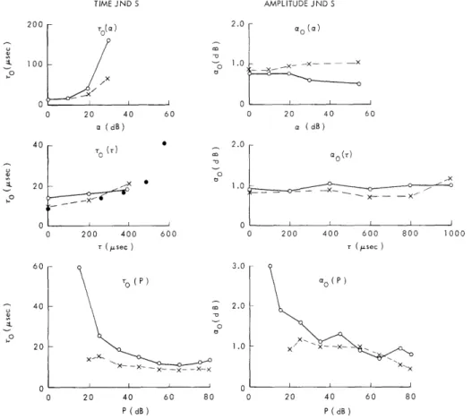
The results of the experiment are shown in Fig. XIII-1. For the on-the-midline JND's, these results can be compared with those of Mills2 (amplitude JND) and those of Klumpp and Eady3 and Zwislocki and Feldman4 (time JND). Our average results at P = 55 dB SPL are roughly ao = 0. 9 dB and
To
= 11 [sec, and the average increase inTIME JND S ro(a)0 AMPLITUDE JND S ao (a) 1.0J __,_-x 0 20 40 a (dB) 0 200 400 r ($sec ) ro (P) 40 [ 0 20 40 60 a (dB) 2.0 1.0 0 1 1 0 200 400 600 800 10( r (Lsec ) 3.0 a ( P ) 00 2.0 1.0 x- x ---0 20 40 P (dB) 60 80 X', X I I I J 0 20 40 P(dB) 60 80
Fig. XIHI-1.
Just-noticeable differences in interaural time and aural amplitude for a 500-Hz tone as functions of inter-aural time T, interaural amplitude a, and power level P. O: Subject ND; X = Subject LW; e: translation of minimum audible-angle data obtained by Mills.5T
as P is decreased from 80 dB to 30 dB is ~7
psec.
The comparable previous results
o
are approximately ao
=
0. 7 dB, To
=
18 4sec, and an increase in To of ~7 -sec. Assuming
that changes in the azimuth of a tone source in a free-field environment are detected by
observing variations in interaural time (a reasonable assumption at 500 Hz), one can
translate the data of Mills on the minimum audible angle
5into data that can be compared
with our data on
T (T).The results of this translation (under the assumption that the
head is a sphere of 17-cm diameter) are shown along with our data on
To(T).
The fact
that our data on a (T) are essentially independent of
Tis inconsistent with the result of
6Mo
Mills
6which indicates that at 500 Hz the amplitude JND for antiphasic tones
(corre-sponding to
T = 1000p
sec) is smaller than that for homophasic tones
(T =0).
By taking the ratio To/ao
,
our results can also be compared with those of Moushegian
and Jeffress
on time-intensity trading.
In their experiment, the listener was
pre-sented with a 500-Hz 75-dB SPL tone with interaural delays in the range 0-360 [Isec and
interaural amplitude ratios a in the range -9-+9 dB, and he was required to set the
interaural time delay T' of a noise signal to match the lateral position of the tone.
The
results for the 3 subjects tested in their experiment were roughly the following.
For
each subject, and each value of
T,
the dependence of
T'on a was approximately linear
(a measured in dB) with T' = T at a = 0 dB. For subject1,
the slope of T'(a) was2. 5
psec/dB
for all
T.For subject 2, the slope was 18 isec/dB at
T =0 and increased
monotonically to approximately 30
psec/dB
at
T=
360 tsec.
For subject 3, the slope
was 27 sec/dB at T = 0 and increased to ~40[sec/dB
at T = 360-sec.
Assume now that the effects of interaural time and interaural amplitude can be
described purely in terms of a common, unidimensional, lateralization sensation (that
is, that time and amplitude are completely tradeable) and the discrimination cue in our
experiment for both the time JND and amplitude JND is derived solely from this
sensa-tion. Under this assumption (which, at best, can only be approximately valid in a region
around the midline), we would expect our results on
T0/a
0to be approximately equal to
the ratios just cited. According to our data on
To(P)and ao (P), above approximately
30 dB SPL, the midline ratio To/ao lies in the range 9-21 ksec/dB (LW) and
11-16 4sec/dB (ND).
The corresponding values in the Moushegian-Jeffress experiment are
those for which
T=
0 and are 2. 5, 18, and 27 i sec/dB. According to our results on
TO(T) and ao (), as T increases from 0 to 400
Lsec,
the ratio T (T)/a (T) increasesfrom ~12 to 24
sec/dB (LW) and 17 to 18 Jsec/dB (ND).
The corresponding results
from the trading experiment are 2. 5 to 2.5
psec/dB,
18 to 30 ksec/dB, and 27 to
40 ~sec/dB.
In general, the difference between the results obtained in the two
experi-ments is no greater than the difference between the results obtained by different
sub-jects in either of the two experiments alone.
In considering our data on
TO(T),
it is important to note that the graph terminates at
T=
400 isec only because we were unable to obtain reliable JND's for values
of T > 600 Lsec. At these larger values, the subjects found substantial changes in the
dis-crimination cues and tended to become very confused. In particular, the subjects
claimed that cues tended to reverse (in the sense that the stimulus that was leading in
the left ear produced an image to the right of the stimulus that was leading in the right
ear).
In order to document this confusion, an additional short experiment was carried
out. In this case, the incremental time disparity AT was held constant at AT
=
100 Jtsec,
and the value of the reference delay
Twas varied from 500
sec to 1000 Fsec. In
addi-tion to ND, who participated in the main experiment, two addiaddi-tional subjects, RH and
SC, were used. In order to keep track of cue reversals, the subjects were instructed
to maintain a constant response code and reminded that getting all the answers wrong
was just as good as getting them all right. The results of this experiment (in which
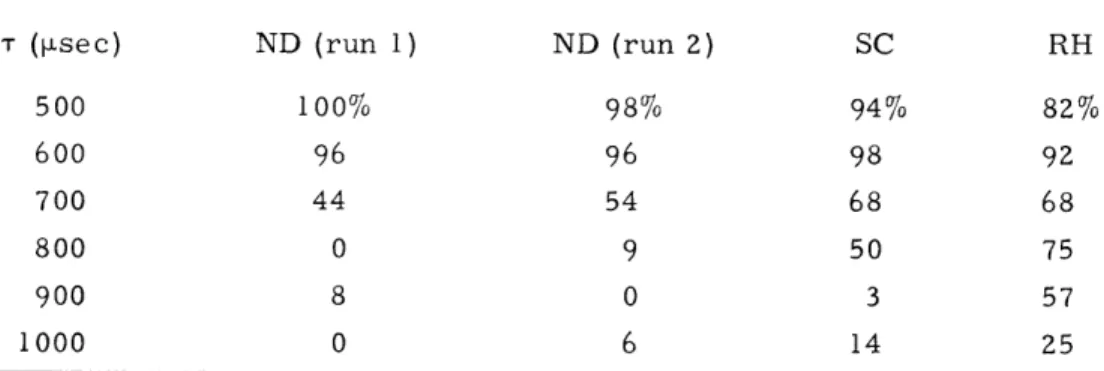
each run consisted of only 50 trials) are shown in Table XIII-1.
Note how the cues
Table XIII-1. Per cent correct as a function of 7 for AT = 100
[isec.
T
( isec)
ND (run 1)
ND (run 2)
SC
RH
500
100%
98%
94%
82%
600
96
96
98
92
700
44
54
68
68
800
0
9
50
75
900
8
0
3
57
1000
0
6
14
25
tended to reverse and that near the point of reversal, the discrimination performance
becomes very poor. Unfortunately, we did not have sufficient time to fully explore this
phenomenon.
It is our conjecture, however, that it is related to the "headwidth
limita-tion" discussed in connection with binaural unmasking
8and to the lateralization
ambi-guity associated with the antiphasic point at
T=
1000
psec.
It is interesting to note in
this connection that Mills reported a similar phenomenon at large angles in his
mini-mum audible angle experiment.
5The primary purpose of our experiment was to provide data to help guide the
devel-opment of Colburn's auditory-nerve model of binaural processing (see Sec. XIII-A).
Based on the perfect-memory assumption (known to be inadequate), the model predicts
that T (-T) and a (T) should be independent of T. This prediction is satisfied for a (T), but not for T (T). With regard toa
(a), the model predicts a small increase as weleave the midline (e. g., a maximum increase of 0. 3 dB when the midline JND is in
the range 0. 8-0. 9 dB). This prediction is consistent with the LW data, but not with the
ND data. The data on T (P) and a (P) show that at very low levels,
Tand a
increase
with a decrease in P, as Colburn's model (or any other model) predicts. At
moderate-to-high levels, the data on T (P) are relatively constant. According to the model, as
P increases from 40 to 80 dB, T (P) must decrease by a multiplicative factor q in the range 0. 7 -< q < 1. 0. For a (P), the data show that a decreases slightly at moderate-to-high levels as P is increased, whereas the model predicts that a should be constant in this region. Aside from the case of T (T), the most serious discrepancy occurs with To(a). Making use of the data on T (P) and Colburn's equation relating T (P) to T (a),
we find that the prediction for T (a) seriously underestimates the growth of T with a.
For example, at a = 30 dB, the predictions for ND and LW are 20 and 12 tsec, respec-tively (as compared with the empirical values of 160 and 41 sec).
A second purpose of the experiment was to test the prediction of Durlach's equal-ization and cancellation (EC) model relating time JND's on the midline to amplitude JND's on the midline.9 According to this model, one should have a (dB)/T 0
8. 7 (2Trf o/Nf), where fo is the frequency of the tone, and k is a frequency-dependent parameter of the model that includes the error variances associated with the "jitter" in the EC process. Assuming that k = 1. 185 at 500 Hz (a value often used by Durlach in binaural unmasking applications and in the initial JND applications), we obtain ao(dB)/To(iLsec) = 0. 025. According to our results, however, the ratio is 0. 08 (LW) and 0. 07 (ND). Moreover, since the model requires that k >, 1, there is no value of k for which the model predicts a ratio greater than 0. 028.
Further details on this research are available in the author's Master's thesis.10 R. M. Hershkowitz
References
1. The word "midline" refers to the position of the signal image in perceptual space. 2. A. W. Mills, "Lateralization of High-Frequency Tones," J. Acoust. Soc. Am. 32,
132-134 (1960).
3. R. G. Klumpp and H. R. Eady, "Some Measurements of Interaural Time Difference Thresholds," J. Acoust. Soc. Am. 28, 859-860 (1956).
4. J. Zwislocki and R. S. Feldman, "Just Noticeable Differences in Dichotic Phase," J. Acoust. Soc. Am. 28, 860-864 (1956).
5. A. W. Mills, "On the Minimum Audible Angle," J. Acoust. Soc. Am. 30, 237-246
(1958).
6. A. W. Mills (personal communication, 1967).
7. G. Moushegian and L. A. Jeffress, "Role of Interaural Time and Intensity Dif-ferences in Lateralization of Low Frequency Tones," J. Acoust. Soc. Am. 31, 1441-1445 (1959).
8. L. R. Rabiner, C. L. Laurence, and N. I. Durlach, "Further Results on Binaural Unmasking and the EC Model," J. Acoust. Soc. Am. 40, 62-70 (1966).
9. N. I. Durlach, "On the Application of the EC Model to Interaural JND's," J. Acoust. Soc. Am. 40, 1392-1397 (1966).
10. R. M. Hershkowitz, "Auditory Discrimination of Interaural Time and Intensity off the Midline," S. M. Thesis, Department of Electrical Engineering, M. I. T., 1967.
C. EFFECT OF DURATION ON THE DISCRIMINATION OF PERIODICITY PITCH
It is well known that the frequency of a low-frequency tone is encoded in the neural firings of the auditory nerve in at least two ways: (i) by the set of fibers that respond to the stimulus (place encoding), and (ii) by the temporal patterns of the firings in a given fiber (time encoding). According to the model developed by W. M. Siebert, if the higher centers make optimum use of the place encoding but ignore the time encoding, the just-noticeable difference (JND) Af in frequency f should depend on the duration, T, of the stimulus according to the relation Af cc T . If, on the other hand, the higher centers make optimum use of the time encoding but ignore the place encoding, the relation should be of the form AfccT- 3/2
There are reasons for suspecting that the higher centers do not make optimum use of the time encoding. In order to provide a direct test, however, an experiment was performed to determine the JND in frequency as a function of duration for a stimulus in which the frequency discrimination would have to be based purely on time information. The stimulus selected was chopped, white, Gaussian noise, and the aspect of the stim-ulus to be discriminated was the chopping rate. As pointed out previously by Miller and Taylor,Z such a stimulus leads to a sensation of pitch (corresponding to the chopping rate), despite the fact that its spectrum is essentially the same as the unchopped noise, and it is believed to be very unlikely that the pitch arises from place encoding. According to the model, if the system makes optimum use of the timing information, the JND in chopping rate should vary with duration in the same manner as the JND for
tones under the assumption that the place information is ignored, that is,
AfccT3/Z
Our method was that of two-alternative-forced-choice-plus-feedback (a priori prob-abilities of 0. 5), and the subject's task on a given trial was to indicate which of the two signals in that trial had the higher chopping rate. The two base rates studied were 75 Hz and 300 Hz, the power level was 55 dB SPL, the duty cycle was 0. 5, and the range of durations considered was 40-600 msec. Each run at a given set of conditions consisted of 100 trials, and the JND was defined to be the increment in chopping rate for which the subject's responses were 75% correct. The JND was estimated by varying the increment from run-to-run, obtaining psychometric functions, and inter-polating. Four subjects were employed throughout the experiment.In attempting to obtain psychometric functions, several difficulties were encountered. First, the training problem seemed to be unusually difficult for this task, in the sense that it took an exceptionally long time for performance to stabilize. Second, the
psy-chometric functions were very often flat, that is, the %-correct responses varied very slowly with the increment in chopping rate. Thus, the results obtained for the JND's were less precise and less reliable than in many other experiments. In general, the experiment is regarded merely as a preliminary exploration, and it is clear that much
more work is required to obtain definitive results.
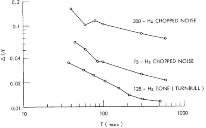
The JND's obtained for the two base frequencies and the various durations (aver-aged over subjects) are shown in Fig. XIII-2. The dip at 60 msec in the curve for
0.2 300 - Hz CHOPPED NOISE 0.1 < 0.04 - 75 - Hz CHOPPED NOISE 0.02 128 -Hz TONE ( TURNBULL ) 0.01 10 100 1000 T ( msec)
Fig. XIII-2. Weber fraction Af/f as a function of duration T.
300 Hz appeared in the data for each of the 4 subjects. The change in slope at the shorter durations for the 75-Hz case occurred for 3 of the 4 subjects. The slopes of these curves are approximately -0. 3 (300 Hz), -0. 3 (75 Hz, long durations), and -0. 9
(75 Hz, short durations). Unless one assumes that the slope continues to decrease as the duration is decreased below 60 msec, there is no indication in these results of
relation of the form JND c T- 3 / 2. Roughly speaking, the dependence of the JND on duration for the chopped noise appears to be approximately the same as the results obtained for tones (where there is place information, as well as time information). A comparison of the present results with those of Turnbull3 for a 128-Hz tone is included in Fig. XIII-2.
Further details about this study can be found in the author's Master's thesis.
S. E. Portny
References
1. W. M. Siebert, "Some Implications of the Stochastic Behavior of Primary Auditory Neurons," Kybernetik, Vol. 2, No. 5, pp. 206-215, 1965; also, "Limitations on Frequency Discrimination Imposed by the Statistical Character of Auditory Nerve Activity," (unpublished).
2. G. A. Miller and W. G. Taylor, "The Perception of Repeated Bursts of Noise," J. Acoust. Soc. Am. 20, 171-182 (1948).
3. W. W. Turnbull, "Pitch Discrimination as a Function of Tonal Duration," J. Exp. Psych. 34, 302-316 (1944).
4. S. E. Portny, "The Effect of Duration on the Discrimination of Periodicity Pitch,"
D.
SEQUENTIAL EFFECTS IN AUDITORY INTENSITY DISCRIMINATION
In psychophysical experiments, the response to a given stimulus depends not only
on the stimulus, but also upon the "state" of the subject at the moment the stimulus is
presented.
Previous research1 has shown that one important determinant of the
sub-ject's state is the sequence of previous events (previous stimuli, responses, and
experimenter-subject feedbacks) in the experimental run. Since this sequence changes
from trial to trial, the subject' s state must also be regarded as changing from trial to
trial. Although the dependence of state on the sequence of previous events is a generally
recognized fact, the structure of this dependence is not well understood. Furthermore, in
many of the models that are currently being used to interpret psychophysical data,
this dependence is ignored. A common procedure is to assume that the various trials
in a sequence are statistically identical and independent, and to interpret the
fluctua-tions in the subject's responses to a given stimulus in terms of some unspecified
"internal noise." In order to improve the quality of psychophysical research, it would
be useful to devise experimental paradigms in which the fluctuations in state caused by
variations in the sequence of previous events are minimized, or to understand this
phenomenon well enough to take proper account of it when analyzing the data.
In a preliminary experiment that has just been completed, we have studied the effect
of the just-previous trial on a subject's response in the context of a monaural,
two-alternative- forced- choice, intensity-discrimination task. In each trial, the stimulus
consisted of a pair of 350-msec, 400-Hz, tone bursts differing in intensity, and the
subject was required to judge which of the two bursts was the more intense. With I
denoting the mean intensity and AI the differential intensity (both in dB), the subject's
task was to distinguish between the high-low pair (I+ AI/2, I-AI/2) and the low-high
pair (I- AI/2, I+ AI/2). Each of these pairs was presented with an a priori probability
of one-half.
This experiment consisted of four parts, denoted cases 1, 2, 3, and 4. In cases 1
and 2 (the "fixed-level" cases), the value of I was held constant at 75 dB SPL. In
cases 3 and 4 (the "roving-level" cases), I varied randomly from trial to trial between
64 dB and 80 dB SPL (with a priori probabilities of one-half). In cases 1 and 3, the
subject received no feedback from the experimenter. In cases 2 and 4, the subject was
informed automatically after each trial whether or not his response was correct.
Four values of AI were tested in each case, and at least 2000 trials were presented
to each of 4 subjects at every value of AI. Thus, at least 32, 000 trials were presented
to each subject. Aside from the author (who served as Subject 3), none of the subjects
knew that the primary purpose of the experiment was to study sequential effects. It had
originally been intended to run some further tests in which the subjects were informed
of their sequential dependencies and instructed to eliminate them, but the available
time was not sufficient for this purpose.
The data from this experiment were recorded on punched paper tape and pro-cessed on the PDP-4 computer. The data processing consisted of computing two matrices: a zero-order matrix, and a first-order matrix. The zero-order matrix summarizes the results without regard for the previous trial and pre-sents information (for each value of Al) on the number of high-low trials, the number of low-high trials, the number of correct responses for each type of trial, the various relevant percentages, and the values of the parameters d' and
P'
of signal detection theory.2 The first-order matrix presents the same information as the zero-order matrix, but subdivided according to the events of the previous trial. Additional processing consisted of estimating the amount by which a given psychometric function would have been increased if the pre-vious trial had always been optimum (in the sense of leading to a maximum d' on the given trial) and if the subject's criterion had always been optimum (that is,p'
= 0). A brief description of some of the results of this analysis is given below.1. The effect of the just-previous trial depended strongly on the subject.
2. For those cases in which I was held constant, the difference between the opti-mum psychometric function (as described above) and the actual psychometric function was very small. For those cases in which I was varied, and for certain subjects, this difference was appreciable.
3. Subject 1 (whose over-all performance was exceptionally poor) showed a strong tendency to repeat consecutive responses in the no-feedback cases and a strong tendency to respond with the answer that was correct on the previous trial in the feedback cases.
4. Subjects 2, 3, and 4 showed a wide variety of small response dependencies. In addition to the dependency of p' on the previous trial, that is expected when feedback is introduced (that is, the adjustment of the criterion to improve performance), there were tendencies to (a) alternate responses when AI was small; (b) repeat responses when AI was large; and (c) respond oppositely to the previous presentation (interpreted as a microscopic adaptation effect, since it occurred when there was no feedback and increased with AI).
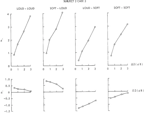
5. When the mean level I was varied from trial to trial, Subjects 1 and 2 showed a strong tendency to respond "low-high" when the given I was loud and "high-low" when the given I was soft. This effect (the usual macroscopic adaptation effect) was decreased, but not eliminated, by feedback. For Subject 2, most of this effect was attributable to the value of I on the previous trial. For Subject 1, the previous trial was not the dominant factor.
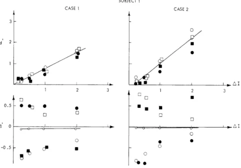
6. For most subjects and in most cases, the sensitivity d' was approximately a linear function of AlI. When the mean level I was fixed, this function was found to be
d 2[ 0.5 3 0 -0.5 Fig. XIII-3. E
Effect of previous trial on d' and
P'
for Subject 1 in cases 1 and 2. Previous trial code:O = previous trial high-low, answered correctly
0 = previous trial high-low, answered incorrectly O = previous trial low-high, answered correctly
0 = previous trial low-high, answered incorrectly.
Solid lines give d' and
P'
without regard to previous trial.SUBJECT 4 CASE 1 2 1 2 3 0.5 o * 030 -0.5 CASE 2 1 2 3 o o !oo • [•
Fig. XIII-4. Effect of previous trial on d' and
P'
for Subject 4 in cases 1 and 2. Previous-trial code as in Fig. XIII-3.independent of the stimulus on the previous trial, but to be steeper when the previous response was correct than when it was incorrect. This dependency occurred both with and without feedback, although it was stronger with feedback.
7. The slope of d'(AI) was increased by the introduction of feedback for Subjects 1 and 3, but not for Subjects 2 and 4 (whose performance without feedback was relatively good).
8. When the mean level I was varied from trial to trial, the slope of d'(AI) was appreciably smaller for the soft I than for the loud I. Also, the slope for the loud I in the variable-I cases was appreciably smaller than the slope for the fixed I cases. Some sample data from these experiments are shown in Figs. XIII-3, XIII-4, and XIII-5. LOUD - LOUD 4 3 d 2 0 0 1 2 3 1.0 0.5 (' 0 -0.5 -1.0 -1.5 SUBJECT 2 CASE 3
SOFT -LOUD LOUD -SOFT
'
/
0 1 2 3 0 1 2 3
SOFT- SOFT
0 1 2 3
AI ( d B)
Fig. XIII-5. Effect of mean signal level on d' and P' for Subject 2 in case 3. SOFT-LOUD means that the previous trial was
soft and the given trial was loud.
Further details on this work (as well as a comparison with earlier work) can be found in the author's Master's thesis.
References and Footnotes
1. See, for example, H. Helson, Adaptation Level Theory (Harper and Row, New York,
1964); I. Pollack, "Intensity Discrimination Thresholds under Several Psychophys-ical Procedures," J. Acoust. Soc. Am. 26, 1056-1059 (1954); I. Pollack, "Sound Level Discrimination and Variation of Reference Testing Conditions," J. Acoust. Soc. Am. 27, 474-480 (1955); I. Pollack, "Identification and Discrimination of Com-ponents of Elementary Auditory Displays," J. Acoust. Soc. Am. 28, 906-909 (1956); V. L. Senders and A. Sowards, "Analysis of Response Sequences in the Setting of a Psychophysical Experiment," Am. J. Psychol. 65, 358-374 (1952); V. L. Senders, "Further Analysis of Response-Sequences in the Setting of a Psychophysical Experi-ment," Am. J. Psychol. 66, 215-228 (1953); W. F. Day, "Serial Non-randomness in Auditory Differential Thresholds as a Function of Interstimulus Interval," Am. J. Psychol. 69, 387-394 (1956); W. J. McGill, "Serial Effects in Auditory Threshold Judgements," J. Exptl. Psychol. 53, 297-303 (1957); W. R. Garner, Uncertainty
and Structure as Psychological Concepts (John Wiley and Sons, Inc., New York, 1962), pp. 113-114; S. D. Speeth and M. V. Mathews, "Sequential Effects in the Signal-Detection Situation," J. Acoust. Soc. Am. 33, 1046-1054 (1961); R. C. Atkinson, E. C. Carterette, and R. H. Kinchla, "Sequential Phenomena in Psycho-physical Judgements: A Theoretical Analysis," IRE Trans., Vol. IT-8, pp. S155-S162, February 1962; R. C. Atkinson, "Variable Sensitivity Theory of Signal Detec-tion," Psychol. Rev. 70, 91-106 (1963); M. P. Friedman and E. C. Carterette,
"Detection of Markovian Sequences of Signals," J. Acoust. Soc. Am. 36, 2334-2339 (1964); E. C. Carterette, M. P. Friedman, and M. J. Wyman, "Feedback and Psychophysical Variables in Signal Detection," J. Acoust. Soc. Am. 39, 1051-1055
(1966).
2. In the version of signal detection theory that was used to analyze our data, it was assumed that the two density functions corresponding to the two stimuli I + A I/2 and I - A I/2 were Gaussian with means MH and ML and equal variance 2 , and that the listener responded "high-low" rather than "low-high" if and only if X1 - X2 P, where (X1, X2) is the pair of samples arising from the two-alternative-forced-choice presentation on the given trial, and
P
is the criterion. The parameters d' andP'
were then defined by the equations d' = 2(MH-ML)/a andP'
= P/u. To the extent that d' and p' depend on the events in the previous trial, the usual assumption that the probability densities and the criterion are constant from trial to trial is obvi-ously a false one.3. H. S. Hsiao, "Sequential Effects in Auditory Intensity Discrimination," S. M. Thesis, Department of Electrical Engineering, M. I. T. , September 1967.
E. SUBJECTIVE ESTIMATES OF UNCERTAINTY IN ABSOLUTE IDENTIFICATION
It has been shown in a variety of psychophysical tasks that the use of confidence ratings or second-choice paradigms can facilitate measurement without substantially decreasing performance level. The purpose of this research was to explore the extent to which similar benefits might be gained in a task of absolute identification.
The set of stimuli to be identified consisted of ten 1000-Hz, 500-msec tone bursts varying in level between 66 dB and 30 dB (SPL) in 4-dB steps. The stimuli were assigned numbers 1 through 10 in order-preserving fashion. The subject was not given
feedback, but before each run he was exposed to the whole set 3 times in decreasing order.
Two types of responses were employed. In the straight identification task (S), the subject responded with a single integer between 1 and 10 that represented his best guess as to the stimulus presented. In the weighting task (W), the subject was instructed to distribute numerical weightings over the set of stimuli according to the certainty with which he thought each stimulus was presented on the given trial. In each format, each
stimulus was presented 10 times in a given run, and the subject was given 10 runs with each format (S and W runs being alternated).
The data were processed to obtain three different confusion matrices. The S matrix was obtained from the S data in the usual fashion. The WP matrix was obtained from the W data by choosing the stimulus with the largest weighting as the response. The WA
matrix was obtained from the W data by normalizing the weightings on a given trial and averaging the weightings obtained for a given stimulus over different trials. It was found
that the information transfer, as well as the subject's biases, were roughly the same for all three matrices. It was also found that the widths of the distributions of weightings on a single trial in the W task was less than half of the widths determined from the WA and S matrices, and that the difference between the peak response and the average response in the W task was uncorrelated with the difference between the peak response and the correct response.
In general, we concluded that the additional burden in the W task of having to assign weightings did not degrade performance, but that the subject was unable to make use of the weightings to improve performance.
In future work, we intend to examine the extent to which the difference between the widths found on single trials in the W case and the widths found in the S and WA matrices (caused primarily by trial-to-trial variations in the peaks for the W case) can be ascribed to sequential effects.
Further details on this work can be found in the author's Bachelor's thesis.'
S. J. Bayer
References
1. S. J. Bayer, "A Psychophysical Study of Subjective Estimates of Uncertainty," S. B. Thesis, Department of Electrical Engineering, M. I. T. , June 1967.