Computational Design of Viscoelastic Gels with Tunable
Mechanical Energy Dissipation
by
Aarthy Kannan Adityan
Bachelor of Technology, Naval Architecture & Ocean Engineering Indian Institute of Technology Madras, 2011
Submitted to the Department of Mechanical Engineering in Partial Fulfillment of the Requirements for the Degree of
Master of Science in Mechanical Engineering
at the
MASSACHUSETTS INSTITUTE OF TECHNOLOGY
MASSACHUSETTS INSTITUVE OF TECHNOLOGY
AUG 15 2014
LiBRARIES
May 2014Massachu
etts
A C~-
zoi&IjqC 2014 Massachusetts Institute of Technology. All rights reserved
Signature redacted
Signature of Author... ... ...Departnfent of Mechanical Engineering
Signature redacted
MayI02014Certified by ... ...
Krystyn J. Van Vliet Associate Professor of Material ience and ineering and Biologi a Engineering
) /The s upervisor
Signature redacted
S ... Accei p te-d bkxy ... ... David M. Parks /01 rof4s in chaniedfngineeringSignature redacted
...
...
David E. Hardt Ralph E. and Eloise F. Cross Professor of Mechanical Engineering Chair, Committee on Graduate StudentsN
Computational Design of Viscoelastic
Gels with Tunable Mechanical Energy
Dissipation
byAarthy Kannan Adityan
Submitted to the Department of Mechanical Engineering
on May 10, 2014 in Partial Fulfillment of the Requirements for the Degree of Master of Science in Mechanical Engineering
Abstract
The development of engineered materials that exhibit mechanical characteristics similar to biological tissues can enable testing the effect of ballistics and designing of protective equipment. The physical instability of existing tissue simulants over long times and ambient temperatures has propelled interest in using polymer gel systems that could potentially mimic the mechanical response of tissues. More generally, the capacity to tune the mechanical energy dissipation characteristics of such gels is of interest to a range of applications. The present work uses a computational approach to predict the material properties of such gels. A finite element model and simulation of an impact indentation test was developed, with the polymer gel properties simulated via a multiscale material modeling technique. The computational model was validated by comparing the simulated response to experimental data on polymer gels. The model was then used to predict the optimized material properties of the gels for use in diverse applications including tissue simulants.
Thesis Advisor: Krystyn J. Van Vliet
ACKNOWLEDGEMENTS
I am immensely grateful to my advisor Professor Krystyn Van Vliet for her support and academic guidance throughout all stages of my research. Her incredible patience and encouragement were vital in reinforcing my determination to complete my Master's at MIT.
I am also thankful to my thesis reader Professor David Parks for his constructive
comments on my thesis, which helped me gain clarity in the communication of my work.
It has been a stimulating experience to be part of the Van Vliet Group, and I am especially grateful to the group members with whom I collaborated with for my project.
My exchanges with Dr. Roza Mahmoodian were always very productive and often
shaped the direction of my research. Dr. Ilke Kalcioglu's useful insights on my project, from the perspective of her experimental work, helped me understand my own research goals better. I am grateful to Wen Shen for sharing her experimental experience, to Dr. Patrick Bonnaud for his guidance in running simulations on the group cluster, and to Dr. Anna Jagielska and Dr. John Maloney for their valuable feedback during our discussions.
I thank the Institute of Soldier Nanotechnologies for funding my research.
I am incredibly lucky to have met Dean Blanche Staton during my time at MIT. Her empathy and compassion came at a crucial stage in my life, and her cheer and warm reassurance lifted my spirits when I needed it the most.
I am indebted to several members of the MIT community for their timely support. I am grateful to Leslie Regan for her assistance and quick, patient responses throughout my years in the MechE department. The experienced advice provided by Susan Spilecki at the Writing and Communication Center was instrumental in overcoming my writer's block during the central stages of my thesis. The supportive counsel of Dr. Lili Gottfried
and Kate McCarthy at MIT Medical were invaluable and I am thankful to both of them for their encouraging words.
I am tremendously grateful to Dr. Araceli Orozco Hershey for her unflagging confidence in me. Her optimism and kindhearted advice always left me motivated and energized.
I have been extremely fortunate to have close friends who have enriched my life with love and laughter, and have always given me their unquestioning support. It is my pleasure to acknowledge them - my sister, Nikila, my friends, Rima and Jemy, and my partner, Jordan.
Throughout my years at MIT, I lived at Ashdown House and I am grateful to the Ashdown community for making me feel at home. I would also like to acknowledge Drou Rus and Uma Ramakrishnan, my adopted parents on this side of the globe.
Finally, it is a pleasure to acknowledge my parents, Maddhumathi and Kannan Adityan, for their unconditional love and encouragement, which gave me the strength to pursue my ambitions.
Contents
LIST O F FIG U R ES... 9
LIST O F TA BLES... 16
C hapter 1: Introduction ... 17
1.1 Research M otivation... 17
1.2 M ultiscale M aterial M odeling ... 20
1.3 Thesis Organization... 23
C hapter 2: M ultiscale M odel... 24
2.1 Experim ental Setup...24
2.2 Finite Elem ent M odel ... 27
2.2.1 M esh, Indenter and Contact Form ulation... 27
2.2.2 Loading...30
2.2.3 M aterial Definition... 32
C hapter 3: V alidation of M odel... 35
3.1 Param eters of Comparison: K,
Q,
x...403.2 Validation of M ultiscale Approach ... 42
3.3 Validation of Simulations against Experim ents ... 47
3.4 Effect of Adhesion...52
3.5 Uncertainty in Q ... 56
3.6 Uncertainty in Experim ental Point of Contact... 57
Chapter 4: Using the Model to Optimize Tissue Simulant Gels... 60
4.1 Optim ization M ethod... 60
4.2 Optim ization to Rat Heart Tissue ... 63
4.2.1 Shear relaxation modulus and Prony series parameters of heart-optimized network phases...65
4.2.2 Comparing fitting error, K, Q and x.. for the heart-optimized gels...68
4.2.3 Best optim izations to Rat Heart Tissue ... 70
4.3 Optim ization to Rat Liver Tissue ... 71
4.3.1 Shear relaxation modulus and Prony series parameters of liver-optimized network phases...73
4.3.2 Comparing fitting error, K, Q and x.. for the liver-optimized gels ... 75
4.3.3 Best optim izations to Rat Liver Tissue ... 76
4.4 Comparing Tissue-optimized Gels and ARL-fabricated Gels...77
4.5 Lim itations of Optim ization ... 84
5.1 Summ ary of Chapters ... 85
5.2 Perspectives ... 86
BIBLIO G RA PH Y ... 88
A ppendix... 92
A l. Solvent Extraction Procedure ... 92
A2. MATLAB code to obtain Prony series from rheology data... 92
A3. M ATLAB code to calculate param eter K ... 94
A4. M ATLAB code to calculate param eter Q ... 95
A5. M ATLAB optimization codes ... 96
LIST OF FIGURES
Figure 1.1: Chemical structures of the PDMS gel network components
(a) vinyl-terminated PDMS precursor, (b) tetrakis(dimethyl siloxy) silane
crosslinker, (c) methyl-terminated non-reactive PDMS solvent (Image from [11]) ... 18
Figure 1.2: Representation of multiscale model... 21
Figure 2.1: Experimental setup (Image from [18])... 24
Figure 2.2: Setup of sample in the liquid cell (Image from [36])... 25
Figure 2.3: Example displacement profile from experiment on a PDMS gel... 26
Figure 2.4: Example velocity profile from experiment on a PDMS gel... 26
Figure 2.5: Finite elem ent m esh ... 27
Figure 2.6: M esh convergence study ... 28
Figure 2.7: Computational FEM model... 29
Figure 2.8: Schematic showing plane of contact in the experimental setup... 30
Figure 2.9: Steps of loading on the spring-indenter system... 31
Figure 3.1: (a) Storage modulus, (b) Loss modulus and (c) Loss tangent of network and solvent phases of Gel 2 (Experimental data on solvent phase acquired by ARL collaborators, J. Lenhart and R. Mrozek. Experimental data on network phase acquired by Dr. R. Mahmoodian, Van Vliet Group)... 36
Figure 3.2: (a) Storage modulus, (b) Loss modulus and (c) Loss tangent of network and solvent phases of Gel 2 (Experimental data on solvent phase acquired by ARL collaborators, J. Lenhart and R. Mrozek. Experimental data on network phase acquired by Dr. R. Mahmoodian, Van Vliet Group)... 37
Figure 3.3: (a) Storage modulus, (b) Loss modulus and (c) Loss tangent of network and solvent phases of Gel 3 (Experimental data on solvent phase acquired by ARL collaborators, J. Lenhart and R. Mrozek. Experimental data on network phase acquired by Dr. R. Mahmoodian, Van Vliet Group)... 38
Figure 3.4: (a) Storage modulus, (b) Loss modulus and (c) Loss tangent of
network and solvent phases of Gel 4 (Experimental data on solvent phase acquired by ARL collaborators, J. Lenhart and R. Mrozek. Experimental data
on network phase acquired by Dr. R. Mahmoodian, Van Vliet Group)... 39
Figure 3.5: Sample displacement profile of a PDMS gel to describe
Q
and xma... 41Figure 3.6: (a) Storage modulus, (b) Loss modulus and (c) Loss tangent of
network phase, solvent phase, composite material and equivalent Digimat material of Gel 1 (Experimental data on solvent phase acquired by ARL collaborators,
J. Lenhart and R. Mrozek. Experimental data on network phase and composite
gel acquired by Dr. R. Mahmoodian, Van Vliet Group) ... 43 Figure 3.7: Comparison of displacement profiles of Gel 1 from experiment,
and simulations using macroscale Abaqus model, sequential Abaqus-Digimat multiscale model and concurrent Abaqus-Digimat multiscale model (impact
velocity vi = 16.5 m m /s)... 45 Figure 3.8: Comparison of velocity profiles of Gel 1 from experiment, and
simulations using macroscale Abaqus model, sequential Abaqus-Digimat multiscale model and concurrent Abaqus-Digimat multiscale model (impact
velocity vi. = 16.5 m m /s)... 45
Figure 3.9: Comparison of energy dissipation capacity K of Gel 1 from
experiment, and simulations using macroscale Abaqus model, sequential Abaqus-Digimat multiscale model and concurrent Abaqus-Digimat multiscale
model (impact velocity vi = 16.5 mm/s)... 46
Figure 3.10: Comparison of quality factor
Q
of Gel 1 from experiment, and simulations using macroscale Abaqus model, sequential Abaqus-Digimat multiscale model and concurrent Abaqus-Digimat multiscale model (impactvelocity vin = 16.5 m m /s)... 46 Figure 3.11: Comparison of maximum penetration depth xmax of Gel 1 from
experiment, and simulations using macroscale Abaqus model, sequential Abaqus-Digimat multiscale model and concurrent Abaqus-Digimat multiscale
model (impact velocity Vi = 16.5 m m/s)... 46 Figure 3.12: Comparison of energy dissipation capacity K from experiment and
sim ulation for G el 1 ... 48 Figure 3.13: Comparison of quality factor
Q
from experiment and simulationfor G el ... 48
Figure 3.14: Comparison of maximum penetration depth xm. from experiment
and sim ulation for G el 1 ... 48 Figure 3.15: Comparison of energy dissipation capacity K from experiment and
Figure 3.16: Comparison of maximum penetration depth xm.a from experiment
and sim ulation for G el 2 ... 49 Figure 3.17: Comparison of energy dissipation capacity K from experiment and
sim ulation for G el 3 ... 50 Figure 3.18: Comparison of maximum penetration depth xmax from experiment
and sim ulation for G el 3 ... 50 Figure 3.19: Comparison of energy dissipation capacity K from experiment and
sim ulation for G el 4 ... 51 Figure 3.20: Comparison of maximum penetration depth xmax from experiment
and sim ulation for G el 4 ... 51 Figure 3.21: Comparison of displacement profiles from experiment and
simulation for a sticky gel (solvent molecular weight 1.1 kg/mol, solvent volume fraction 60%, stoichiometric ratio 2.25:1) at impact velocity
Vin= 9.6 mm/s (impact kinetic energy = 9.9 pJ)... 52
Figure 3.22: Comparison of velocity profiles from experiment and simulation for a sticky gel (solvent molecular weight 1.1 kg/mol, solvent volume
fraction 60%, stoichiometric ratio 2.25:1) at impact velocity vin = 9.6 mm/s
(im pact kinetic energy = 9.9 pJ) ... 53 Figure 3.23: (a) Lennard-Jones model and (b) Triangular model for adhesion
between surfaces (Im ages from [43]) ... 54
Figure 3.24: Comparison of simulated displacement profiles without and with adhesion model for a PDMS gel (solvent molecular weight 1.1 kg/mol, solvent volume fraction 50%, stoichiometric ratio 4:1) at impact velocity vin = 13.8 mm/s
(im pact kinetic energy = 20.5 pJ) ... 55 Figure 3.25: Comparison of simulated velocity profiles without and with
adhesion model for a PDMS gel (solvent molecular weight 1.1 kg/mol, solvent volume fraction 50%, stoichiometric ratio 4:1) at impact velocity vi" = 13.8 mm/s
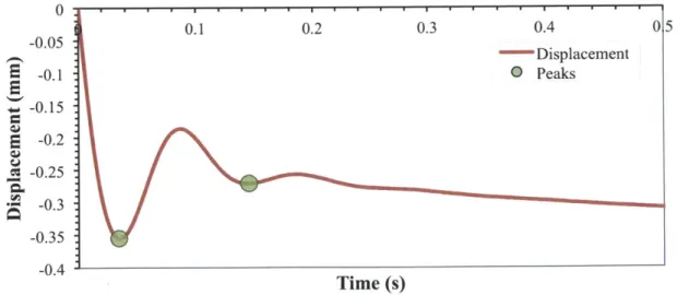
(im pact kinetic energy = 20.5 pJ) ... 55 Figure 3.26: Displacement profile from experiment on Gel 2 at impact velocity
vi. = 12.8 mm/s (impact kinetic energy = 17.6 pJ) showing the peaks ... 56
Figure 3.27: Schematic showing how the flat-punch indenter contacts the sample
surface edge-first... 57 Figure 3.28: Comparison of velocity profiles from experiment (without corrected
point of contact) and simulation for Gel 4 at impact velocity vi" = 4.1 mm/s
Figure 3.29: Comparison of displacement profiles from experiment (without corrected point of contact) and simulation for Gel 4 at impact velocity
vi. = 4.1 mm/s (impact kinetic energy = 1.8 pJ)... 58
Figure 3.30: Comparison of velocity profiles from experiment (with corrected point of contact) and simulation for Gel 4 at impact velocity vin = 4.1 mm/s
(im pact kinetic energy = 1.8 pJ) ... 59
Figure 3.31: Comparison of displacement profiles from experiment (with corrected point of contact) and simulation for Gel 4 at impact velocity
vi. = 4.1 mm/s (impact kinetic energy = 1.8 [J)... 59
Figure 4.1: (a) Storage modulus, (b) Loss modulus and (c) Loss tangent of Solvent A and Solvent B (Experimental data acquired by ARL collaborators,
J. Lenhart and R. M rozek) ... 62
Figure 4.2: Optimization of network phase against rat heart tissue with 60%
Solvent A (Experimental data acquired by Dr. I. Kalcioglu, Van Vliet Group)... 63
Figure 4.3: Optimization of network phase against rat heart tissue with 70%
Solvent A (Experimental data acquired by Dr. I. Kalcioglu, Van Vliet Group)... 63 Figure 4.4: Optimization of network phase against rat heart tissue with 80%
Solvent A (Experimental data acquired by Dr. I. Kalcioglu of Van Vliet Group)... 64 Figure 4.5: Optimization of network phase against rat heart tissue with 50%
Solvent B (Experimental data acquired by Dr. I. Kalcioglu of Van Vliet Group) ... 64
Figure 4.6: Optimization of network phase against rat heart tissue with 60%
Solvent B (Experimental data acquired by Dr. I. Kalcioglu, Van Vliet Group)... 64
Figure 4.7: Optimization of network phase against rat heart tissue with 70%
Solvent B (Experimental data acquired by Dr. I. Kalcioglu, Van Vliet Group)... 65 Figure 4.8: Optimization of network phase against rat heart tissue with 80%
Solvent B (Experimental data acquired by Dr. I. Kalcioglu, Van Vliet Group)... 65 Figure 4.9: (a,b) Storage modulus, (c,d) Loss modulus and (e,f) Loss tangent
of heart-optimized network phases for different volume fractions of Solvents
A and B (Experimental data on solvents acquired by ARL collaborators,
J. Lenhart and R. M rozek) ... 66 Figure 4.10: Comparison of normalized mean squared error NMSE for gels
velocity vi = 8.4 m m /s)... 69
Figure 4.11: Comparison energy dissipation capacity K for gels with Solvent
Figure 4.12: Comparison of quality factor
Q
for gels with Solvent A optimizedagainst rat heart tissue (Impact velocity vin = 8.4 mm/s)... 69 Figure 4.13: Comparison of maximum penetration depth xax for gels with
Solvent A and Solvent B optimized against rat heart tissue (Impact velocity
vin = 8.4 m m /s)... 69 Figure 4.14: Comparison of displacement profiles for impact velocity
Vin = 8.4 mm/s of the best heart-optimized gels and the rat heart tissue
(Experimental data acquired by Dr. I. Kalcioglu, Van Vliet Group)... 70
Figure 4.15: Optimization against rat liver tissue for 60% Solvent A
(Experimental data acquired by Dr. I. Kalcioglu, Van Vliet Group)... 71
Figure 4.16: Optimization against rat liver tissue for 70% Solvent A
(Experimental data acquired by Dr. I. Kalcioglu, Van Vliet Group)... 71
Figure 4.17: Optimization against rat liver tissue for 60% Solvent B
(Experimental data acquired by Dr. I. Kalcioglu, Van Vliet Group)... 72
Figure 4.18: Optimization against rat liver tissue for 70% Solvent B
(Experimental data acquired by Dr. I. Kalcioglu, Van Vliet Group)... 72
Figure 4.19: Optimization against rat liver tissue for 90% Solvent B
(Experimental data acquired by Dr. I. Kalcioglu, Van Vliet Group)... 72 Figure 4.20: (a,b) Storage modulus, (c,d) Loss modulus and (e,f) Loss tangent
of and liver-optimized network phases for different volume fractions of Solvents
A and B (Experimental data on solvents acquired by ARL collaborators,
J. Lenhart and R . M rozek) ... 73 Figure 4.21: Comparison of normalized mean squared error NMSE for the
optimized gels with Solvent A and Solvent B against rat liver tissue (Impact
velocity vi, = 8.2 m m /s)... 75
Figure 4.22: Comparison of energy dissipation capacity K for the optimized gels with Solvent A and Solvent B against rat liver tissue (Impact velocity
Vin '= 8.2 m m /s)... 75 Figure 4.23: Comparison of quality factor
Q
for the optimized gels with SolventA against rat liver tissue (Impact velocity vi, = 8.2 mm/s)... 76 Figure 4.24: Comparison of maximum penetration depth xma for the optimized
gels with Solvent A and Solvent B against rat liver tissue (Impact velocity
Figure 4.25: Comparison of displacement profiles for impact velocity vin = 8.2 mm/s of the best liver-optimized gels and the rat liver tissue
(Experimental data acquired by Dr. I. Kalcioglu, Van Vliet Group)... 77
Figure 4.26: Storage modulus of liver and heart tissues compared with that
of Solvent A, network phases of impact-optimized tissue simulant gels and network phases of ARL-fabricated gels of different stoichiometric ratios. The optimization of the network phases was done so that the composite tissue simulant gel, which contained 60% Solvent A, matched the impact characteristics of corresponding tissue. The ARL-fabricated gels also had 60% Solvent A
before the solvent was extracted to obtain the dry network phase. (Experimental data on network phases of ARL-fabricated gels acquired by Dr. R. Mahmoodian, Van Vliet Group. Experimental data on solvent acquired by ARL collaborators,
J. Lenhart and R. Mrozek. Experimental data on rat heart and liver tissues
acquired by Dr. I. Kalcioglu [12]) ... 78 Figure 4.27: Loss modulus of liver and heart tissues compared with that of
Solvent A, network phases of impact-optimized tissue simulant gels and network phases of ARL-fabricated gels of different stoichiometric ratios. The optimization of the network phases was done so that the composite tissue simulant gel, which contained 60% Solvent A, matched the impact characteristics of corresponding tissue. The ARL-fabricated gels also had 60% Solvent A before the solvent was extracted to obtain the dry network phase. (Experimental data on network phases of ARL-fabricated gels acquired by Dr. R. Mahmoodian, Van Vliet Group. Experimental data on solvent acquired by ARL collaborators, J. Lenhart and R. Mrozek. Experimental data on rat heart and liver tissues acquired by
Dr. I. Kalcioglu [12])... ... ... ... 79 Figure 4.28: Loss tangent of liver and heart tissues compared with that of
Solvent A, network phases of impact-optimized tissue simulant gels and network phases of ARL-fabricated gels of different stoichiometric ratios. The optimization
of the network phases was done so that the composite tissue simulant gel, which contained 60% Solvent A, matched the impact characteristics of corresponding tissue. The ARL-fabricated gels also had 60% Solvent A before the solvent was extracted to obtain the dry network phase. (Experimental data on network phases of ARL-fabricated gels acquired by Dr. R. Mahmoodian, Van Vliet Group. Experimental data on solvent acquired by ARL collaborators, J. Lenhart and R. Mrozek. Experimental data on rat heart and liver tissues acquired by
D r. I. K alcioglu [12])... 80
Figure 4.30: Storage modulus of liver and heart tissues compared with that of
Solvent B, network phases of impact-optimized tissue simulant gels and network phases ARL-fabricated gels of different stoichiometric ratios. The optimization of the network phases was done so that the composite tissue simulant gel, which contained 60% Solvent B, matched the impact characteristics of corresponding tissue. The ARL-fabricated gels also had 60% Solvent B before the solvent was extracted to obtain the dry network phase. (Experimental data on network phases
of ARL-fabricated gels acquired by Dr. R. Mahmoodian, Van Vliet Group. Experimental data on solvent acquired by ARL collaborators, J. Lenhart and R. Mrozek. Experimental data on rat heart and liver tissues acquired by
D r. I. K alcioglu [12])... 81
Figure 4.31: Loss modulus of liver and heart tissues compared with that of Solvent B, network phases of impact-optimized tissue simulant gels and network
phases ARL-fabricated gels of different stoichiometric ratios. The optimization of the network phases was done so that the composite tissue simulant gel, which contained 60% Solvent B, matched the impact characteristics of corresponding tissue. The ARL-fabricated gels also had 60% Solvent B before the solvent was
extracted to obtain the dry network phase. (Experimental data on network phases of ARL-fabricated gels acquired by Dr. R. Mahmoodian, Van Vliet Group. Experimental data on solvent acquired by ARL collaborators, J. Lenhart and R. Mrozek. Experimental data on rat heart and liver tissues acquired by
D r. I. K alcioglu [12])... 82
Figure 4.32: Loss tangent of liver and heart tissues compared with that of Solvent B, network phases of impact-optimized tissue simulant gels and network phases ARL-fabricated gels of different stoichiometric ratios. The optimization of the network phases was done so that the composite tissue simulant gel, which contained 60% Solvent B, matched the impact characteristics of corresponding tissue. The ARL-fabricated gels also had 60% Solvent B before the solvent was extracted to obtain the dry network phase. (Experimental data on network phases of ARL-fabricated gels acquired by Dr. R. Mahmoodian, Van Vliet Group. Experimental data on solvent acquired by ARL collaborators, J. Lenhart and R. Mrozek. Experimental data on rat heart and liver tissues acquired by
LIST OF TABLES
Table 3.1: PDMS gel designation and composite parameters ... 35
Table 3.2: Prony series parameters for network and solvent phases of Gel 1
(Data acquired by Dr. R. Mahmoodian, Van Vliet Group) ... 36
Table 3.3: Prony series parameters for network and solvent phases of Gel 2
(Data acquired by Dr. R. Mahmoodian, Van Vliet Group) ... 37 Table 3.4: Prony series parameters for network and solvent phases of Gel 3
(Data acquired by Dr. R. Mahmoodian, Van Vliet Group) ... 38
Table 3.5: Prony series parameters for network and solvent phases of Gel 4
(Data acquired by Dr. R. Mahmoodian, Van Vliet Group) ... 39
Table 3.6: Prony series parameters for composite Gel 1 (Data acquired by
Dr. R. Mahmoodian, Van Vliet Group)... 42
Table 3.7: Prony series parameters for equivalent Digimat material for Gel 1 ... 42 Table 4.1: Solvent designation and molecular weights... 62
Table 4.2: Prony series parameters for Solvents A and B (Data acquired by
Dr. R. M ahmoodian, Van Vliet Group)... 62
Table 4.3: Prony series parameters for heart-optimized network phases
(for different volume fractions of Solvent A)... 67 Table 4.4: Prony series parameters for heart-optimized network phases
(for different volume fractions of Solvent B)... 68 Table 4.5: Prony series parameters for liver-optimized network phases
(for different volume fractions of Solvent A)... 74
Table 4.6: Prony series parameters for liver-optimized network phases
Chapter 1: Introduction
1.1 Research Motivation
A tissue simulant is a synthetic material that mimics the mechanical response of
biological tissues, for example in response to impact loading. The design of more effective bulletproof vests and better protective armor is imperative to increasing the survivability of soldiers in the field. This requires the capability to accurately test the performance of such defensive systems against various impact forces due to blasts, bullets and other projectiles. In such experiments, tissue simulant materials are necessary as stand-ins for different types of living tissue, such as heart, liver and brain tissues, so that the effect of ballistics on such tissues can be analyzed with and without protective overlays. Tissue simulant materials are also useful in understanding mechanisms of injuries such as blunt force trauma and penetrative wounds [1].
For several decades, "ballistic gelatin" has been used as a tissue simulant as an alternative to animal tissues and cadavers. Produced by dissolving gelatin powder in water, it is inexpensive and commercially available, and approximates the density and viscosity of human muscle tissue. However its mechanical properties are very dependent on temperature and method of preparation, and will change over a period of a few days due to dehydration. It also does not exhibit a wide range of stiffhess that can simulate other tissues such as internal organs [2].
Recent works in developing better alternatives to ballistic gelatin have considered polymer-based gels like the commercially available Perma-GelTM and physically associating gels such as styrenic block copolymers [3-4]. Such polymer gels have mechanical properties that are more environmentally stable [5] as well as more tunable
easily deformable, while the crosslinked polymer allows the gel to recover elastically from any applied strain [8]. The tunability of the polymer gel arises from the possibility of using different polymer crosslinking ratios, solvent loadings and solvent molecular weights [9].
In the present study, the polymer gels considered are poly (dimethyl) siloxane (PDMS)
[10] gel systems developed by Dr. Joseph L. Lenhart et al. at the Army Research
Laboratory (ARL). They consist of a chemically crosslinked PDMS network and a non-reactive methyl-terminated PDMS solvent (Figure 1.1c). Several PDMS samples were synthesized at ARL by varying the stoichiometric ratio of crosslinking tetrafunctional tetrakis(dimethyl siloxy)silane groups (Figure 1.1b) to the vinyl-terminated PDMS precursor (Figure 1.1 a), the solvent molecular weight and the solvent loading percentage
[11], and the microscale mechanical behavior of such gels was analyzed experimentally
at MIT by Dr. Ilke Kalcioglu of the Van Vliet Group [12].
( a ) a a
c -P M
H2C=-Si- Si-O Si-O=CH2 NOW"
H I )/ IH vrf~em D OH H 3 CHy OMS
(b)
H cH3-Si-CH3 CH3 0 CH3 I I I ttafuncilonalH-SI-O-SI-0-Si-H suae cros-nker
I I I CH3 0 CH3 cH3-Si-CH 3 (c) OH3 OH3 OH3 I 1 1I40
H3C-Si- Si-O Si-CH3 non-reactive
I I I 11hy-e iad PDMS
CH3 LIM )nL
Figure 1.1: Chemical structures of the PDMS gel network components (a)
vinyl-terminated PDMS precursor, (b) tetrakis(dimethyl siloxy) silane crosslinker, (c) methyl-terminated non-reactive PDMS solvent (Image from [11])
The mechanical behavior of tissues and potential tissue simulants have been studied by different experimental methods [6,13,14,15,16], both quasi-static and dynamic. For the purpose of testing and developing tissue simulant materials, it is important that both the hydrated soft tissues as well as the potential tissue simulants are studied under similar ambient and loading conditions. It is also necessary that the loading conditions and the type of mechanical behavior studied are relevant to the purpose of the tissue simulant. To that end, and for the purpose of developing tissue simulant gels for ARL purposes, high-rate pendulum-based impact indentation experiments were conducted by Dr. I. Kalcioglu (Van Vliet Group) on polymer gels and heart and liver tissues [17]. This technique, developed by Constantinides et al., enabled the characterization of impact energy dissipation and resistance to penetration of the tissues and gels under localized impact loading conditions [18-19].
By this experimental approach, Dr. I. Kalcioglu (Van Vliet Group) quantified and
compared the mechanical characteristics of the candidate tissue simulant gels manufactured by ARL collaborators and provided information on which gels behave more similarly to rat tissues. This process involved providing feedback to the ARL about what parameters could be modulated to make the gels more comparable to tissues, and then repeating the experiments on newly prepared gels to validate such empirical predictions.
The present work is an effort to improve the efficiency of this process by implementing a computational model of the impact indentation experiment, so that the properties of the potential tissue simulant can be predicted and optimized. This would give material scientists a better idea of how to make such simulant gels, and reduce efforts in creating several gels and testing them experimentally. These data and approach can also provide basic correlations between composition and design of gels with tunable mechanical energy dissipation, including under mechanical loading conditions not accessible easily via experiment.
1.2 Multiscale Material Modeling
In the current study, the impact indentation experiment is modeled using finite element analysis. A macroscale finite element model, however, would consider the material as homogenous at the macroscopic level. Such an assumption would not accurately capture the behavior of a composite PDMS gel, which is affected by the heterogeneities in its microstructure including fluid-solid interactions. On the other hand, it is not conceivable to include the microstructure in the finite element model directly either, since that would
involve an exceptionally fine mesh and impractical computational resources. A compromise between these two approaches is to use a multiscale model.
In the multiscale method, we consider the macroscale and the microscale. The macroscale is the scale of the finite element model, and the microscale is the scale of the material microstructure, which usually consists of distinguishable matrix and inclusion phases [20]. In the case of the PDMS gels, the crosslinked PDMS network is considered the matrix and the PDMS solvent is taken as the inclusion.
At the macroscale, the composite material is represented by a finite element mesh that is locally homogenous, and at each mesh computation point (node), the microstructure is taken into account using the concept of a Representative Volume Element (RVE), a statistically representative sample of the material (Figure 1.2). Its size is much smaller than the macroscale material dimensions but it is large enough to capture microstructural properties like volume fraction and aspect ratio of the inclusion, and material properties of the multiple phases [21].
Finite Element Mesh
Matrix
10 (crosslinked
0
g
PDMS)Computation Point Incluson
solvent)
Macroscale ( ) Microscale
Figure 1.2: Representation of multiscale model
At each computation point of the mesh, the macroscale strain or stress values are used as the boundary conditions for the RVE, and the volume average of the stress or strain fields in the RVE is taken as the effective macroscopic response of the material at that point. This transition from the heterogeneous microscale-level of the RVE to the effective properties of the macroscale homogeneous material is done by scale-transition methods, such as generalized method of cells [22], asymptotic homogenization [23], direct finite element analysis of the RVE and mean-field homogenization [24]. The last of these, which is computationally efficient, is used in the present study.
The most accurate method of solving the RVE is to model the microstructure using finite element analysis (FEA) to obtain the detailed stress and strain fields within the RVE. However, meshing a complex microstructure can be troublesome and using FEA to solve the RVE at each computation point of the macroscale model would be computationally expensive, especially for non-linear elastic materials [25]. A more economical approach is mean-field homogenization (MFH), where each inclusion and the matrix are treated as separate domains, and only the average values of the stress/strain fields in these subdomains are computed rather than the detailed fields. It is generally assumed that the each domain behaves according to the macroscopic constitutive relations of the corresponding phase material [26].
Different MFH schemes exist, most based on Eshelby's solution [27] of a single ellipsoidal inclusion in an infinite elastic matrix. They differ in their derivations of the concentration tensors, which relate the stress/strain fields of the matrix and inclusions
[28]. For example, in the Mori-Tanaka (M-T) scheme, which extends the Eshelby's
solution, it is assumed that each inclusion behaves as if it were isolated in an infinite matrix and the matrix average stress/strain is applied as the boundary condition to the inclusion [29]. The M-T model is noteworthy for predicting the effective properties of two-phase composites, especially at low or high inclusion volume fractions [26].
Another family of MFH schemes is realized by the Double-Inclusion (D-I) model, proposed by Hori and Nemat-Nasser [30], which assumes that each inclusion is enclosed in another inclusion of matrix material and this double-inclusion is embedded in an infinite unknown material. Setting the unknown material as the matrix material, the D-I model collapses to the M-T model, whereas setting it as the inclusion material gives us the Inverse M-T model [31]. The Lielens model, also known as the Interpolative D-I model, interpolates the unknown material between the M-T and Inverse M-T models, and gives good results for intermediate inclusion volume fractions [32]. The Self-Consistent
(S-C) model assumes that the unknown material is a homogeneous material equivalent to
the heterogeneous composite [33]. The S-C model was developed for polycrystals and is not as well suited for two-phase composites [31]. Most of these MFH schemes have been tested against direct FEA simulations of RVEs and have been extended to multi-phase inelastic composites as well, although there is still scope for advancement in the non-linear regime [34].
Once a homogenization method is decided upon, there are two ways of implementing the multiscale model: sequential and concurrent. In the sequential approach, the microscale model is first analyzed to obtain the equivalent macroscopic behavior of the composite
and then the macroscale model is solved using the properties of this equivalent material. In the concurrent approach, both the microscale and the macroscale models are executed simultaneously [35]. At each time step and mesh point of the macroscale model, the RVE is solved using the current macroscopic stress/strain as the boundary condition, and this
response of the RVE is used in the next time step of the macroscale analysis. This coupling allows for a more accurate prediction of the macroscopic response of the
composite due to its microscopic heterogeneities, and is implemented in the present work.
1.3 Thesis Organization
This thesis is organized as follows:
Chapter 1 included the motivation for this research and introduced multiscale modeling, which is used to analyze the polymer gels.
Chapter 2 describes the impact indentation experiment and the finite element model developed to simulate this experiment.
Chapter 3 introduces the parameters used to characterize the energy dissipation and the resistance to penetration of the different tissue and gel samples. The simulated data from the computational model are compared to the experimental data using these parameters. The limitations of the computational model are also discussed.
Chapter 4 describes how the computational model can be used to predict the material properties of tissue simulant gels, and presents the results of such optimization in the case
of heart and liver tissues.
Chapter 2: Multiscale Model
The experimental setup described in Section 2.1 was used by Dr. I. Kalcioglu (Van Vliet Group) to conduct her experimental analysis on tissues and candidate tissue simulant gels. The multiscale material modeling approach described in Section 2.2.3 was suggested by Dr. R. Mahmoodian (Van Vliet Group) for the purpose of this project and she also contributed to the implementation of the Digimat-Abaqus interface.
2.1 Experimental Setup
Figure 2.1 shows a schematic of the experimental apparatus used by Dr. I. Kalcioglu
(Van Vliet Group) in her experiments, a commercially available pendulum-based instrumented indenter (NanoTest, Micro Materials, Wrexham, UK). The pendulum is fixed to the support frame through a pivot in the middle and it is free to rotate frictionless about this pivot. A flat punch or spherical indenter is rigidly attached to the pendulum, below the pivot, so that it can swing towards the sample, which is mounted vertically near the indenter [18-19].
The instrument was modified by adding a liquid cell to the sample mount (Figure 2.2), so that the tissue and gel samples could be tested in a fluid immersed state, which ensured that they were fully hydrated [36].
The impact force on the indenter is applied through an electromagnetic voice coil that interacts with the top of the pendulum. A parallel plate capacitor mounted on the pendulum in the same horizontal plane as the indenter is used to measure the displacement of the indenter. At the bottom of the pendulum, a pyramid of magnetically soft iron is attached, so that the pendulum can be attracted away from the sample by switching on the current in a nearby solenoid. The entire setup is housed in an acoustic
isolation enclosure at a controlled temperature (260 C) and relative humidity (50%), to reduce any vibrations or changes in ambient conditions [18-19].
Figure 2.1: Experimental setup (Image from [18])
displacement capacitor t --- force pendulum indenter mount liquid/air interface sample sample backplate removable plate mount liquid cell
For applying an impact load to the indenter, the solenoid at the bottom is first energized so that it pulls and holds the pendulum away from the sample. The sample plate is then moved in the direction of the indenter so that the sample surface is brought to the contact plane, which is 0.5 mm away from the vertical equilibrium plane of the free pendulum. A constant current, which determines the impact force, is then applied through the electromagnetic coil at the top and is maintained throughout the test. The solenoid is then shut off to release the pendulum, so that the indenter impacts the sample. The displacement trajectory of the indenter is recorded by the capacitor as a function of time. The velocity profile is obtained by differentiating the displacement curve. Figures 2.3 and 2.4 show example displacement and velocity profiles respectively obtained from an experimental run on a PDMS gel. The time is zero when the indenter makes contact with the material. The zero displacement corresponds to the point of contact at the material surface, and the negative direction is the penetration direction into the material from its free surface. 0 . . . .. . . --0.05 -!.1 0.2 0.3 0.4 0 5 -0.1 -0.15 c -0.2 .4 -0.25 -0.3 Time (s)
Figure 2.3: Example displacement profile from experiment on a PDMS gel
10 . 5 0 10.2 0.3 0.4 0 5 S-10 -15 Time (s)
2.2 Finite Element Model
The commercially available finite element analysis software Abaqus was used to create a computational model of the experimental setup described in Section 2.1.
2.2.1 Mesh, Indenter and Contact Formulation
The sample sizes of gel or tissue used for testing were approximately 5-6 mm thick, 15-20 mm in length and 10-13 mm in width. A flat punch of radius 1 mm was used for testing the PDMS gels. Since the length and width are much larger compared to the contact area of the punch, the sample dimensions were approximated as a cylindrical disc of radius 10 mm and thickness 5 mm. In this way, the symmetrical nature of the indenter loading was taken advantage of, and an axisymmetric mesh of the gel sample was created. Compared to three-dimensional (3D) elements, axisymmetric elements significantly reduce the problem size and the computational resources required [37].
Figure 2.5 shows the axisymmetric mesh used to represent the polymer gel sample being tested. The element spacing was created such that the mesh is more refined near the central region where the indenter impacts the material, and coarser away from this region. The element type used was CAX4, which is a 4-node bilinear axisymmetric quadrilateral solid element [38].
A mesh convergence study (Figure 2.6) was performed so that the optimal number of
elements could be used. This ensured that the mesh would accurately represent the problem while being computationally efficient. The number of elements chosen was 9750. 0.535 0.53 0.525 ,~0.52 0.515 0.51 - 0.505
Number of elements chosen = 9750
0.5
0.495
0 20000 40000 60000 80000 100000 120000 140000
Number of elements in mesh
Figure 2.6: Mesh convergence study
The flat punch indenter was modeled as an analytical rigid surface. Since the indenter is made of a much harder material (stainless steel) than the sample and it would undergo negligible deformation within itself, modeling it as a rigid body was a natural choice. An analytical rigid surface was used since it allows the axisymmetric profile of the indenter to be defined using a series of line segments or curves. The motion of an analytical rigid surface in Abaqus is governed by the motion of its reference node, and its mass and inertial properties are associated with this single reference node. Analytical rigid surfaces
are better suited to contact modeling than rigid surfaces composed of elements because they are single-sided and greatly reduce the computational cost [39].
In the experiment, the indenter is fixed to the pendulum and its motion is governed by the forces on this pendulum. The pendulum has a spring constant, k = 10 N/m and damping
coefficient, c = 0.96 Ns/m [18-19]. The pendulum mass along with the weight of the fluid extension and the flat punch, m = 0.215 kg were applied to the reference node of the analytical indenter surface. The pendulum action was modeled as spring-damper system, with the specified k and c values, attached to the indenter on one end and a fixed point at the other end, as shown in Figure 2.7.
The contact interaction is modeled between the indenter surface and the top surface of the sample, using a node-to-surface contact discretization and small-sliding tracking approach. The node-to-surface discretization ensures that the indenter surface does not penetrate through the surface of the material and it is also less computationally intensive than the surface-to-surface discretization. The small-sliding approach also saves computational cost and it assumes that there will be little relative sliding between the two contact surfaces [40]. The friction in the contact formulation is set to zero, as it is assumed that friction is negligible in the interaction between the indenter and the material.
2.2.2 Loading
The impact loading on the spring-indenter system is applied in three steps. Initially, at Step Zero (Figure 2.9a), the indenter is at rest, just making contact with the surface of the gel and the spring is relaxed. In Step One (Figure 2.9b), an initial compressive displacement Xeq of 0.5 mm is imposed on the spring by applying a suitable force at the
top end of the spring. This was done to be consistent with the experiment, where the contact between the indenter and sample occurs in a plane 0.5 mm from the vertical equilibrium plane (Figure 2.8). Therefore the pendulum still has some potential energy when contact occurs, and this is equivalent to the potential energy added to the spring by the compression in this step. The top end of the spring is maintained fixed after this step.
Pendulum Plane of vertical
equilibrium of pendulum
Flat-punch indenter
Sample Plane of sample surface
(Plane of contact)
0.5 mm (x q)
In Step Two (Figure 2.9c), the indenter is moved away from its initial position of contact with the material. This is equivalent to the experimental action where the pendulum is moved away from the sample before impact. Before running the final simulation, the distance by which the indenter is moved away is adjusted, by iteratively changing the upward force
fp
applied on the indenter in this step, until the velocity vi, with which the indenter impacts the material in Step Three matches the impact velocity reported in the experiment. This calibrated forcefp, is used in the final simulation used for analysis.(a) Step Zero (b) Step One
(c) tep Iwo (d) Step Three
Step Three (Figure 2.9d) is a Dynamic step where the spring-indenter system is released from its compressed state. A constant force
f
4,, is also applied on the indenter, which is equal to the constant force applied to the pendulum in the experiment. In this way, the impact force and impact velocity values are made consistent between the experiment and the simulation. The displacement and the velocity in the axial direction at the indenter reference node are obtained from this step and these are compared to the displacementand velocity profiles from the experiment.
2.2.3 Material Definition
The simulations were run for various PDMS gels that had previously been tested experimentally. These gels are composed of two viscoelastic phases, a chemically crosslinked network of PDMS and a non-reactive PDMS solvent. The effective macroscopic response of this two-phase viscoelastic composite was captured with the help of the commercially available multiscale material modeling software, Digimat.
The Digimat software has the option of using several modules. Sequential multiscale modeling can be implemented through Digimat-MF, a mean field homogenization module, and Digimat-FE, a direct finite element analysis module. The one most suited to the current study however, is the Digimat-CAE module, which uses concurrent multiscale modeling and interfaces between Digimat-MF/FE and the macroscale analysis software. Instead of computing the overall properties of the composite material in the beginning of the analysis and keeping them constant throughout the Abaqus simulation, Digimat-CAE calculates the changing material properties of the composite at each iteration. Thus Abaqus and Digimat are in constant communication with each other throughout the simulation, with Digimat supplying the material definition at each integration point and at each time step, and Abaqus supplying the current load and stress state of the material for Digimat to update its computation [20]. Digimat-MF offers Mori-Tanaka, Double-Inclusion and Multi-inclusion homogenization schemes. The Mori-Tanaka model was found to be well suited for our PDMS gels.
The properties of the two viscoelastic phases of the microstructure are represented by a Prony series. The Prony series is based on the Generalized Maxwell model of viscoelasticity, which uses several spring and dashpot elements to represent the elastic and viscous behaviors of the material respectively. As opposed to the Maxwell model, which only uses one spring and one dashpot element, this model takes into account that viscoelastic materials consist of molecular segments of varying lengths contributing to varying relaxation times.
The Prony series for the shear stress relaxation modulus is:
G(t) =Go - Z% 1 Gi 1 - e Thi --- Equation 2.1
where Go = G(t=O) is the elastic shear modulus.
Normalizing Eq. 2.1 by Go, we obtain the dimensionless shear stress relaxation modulus as:
g(t) = G = =1 - Li gi 1 - e t/Ti --- Equation 2.2
where N, gi = G and -ri are material constants which can be obtained by curve-fitting
Go
Eq. 2.2 to experimental data obtained from a stress relaxation test on the material.
The Prony series used to represent the material phases in the present study were calculated from the shear storage modulus (G9 and shear loss modulus (G'9 obtained from rheological tests. The rheological experiments on the solvent phases were conducted
by the ARL and those on the solvent-extracted matrix phases by Dr. Roza Mahmoodian
of the Van Vliet Group. The extraction of the solvent from the gels to obtain the matrix phases for testing was performed by Wen Shen of the Van Vliet Group. Appendix Al describes this solvent extraction procedure in detail.
The shear storage and shear loss moduli are represented in terms of Prony series parameters as follows [41]:
The number of terms in the series N is assumed and initial estimates for parameters Go, gi and r are used to calculate G'(w) and G"(w) using Equation 2.3 and Equation 2.4. The least square errors between these calculated values and the experimental values are then minimized by a MATLAB optimization algorithm to get the values of the Prony series parameters. The number of Prony series terms N was assumed as 10, which was an optimal number to capture the viscoelastic nature of the range of gel phases used in the study. Appendix A2 contains the MATLAB code written by Dr. R. Mahmoodian (Van Vliet Group) to calculate the Prony series from the rheology data.
Chapter 3: Validation of Model
The computational model was validated by running simulations of impact indentation on four PDMS gel samples fabricated by the ARL, and comparing their energy dissipation characteristics with those obtained from the experiments run by Dr. I. Kalcioglu (Van Vliet Group). The viscoelastic properties of the solvent and network phases of the gels as well as the volume fraction of the phases were used as the material input for Digimat. The Prony series used to represent the viscoelastic nature of the phases were obtained by Dr. R. Mahmoodian (Van Vliet Group) by the method described in Section 2.2.3.
Table 3.1 describes the parametric features of the four composite polymer gels used for validation. These gels were chosen because they were the least sticky of all the fabricated samples, reducing the effects of adhesion in the experiment. This was an important criterion since adhesion was not modeled in the simulation.
Designation Solvent Solvent Solvent Network Stoichiometric
used in Molecular designation Volume Volume ratio of
present Weight used in Fraction Fraction network phase
work (kg/mol) [7], [11] (%) (%) (silane:vinyl)
Gel 1 308 T308 50 50 4:1
Gel 2 308 T308 60 40 4:1
Gel 3 139 T139 60 40 4:1
Gel 4 139 T139 60 40 3:1
Table 3.1: PDMS gel designation and composite parameters
Tables 3.2 - 3.5 detail the Prony series parameters (Go, gi, ri) of the network and solvent phases of the four composite PDMS gels. The dynamic modulus of the network and solvent phases of these gels calculated from the Prony series using Equations 2.3 and 2.4
(a)
.. Network phase (50%, 4:1) Solvent phase (308 kg/mol)
1.E+05 1.E+04 PC1.E+03 1.E+02 I.E+01 1.E+00 0 2 1.0 0.8 0.6 ,0.4 0.2 0.0 Frequency f (Hz) 8 10 1.E+05 1.E+04 1.E+03i 1.E+02 1.E+0 I I.E+J 0 2 4 6 8 10 12 Frequencyf (Hz) 0 - - . . . . . 0 2 4 6 8 10 12 Frequencyf (Hz)
Network phase Solvent phase
(50%, 4:1) (308 kg/mol) Go = 92.962 kPa Go = 189.64 kPa ri (S) gi Ti (S) g, 0.0100 0.0554 0.0100 0.6761 0.0278 0.1368 0.0373 0.0747 0.0774 0.0646 0.1390 0.2325 0.2154 0.0942 0.5180 0.0030 0.5995 0.0709 1.9307 0.0127 1.6681 0.0620 4.6416 0.0507 12.915 0.0341 35.938 0.0221 100.00 0.0381
Figure 3.1: (a) Storage modulus, (b) Loss
modulus and (c) Loss tangent of network and
solvent phases of Gel 2 (Experimental data
on solvent phase acquired by ARL
collaborators, J. Lenhart and R. Mrozek. Experimental data on network phase acquired by Dr. R. Mahmoodian, Van Vliet
Group)
Table 3.2: Prony series parameters
for network and solvent phases of Gel 1 (Data acquired by Dr. R.
Mahmoodian, Van Vliet Group) (b)
Solvent phase (308 kg/mol)
(C)
Network phase (50%, 4:1) Solvent phase (308 kg/mol)
r
4 6 Frequencyf (Hz) 4 6 Frequencyf (Hz) 8 8 1.E+05 I.E+0U 10 10 0 2 4 6 8 10 Frequencyf (Hz)
Network phase Solvent phase
(40%, 4:1) (308 kg/mol) Go = 125.96 kPa Go = 189.64 kPa Ti (S) 9i ri (S) gj 0.0100 0.0001 0.0100 0.6761 0.0316 0.2006 0.0373 0.0747 0.1000 0.0969 0.1390 0.2325 0.3162 0.0768 0.5180 0.0030 1.0000 0.0629 1.9307 0.0127 3.1623 0.0521 10.000 0.0385 31.623 0.0575
Figure 3.2: (a) Storage modulus, (b) Loss modulus and (c) Loss tangent of network and solvent phases of Gel 2 (Experimental data
on solvent phase acquired by ARL
collaborators, J. Lenhart and R. Mrozek. Experimental data on network phase acquired by Dr. R. Mahmoodian, Van Vliet Group)
Table 3.3: Prony series parameters for network and solvent phases of Gel 2 (Data acquired by Dr. R.
Mahmoodian, Van Vliet Group)
(a)
Network phase (40%, 4:1) Solvent phase (308 kg/mol)
, .E+04 wI .E+03 I.E+02 1.E+01 1.E+00 I.E+05 1.E+04 1.E+03 L.E+02 1.13+01
(b)
Network phase (40%, 4:1) Solvent phase (308 kg/mol)1-. 0.8 0.6 0.4 0.2 0 2 2 * X 0 0 C) Network phase (40%, 4: 1)
I.E+06 1.E+05 I.E+04 1.E+03 1.E+02 1.E+01 1.E+00
(a)
"Network phase (40%, 3: 1)-_1Solvent phase (139 kg/mol)
1.E-01 I. . . . . ... i 0 2 4 6 8 10 Frequencyf (Hz) 0.8 0.6 0.4 0.2 -0 0 2 4 6 Frequencyf (Hz) 8 1.E+06 I.E+05 1.E+04 1.E+03 1.E+02 I.E+01 1.E+00 I.E-01 10
Figure 3.3: (a) Storage modulus, (b) Loss modulus and (c) Loss tangent of network and solvent phases of Gel 3 (Experimental data on solvent phase acquired by ARL collaborators,
J. Lenhart and R. Mrozek. Experimental data
on network phase acquired by Dr. R. Mahmoodian, Van Vliet Group)
0 2 4 6 8 10
Frequencyf (Hz)
Network phase Solvent phase
(40%, 3:1) (139 kg/mol) Go = 125.96 kPa Go = 189.64 kPa Ti (s) g; r, (s) gi 0.0100 0.0190 0.0100 0.9327 0.0316 0.2314 0.0631 0.0615 0.1000 0.0677 0.3981 0.0057 0.3162 0.0804 1.0000 0.0591 3.1623 0.0521 10.000 0.0399 31.623 0.0588 100.00 0.0001
Table 3.4: Prony series parameters
for network and solvent phases
of Gel 3 (Data acquired by Dr. R. Mahmoodian, Van Vliet Group)
PC
rA rA
(b)
""Network phase (40%, 3:1) " Solvent phase (139 kg/mol)
(c)
Network phase (40%, 3: 1)
(a)
Network phase (40%, 4:1) "Solvent phase (139 kg/mol)
1.E+05 .. E+04 1.E+03 E I.E+02 1.E+01 1.E+00 LE-01 0 2 4 6 Frequencyf (Hz) 1.E+05 1 1.E+04 1.E+03 l.E+02 o I.E+01 I L.E+00 1 1.E-8 10 -. ... . . . ... . 0 2 4 6 8 10 Frequencyf (Hz) 1 .. ... ; . '. 0 2 4 6 8 1' Frequencyf (Hz)
Network phase Solvent phase
(40%, 4:1) (139 kg/mol) Go = 125.96 kPa Go = 189.64 kPa 0.0100 0.0001 0.0100 0.9327 0.0316 0.2006 0.0631 0.0615 0.1000 0.0969 0.3981 0.0057 0.3162 0.0768 1.0000 0.0629 3.1623 0.0521 10.000 0.0385 31.623 0.0575 0
Figure 3.4: (a) Storage modulus, (b) Loss
modulus and (c) Loss tangent of network and solvent phases of Gel 4 (Experimental data on solvent phase acquired by ARL collaborators, J. Lenhart and R. Mrozek. Experimental data on network phase acquired by Dr. R. Mahmoodian, Van Vliet
Group)
Table 3.5: Prony series parameters
for network and solvent phases of Gel 4 (Data acquired by Dr. R.
Mahmoodian, Van Vliet Group) I(b)
""Network phase (40%, :1) Solvent phase (139 kg/mol)
0.8 0.6 0.4 0.2 C' U, U, 0
(C)
" ,Solvent phase (139 kg/mol)Network phase (40%, 4:1l)
0
-I.E+06 I.E+06
3.1 Parameters of Comparison: K,
Q,
x,,,Three parameters were used to quantify the energy dissipation characteristics of the material (tissue or polymer gel). They were used for comparison between experimental
and simulated data.
1. Energy dissipation capacity, K
This is a measure of the energy dissipated during the initial impact of the indenter (Figure 3.5). It is defined as
K Energy dissipated by the material during the first impact cycle Energy input into the material during the first impact cycle
K =Ein - Eout - Edp Ein-Edp
1 2 1 Eu
Ei= mv + -kxinz, EDUt = tmnvout2 + kxut 2
22 2 2 t
in = Xeq - din, Xott = Xeq - dout
where m is the mass (in kg) and k is the spring constant (in N/m) of the pendulum or spring. vi, and v,., are the velocities (in m/s) of the indenter at the beginning and end of the first impact cycle, respectively. Hence the terms mvin2 and mout2 are the
kinetic energies (in J) of the indenter at the beginning and end of the cycle. In the experiment; xi, and x., are the distances (in m) between the equilibrium plane of the pendulum and the positions of the pendulum at the beginning and end of the first impact cycle. In the simulation, xi,, and x0,, correspond to the compressive displacement (in m) on the spring from its equilibrium state, at the beginning and end of the first impact cycle. Hence the terms 1 kxn2 and 1 kxut2 are the potential
energies (in J) of the indenter at the beginning and end of the cycle. In the experiment, xeq is the distance between the equilibrium plane of the pendulum and the
free surface of the sample. In the simulation, Xeq is the initial compressive displacement applied on the spring in Step One of loading (Section 2.2.2). di, and du,