HAL Id: halshs-01183166
https://halshs.archives-ouvertes.fr/halshs-01183166
Submitted on 6 Aug 2015HAL is a multi-disciplinary open access archive for the deposit and dissemination of sci-entific research documents, whether they are pub-lished or not. The documents may come from teaching and research institutions in France or abroad, or from public or private research centers.
L’archive ouverte pluridisciplinaire HAL, est destinée au dépôt et à la diffusion de documents scientifiques de niveau recherche, publiés ou non, émanant des établissements d’enseignement et de recherche français ou étrangers, des laboratoires publics ou privés.
Valuation of commodity derivatives with an
unobservable convenience yield
Anh Ngoc Lai, Constantin Mellios
To cite this version:
Anh Ngoc Lai, Constantin Mellios. Valuation of commodity derivatives with an
unobserv-able convenience yield. Computers and Operations Research, Elsevier, 2016, 66, pp.402-414.
Author's Accepted Manuscript
Valuation of Commodity Derivatives with an
Unobservable Convenience Yield
Anh Ngoc Lai, Constantin Mellios
PII:
S0305-0548(15)00065-9
DOI:
http://dx.doi.org/10.1016/j.cor.2015.03.007
Reference:
CAOR3747
To appear in:
Computers
& Operations Research
Cite this article as: Anh Ngoc Lai, Constantin Mellios, Valuation of Commodity
Derivatives with an Unobservable Convenience Yield, Computers & Operations
Research,
http://dx.doi.org/10.1016/j.cor.2015.03.007
This is a PDF file of an unedited manuscript that has been accepted for
publication. As a service to our customers we are providing this early version of
the manuscript. The manuscript will undergo copyediting, typesetting, and
review of the resulting galley proof before it is published in its final citable form.
Please note that during the production process errors may be discovered which
could affect the content, and all legal disclaimers that apply to the journal
pertain.
1
Valuation of Commodity Derivatives with an Unobservable Convenience Yield
Anh Ngoc Laia and Constantin Mellios b,1∗
a
Labex « Financial Regulation », University Rennes 1, IGR-IAE, 11 rue Jean Macé, CS 70803 35708 Rennes Cedex 7, France , e-mail address laianhngoc@yahoo.com
b, ∗ Corresponding author, PRISM-Sorbonne and Labex « Financial Regulation », University Paris 1 Panthéon-Sorbonne, 17,
place de la Sorbonne, 75231 Paris Cedex 05, France. Tel: + 33(0)140462807; fax: + 33(0)140463366. e-mail address: constantin.mellios@univ-paris1.fr !" #$%%&' ( ) * + !" a
Labex « Financial Regulation », University Rennes 1, IGR-IAE, 11 rue Jean Macé, CS 70803 35708 Rennes Cedex 7, France , e-mail address laianhngoc@yahoo.com
b, ∗ Corresponding author, PRISM-Sorbonne and Labex « Financial Regulation », University Paris 1 Panthéon-Sorbonne, 17,
place de la Sorbonne, 75231 Paris Cedex 05, France. Tel: + 33(0)140462807; fax: + 33(0)140463366. e-mail address: constantin.mellios@univ-paris1.fr
2
) , - - - -
-1. Introduction
In recent years, storable commodity markets (energy, agricultural, metals, etc.)2 booms and busts have revived the interest for commodity derivatives, which have been characterized by a dramatic growth in trading volume and by the proliferation of contracts written on a wide range of underlying commodities. Especially, according to the Bank of International Settlements (BIS), the notional value of over-the-counter (OTC) commodity derivatives stood at $2.6 trillion in 2012. In the US and in the European Union regulation in force has a significant impact on the commodities trading industry and on OTC contracts, in particular. This may have important implications on pricing, hedging and managing risk in commodity derivatives markets.
Not surprisingly, much literature has been devoted to the pricing and hedging of commodity derivatives. Reduced-form models turn out to be the appropriate models for such considerations. They try to identify the relevant state variables or factors associated with the dynamics of the futures prices. The stochastic processes of these variables are specified exogenously by taking into account some of
2
3
the specific features describing the behavior of commodities. Storable commodities, in contrast to other conventional securities, are real assets that can be produced and consumed. Thus holding physical inventories may provide some services in order to avoid shortages and therefore to maintain the production process or to respond to an unexpected demand, for example3. These services are qualified to as the convenience yield, when expressed as a rate (see, for example, the definition in [1]). The theory of storage ([2], [3], and [4]) has studied the relationship between commodity prices and storage decisions, and has established a no-arbitrage relation between futures prices, spot commodity prices, the interest rate and the net convenience yield. Moreover, a growing number of empirical studies on commodity return predictability pointed out the important role of the convenience yield especially (see, for instance, [5], [6], [7], [8], [9], and [10]). The spot price and the convenience yield are therefore the two commonly used state variables in pricing models.
It is widely recognized in the literature (see, for instance, [11]) that the convenience yield is not directly observable. Thus, when pricing commodity derivatives, a difficulty arises from this non-observability. Gibson and Schwartz [12] used the theory of storage formula to calculate the implied convenience yield. The latter can be inferred by using futures and spot prices (or the futures contract price closest to maturity as a proxy for the spot price if it is not available). However, prices may be
3
Gülpinar et al. [14], for instance, study the impact of supply disruptions in the oil market on portfolio management involving commodity derivatives.
4
subject to temporary mispricing or to liquidity concerns, for example. Carmona and Ludkovski [13] also showed that the implied convenience yield is unstable over time and incompatible with the forward curve. Using prices from futures contracts with different maturities will provide very different convenience yields. Dockner et al. [15] suggest a new analytical approximation of the convenience yield by computing the difference between the present values of two floating-strike Asian options written on the spot and the futures prices, respectively. They have found, however, that different approximation methods give rise to different convenience yield estimates. The differences can be attributed to the cost of carry and the moneyness of the options.
The main objective of this paper is to build a reduced-form valuation model of commodity forward and futures contracts as well as options on forward and futures contracts by explicitly taking into account the unobservable character of the convenience yield. Although many models dealing with a partially observable economy or with incomplete information have studied the unobservability of a stochastic expected return (see, for instance, [16], [17], and [18] for an application to interest rates and to asset allocation), to the best of our knowledge, the case of an application to commodities with a partially observable convenience yield has not been examined yet.A notable exception is Carmona and Ludkovski [19] who developed a utility-based pricing model resulting in a partially observable stochastic control problem.
5
The reduced-form models fall into two categories. In the first one, in addition to the spot price and the convenience yield (see [12], [20], [21], and Liu and Tang, [22]), other state variables and some stylized facts have been suggested in the literature. The interest rate ([11], [23], and [24]), the volatility of the spot price ([25], [26], [27], and Benth [28]), jumps in the spot price and the volatility ([23], [25], and Schmitz et al. [29]) or seasonal patterns in commodity prices ([26], [30], [31], and Back et al. [32]). Schwartz and Smith [33] have suggested a two-factor model allowing for a short-term mean reversion in spot prices toward a random long-short-term equilibrium level. To take into account some observed features of the convenience yield, Paschke and Prokopczuk [34] have generalized the Schwartz and Smith model by assuming that the short-term component follows a continuous autoregressive moving-average process. Garcia et al. [36] have developed a four-factor model to take into account mean reversion and stochastic seasonnality in the convenience yield. Cortazar and Naranjo [37] and Paschke and Prokopczuk [38] have developed multi-factor models to explain the random behavior of oil prices. The second category of the reduced-form models is inspired by the Heath et al. [39] model, which is consistent with the initial term structure of interest rates. It was pioneered by Miltersen and Schwartz [40] who built a model to price options on commodity futures, with a stochastic convenience yield, which is consistent with the initial term structures of both interest rates and commodity futures prices. Miltersen [41] have extended the Gibson and Schwartz [12] model in order to fit the initial term structure of forward and futures prices, as well as that of forward
6
and futures volatilities4. Trolle and Schwartz [42] have suggested a model to account for (unspanned) stochastic volatility of both the spot price and the instantaneous forward cost of carry. Manoliu and Tompaidis [43] have proposed a multi-factor model accounting for seasonal patterns in the futures curve.
The models mentioned above are constructed in a fully observable framework. They assume that the variables which describe the state of the economy are observable. However, some of the state variables, which are relevant to financial claims valuation, are generally not observable, the instantaneous convenience yield, in particular. Investors operate in an economic environment with incomplete information. The clarifying paper of Feldman [46] has judicially discussed several issues related to the incomplete information equilibrium. Dothan and Feldman [47], Detemple [48], Gennotte [49] and Xia [18], among others, have investigated, in a dynamic framework, the optimal asset allocation and asset valuation in a partially observable economy. In this economy, the agent estimates one or more unobserved state variable(s) given information conveyed by past observations. The estimation or filtering error represents the agent's assessment of the precision of the estimate and
4 This a direct analogue of the Hull and White [44] model which extended the Vasicek [45] model to fit the initial yield curve
7
reflects his (her) quality of information. The investor’s optimization problem is then based on the conditional mean(s), which also determine(s) contingent claims prices5.
In this article, we propose a three-factor model in an incomplete information setting in the spirit of the Schwartz [11] model 3, which is the reference model in the literature involving the convenience yield. In order to do so, the economic framework retains the spot commodity price, the instantaneous interest rate and the convenience yield as the relevant stochastic state variables associated with the dynamics of the futures price. Contrary to this model and to the other reduced-form models, the convenience yield is not observable, but investors can draw inferences about it by observing the spot commodity price and the short rate by using the continuous-time Kalman-Bucy filter method6.
From a theoretical point of view, our contribution to the literature is threefold. First, we extend the relevant literature by pricing derivatives under incomplete information7. This framework is well-adapted to the case of storable commodities since the convenience yield is unobservable. Second, in
5
Hernandez et al. [50] have suggested an alternative procedure, a moment method algorithm, to estimate the parameters of an unobservable stochastic mean and have applied it to commodities.
6
The Casassus and Collin-Dufresne [24] model allows the convenience yield to depend on the spot price and the interest rate, but in a fully observable economy.
7 See also Mellios [35] who has developed a model to price European-style interest rate options in a partially observable
8
sharp contrast to models in a partially observable economy, we provide simple closed-form solutions for forward and futures prices, as well as for European options on forward and futures contracts. Thus our model inherits this appealing feature of fully observable reduced-form models with a Gaussian structure facilitating its use for practical considerations. Also, two-factor and one-factor models can be easily derived. Third, these analytical solutions allow one to examine the impact of the model parameters on derivatives’ prices. Especially, they reveal that futures and option prices under incomplete information depend on the initial values of the estimate of the convenience yield and of the estimation error respectively. Thus, we can study the influence of the incomplete information on commodity derivatives prices.
We estimate the parameters of the processes of the spot commodity price, the short rate and the convenience yield by using weekly data on U.S. Treasury bills and on West Texas Intermediate (WTI) light sweet crude oil futures contracts traded on ICE (Intercontinental Exchange) for the period 2001-2010. Since the convenience yield is not supposed to be directly observable, the estimation is based on the discrete-time Kalman filter method, which is the appropriate method when state variable are not observable and are Markovian (see, for instance, [11], [33], [37], [38], and [43]).
The results show mean reversion in the short rate and in the convenience yield. They also reveal that the stability of the parameters depends on the estimation period. In accordance with the theory of storage, the spot price is positively correlated with the convenience yield, while it is
9
positively or negatively correlated with the short rate, partially confirming the suggestion of Frankel and Hardouvelis [51]. A comparison of Schwartz’s and incomplete information models based on the root mean-square error (RMSE) criterion shows that that the latter performs better than the former for the whole period and for in-sample. The out-of-sample RMSE reveals that Schwartz’s model behaves better for short maturities, while for longer maturities the inverse holds. With regard to option prices, Schwartz’s model provides higher prices whatever the maturity of the option. The most important differences are obtained, for high futures prices and for longer option maturities.
The remainder of the paper is organized as follows. In section 2, the financial market is described and the investor’s inference problem is presented. Sections 3 and 4 are devoted, respectively, to the valuation of commodity forward prices and to that of options on commodity forward contracts, and to futures prices and options written on futures. An empirical study for Schwartz’s and incomplete information futures price models is presented in section 5. Moreover, based on the parameters estimation, options on futures prices are derived for the two models. Section 6 offers some remarks and conclusions. Appendices gather all proofs.
10
The framework under incomplete information presented in this section is classically inspired from that of Dothan and Feldman [47], Detemple [48] and Xia [18]. The first sub-section lays out the structure of the financial market, while the learning process is presented in the second sub-section.
2.1. The Framework
The uncertainty in a frictionless continuous-time economy is represented by a complete probability space (Ω, F, P) with a standard filtration F =
{
F(t):t∈[
0,T]
}
, a finite time period [0, T] and three correlated standard Brownian motions, (), ()andz*()r * * t t z t
zS δ , defined on
(
Ω,F)
, such thatdt t dz t dz dt t dz t dzS( ) δ()=ρSδ , S() r()=ρSr * * * * and dzr(t)dzδ(t)=ρrδdt * *
, where ρij stands for the
correlation coefficient and σij =ρijσiσj, for i,j=S(t),δ(t),r(t) with i≠ j, represent the covariances between dS(t)/S(t) ,dδ(t)anddr(t). S(t) ,δ(t),r(t), the state variables, and iare defined below. FS,r
is the filtration generated by S(t) and r(t), and FS,r(t) ≡ σ{S(s), r(s): 0 ≤ s ≤ t}, the σ-algebra, represents
the information available by observing the processes S(t) and r(t) up to time t, such that ) ( ) ( , t F t FSr ⊂ .
11
The spot price of the commodity, S(t), satisfies the following stochastic differential equation (SDE hereafter):
(
( ) ())
() ) ( ) ( * t dz dt t t µ t S t dS S S S −δ +σ = , (1)with initial condition S(0)≡S. µS(t)=r(t)+λSσS is the instantaneous expected rate of return of the spot price, σ represents the constant, strictly positive, instantaneous standard deviation of the spot S price and λ stands for the constant market price of risk associated with the spot price process. r(t) S
and δ(t) denote respectively the instantaneous riskless interest rate and the instantaneous convenience yield. The convenience yield and the spot price are indeed related through inventory decisions ([52], and [53]). It follows that a theoretical positive correlation between the convenience yield and the spot price may be predicted.
Interest rates may have an impact on spot commodity prices and on convenience yields (see, for instance, [51] and [55] )8. The short rate follows a mean-reverting process as in Vasicek [45]:
) ( )) ( ( ) ( * t dz dt t r t dr =α β − +σr r (2)
8 Unfortunately, equilibrium models of commodity contingent claims assume that interest rates are zero or constant and do
12
with initial condition r(0)≡r. α and β are constants, and σ is the constant, strictly positive, r instantaneous standard deviation of r(t). The short rate has a tendency to revert to a constant long-run interest rate level,β , with a speed of mean reversion α.
The investor observes the instantaneous return of the commodity price and the interest rate, but (s)he is not able to observe the convenience yield, whose evolution is given by the following SDE:
(
( ))
())
(t k t dt dz* t
dδ = δ −δ +σδ δ (3)
with initial condition δ(0)≡δ . k and δ are constant positive scalars, σ is the constant, strictly δ positive, instantaneous standard deviation of δ(t). Empirical studies (see [1], and [55]) found that the convenience yield should be specified by a mean-reverting process. If the correlation coefficient between the spot commodity price and the convenience yield is positive, then a weak mean-reverting effect is induced by the stochastic behavior of the convenience yield. Bessembinder et al. [56] and Nomikos and Andriosopoulos [57] have provided evidence for mean-reversion in spot prices.
2.2. The Investor’s Inference Problem
The investor does not observe the convenience yield but draws inferences about it from her (his) observations of the spot price of the commodity and the interest rate. It is assumed that (s)he views the
13
prior distribution of δ(0) as Gaussian with given mean m(0) and variance γ(0). The filtering problem concerns the estimation of an unobserved stochastic process {δ(t): t ∈ [0,T]} given noisy observations of the joint processes {S(t), r(t): t ∈ [0,T]}. The agent utilizes the information available, FS,r, to derive
the optimal estimate of the state variable, δ(t). The conditional mean is defined as follows:
[
() ()]
E ) ( , t F t t m = δ Sr, and the estimation or filtering error is given by () E
[
(
() ())
2 , ()]
t F t m t t Sr − =
δ
γ
.In the Gaussian model framework, the Kalman-Bucy (see [58]) method applies to derive the expression for the conditional mean whose evolution is governed by a linear SDE. As a consequence of the Gaussian information structure, the estimation error is nonrandom. The conditional distribution of the unobserved variable given the observations is determined by a single sufficient statistic: the conditional mean, m(t), and γ(t) evolve according to (see Appendix A):
(
)
(
)
(
)
() 1 ) ( ) ( 1 ) ( ) ( ) ( 2 2 1 dz t t t dz t dt t m k t dm r Sr S Sr r S Sr S S − + + − − + − = ρ σ γ ρ ρ σ ρ σ γ ρ σ δ δ δ , (5)(
)
(
)
t(
t)
dt t d Sr S S S Sr S r − − − − − − − = 2 2 2 2 2 2 2 2 1 ) ( ) ( 2 1 1 ) ( 1 1 σ ρ γ γ σ ρ σ κ ρ ρ σ ρ σ γ δ δ δ δ ,(
)
Γ − Γ ∆ + − ∆ − = − ∆ ∆ − t t Sr S e e t 2 2 2 2 1 2 1 ) ( σ ρ θ γ (6)14
with initial conditions m(0)≡m and γ(0)≡γ .
(
2)
1 1 Sr r Sr S S ρ ρ ρ ρ ρ δ δ − − = ,(
2)
1 Sr S Sr r r ρ ρ ρ ρ ρ δ δ − − = , S S k σ ρ σ θ δ 1 − = ,(
)
(
)
S S Sr S r k k σ ρ σ ρ σ ρ σδ δ δ 1 2 1 1 2 2 2 2 2 − − − + = ∆ ,(
ρ)
(
θ)
σ γ γ γ + ∆ − + − = Γ ∞ 2 2 1 Sr S(
ρ)
(
θ)
σ γ γ ∞ ≡ ∞= − ∆− 2 2 1 ) ( S Sr , = − −m t dt = S dS t dz S S S ( ()) 1 ) ( µ σ dt t t m dz S Sσ
δ
( ) ) ( * − + and () 1(
() ( ()))
*() t dz dt t r t dr t dz r r r = −α β− = σ . ) ( and ) (t z tzS r , the innovations respectively in dS(t)/S(t) and dr(t), are Wiener processes relative to the filtration Sr
F , . The information generated by the vector, Z(t)=
{
zS(t),zr(t):t∈[0,T]}
, of innovationprocesses, Z
F , is equivalent to that conveyed by the observations, Sr
F , . In other words, the observations and innovations processes contain the same information (for a rigorous proof, see [58]).
The estimation error can be thought as a measure of the agent’s uncertainty about the true value of δ(t). When the investor is poorly informed, that is having low precision estimates, γ(t) is high, and as the uncertainty about the value of δ(t) is reduced (the agent is better informed), γ(t) decreases. As t→∞, then γ ∞ ≡γ∞=σ2
(
−ρ2)
(
∆−θ)
1 )
( S Sr . As time passes, the estimation error converges to a
stable steady state. This means that, even for a long period, the investor cannot accurately estimate the convenience yield. However, when the convenience yield is deterministic, i.e. σδ =0, then γ∞ =0.
15
As the unobservable convenience yield becomes less volatile, the estimation error declines in time and asymptotically reaches a zero value. In this case, the filtering error reduces to the following simpler expression:
(
2)
2 2 2 1 ) ( 1 ) ( Sr S k kt t D e t ρ σ γ γ γ − + = − , where ,(
1 ( ))
/ , 1,2 and 0, . (y) D y) ( D j jx e y) (t D jx jx t y jx jx = − = ≡ −− It can be shown that (see also
[15]), when γ <γ∞, −
(
∆−θ/ ∆+θ)
<Γ<0, and the estimation error monotonically increases from the initial state to the stable steady state. Conversely, when γ >γ∞, 0<Γ<1, and the estimation error monotonically decreases from the initial state to the stable steady state.The filtering problem allows us substituting the unobservable non-Markovian state variable process {S(t), r(t), δ(t): t ∈ [0,T]} by an observable Markovian one {S(t), r(t), m(t): t ∈ [0,T]}. The information generated by these processes being equivalent, the original valuation problem in an incomplete information financial market can be converted into a complete information one in which the state variable is the conditional mean and not the unobservable convenience yield. Assets prices are then based on this mean.
16
In this section the general framework developed above is applied to price commodity forward and options on commodity forward contracts. The system of SDEs (1), (2) and (3), in the partially observable economy, is equivalent, in the fully observable economy, to the following equations:
(
() ( ))
() ) ( ) ( t dz dt t m t r t S t dS S S S Sσ σ λ − + + = , (7) ) ( )) ( ( ) (t r t dt dz t dr =α β − +σr r , (8)(
)
(
)
(
)
() 1 ) ( ) ( 1 ) ( ) ( ) ( 2 2 1 dz t t t dz t dt t m k t dm r Sr S Sr r S Sr S S − + + − − + − = ρ σ γ ρ ρ σ ρ σ γ ρ σ δ δ δ . (9)with initial conditions S, r and m. In particular, the conditional mean, m(t), is the state variable in lieu of the unobservable convenience yield.
Relaxing the assumption of complete information has two main consequences, which, as will be seen below, have important implications when pricing derivatives. First, while in the complete information economy, the volatility of the convenience yield is constant, in the incomplete information economy, the variance of the conditional mean depends on the estimation error and is therefore deterministic. It follows that the covariance between the spot price and m(t) is also a function of γ(t). Second, the spot price and the short interest rate have an impact on the estimate through the two random components of equation (9). The original three-dimensional Wiener process
17
{
z (t),z (t),z*(t):t [0,T]}
r * *
S ∈ reduces to a two-dimensional one, {zS(t),zr(t):t∈[0,T]}. The latter
governs the behavior of S(t), r(t) and m(t). Hence, under incomplete information, uncertainty about the spot price and the interest rate induces uncertainty about the conditionally estimated convenience yield.
In order to price commodity derivatives, we operate the traditional changes of probability measures. Indeed, in a dynamically complete market, in absence of arbitrage opportunities (AAO), there exists a unique risk neutral probability measure (see [59]), Q, equivalent to the historical probability P, such that the relative price of any security is a Q-martingale. Moreover, to price options on forward and futures contracts, following Jamshidian [60], we use the forward-neutral probability measure equivalent to the risk-neutral measure. Under this new measure, in AAO, the forward price of any financial asset is a martingale having the same variance as under the historical probability.
3.1. Commodity Forward Prices
In the incomplete information economy, the forward price depends on the current spot commodity price, the current level of the instantaneous interest rate and the current level of the conditional estimate and time to maturity. In AAO, the price G(S,r,m,0,T)≡G(T), at date 0, of a forward contract of maturity T written on a commodity is given by the following expression (see [61]):
18 ) , 0 ( ) ( ) ( exp ) ( 0 T B T S du u r E T G T Q − = ,
where B(0,T) is the price, at time 0, of a riskless discount bond delivering a monetary unit at maturity T. The solution to the above expression is:
( )
( )
( )
(
)
, ) ( 2 1 1 (10) 2 2 1 2 2 exp ) , 0 ( 1 2 2 2 2 2 2 2 2 Γ ∆ − Γ − Γ − − − − − − + − − − + − = ∞ = − ∆ − ∆ − n k n n kT T r Sr S S S S T D e k e Ln T D T D m T T B S T G κ λ ρ λ σ γ κ σ κ σ κ σ δ κ σ κ σ δ κ δ κ δ δ δ δwhere the expression of , and are given below equation (6) and
(
)
(
)
[
σ λ ρ λ λσδρδ]
δ δ S S Sr r k r r k − ∆− − + = 1 .This solution can be obtained as a special case of the more general solution in Appendix C, which provides futures prices. It suffices here to remark that the effect of the discount factor exactly compensates that of the interest rate in the drift of the spot price process (see also [23]). Since comments about equation (10) are similar to those of equation (12), we postpone the discussion and the comparison to other formulas until the next section.
19
3.2. Options on Commodity Forward Prices
Let CG(0) = CG be the value of a European call9 written on a commodity forward contract of maturity
T, with strike price K and expiry date Tc, where 0 ≤ Tc ≤ T. The terminal value of this call at date Tc
is: C (T) max
[
B(T,T)(
G(T,T) K)
,0]
c c
c
G = − , where the potential gain
(
G(
TC,T)
−K)
must bediscounted back from T to Tc since G(Tc, T) is a forward price.
In AAO, the price, at date 0, of a European call written on a commodity forward contract is given by:
( )
[
(
) (
(
)
−)
]
− = exp max , , ,0 0 K T T G T T B du u r E C c c T Q G C ,the solution to which (see Appendix B) is:
9 For an extension to the pricing of American real options by using the LSM simulation method, readers could refer to
20
[
( ) ( ) ( )]
) , 0 ( T GT N d1 KN d2 B CG= − , (11) where , = ( , ), ) , ( ) , ( 2 1 ) ( Ln = 2 1 2 G 1 II T T d d T T T T K T G d G c c G c II II σ σ σ − +(
)
(
)
(
)
(
)
( )
( )
( )
T D( )
T D( )
T T D(
T T)
D T D T D T D T T kD k T T kD T D T T D T T D T T T c k c k c k c r c k c k r c c r S c k c c k r Sr c r c S r Sr r S c GII , ) ( e 2 e 2 ) ( e 2 e ) , ( 1 ) ( 2 2 ) , ( 1 ) ( e ) , ( 1 ) ( 2 2 ) , ( 1 2 2 2 ) , ( 2 2 2 ) T -2k(T -2 2 ) T -(T 2 -2 ) T -(T ) ( -) T -k(T -2 2 ) T -(T -2 2 2 2 2 2 2 2 C C C C C γ γ κ σ α σ κ α σ κ α σ κ σ κ σ α κ α α σ α σ α α σ κ σ ακ σ α σ κ σ α σ σ σ δ α α α α δ κ α δ δ δ α α δ α δ δ δ − + − − + + + + − − + − + + − + + − − − + + + = +The European put price, at date 0, written on commodity forward contract is:
[
( ) ( ) ( )]
) , 0 ( T KN d2 GT N d1 B PG= − − − ) , ( 2 T Tc GIIσ is the time average, over the life of the option, of the instantaneous variance of the return of the underlying forward and depends on the initial value of the estimation error γ. Under incomplete information, existing models do not provide a closed-form solution limiting their applicability. Contrary to these models, in this paper, forward, futures and option prices are analytically derived. The main consequence, in terms of incomplete information, as will be discussed below, is that investor’s initial beliefs, m and γ, have a heavy influence on futures volatility as well as
21
on derivatives prices. The formula obtained is reminiscent of that of Black [63], inheriting its simplicity and tractability, with three main differences enriching model features. First, both the interest rate and the estimated convenience yield evolve randomly over time. It is worth pointing out that Feldman [64] derived a closed-form solution for options on bond futures contracts when bonds and futures prices are endogenously determined and equilibrium interest rates are stochastic. In our paper, short rates are also stochastic but, however, in contrast to Feldman’s model and similarly to all above mentioned papers, asset prices are exogenously obtained. Second, the futures volatility term structure is not flat having important implications on option pricing and implying that spot price volatility is not equal to that of futures prices10. Moreover, futures volatility depends on the estimation error. Finally, incomplete information has an impact on the option price through the forward price and the volatility function11. This third point differentiates also this formula from that derived under Schwartz’s [11] and other similar valuation models in a full observable framework.
4. Valuation of Commodity Futures and of Options on Futures
10
Arouri et al. [10] have recognized the importance of volatility in energy derivatives pricing and have investigated long memory and structural breaks in oil price (spot and futures) volatility.
11
The last two terms in 2(T,T)
c GII
22
In this section, under the same framework as in the previous section, futures and options on futures values are derived.
4.1. Commodity Futures Prices
Since the futures contract is assumed to be marked to market continuously and then to have always zero-value, the futures price, under the risk-neutral probability measure, Q, is a martingale. At maturity, the futures price is equal to the underlying spot price.
In AAO, the price of a futures contract at date 0, H(S,r,m,0,T)≡H(T), of maturity date T written on a commodity is equal to: H(T) EQ
[
S(T)]
= , whose solution (see Appendix C) is:
( )
( )
( )
( ) ( )
( )
( )
(
)
, ) ( 2 1 1 2 2 1 4 ) ( 2 ) ( 2 (12) 2 2 exp 1 2 2 2 2 2 2 2 2 2 2 2 2 2 2 Γ ∆ − Γ − Γ − − − − − − + − + − − + − − + − + + − − − + − + + − = ∞ = ∆− − ∆ − n k n n kT T r Sr S S r k r r S r Sr r S r Sr r T D e k e Ln T D T D T D T D T D k m T D r T S T H κ λ ρ λ σ γ κ σ α σ κ α σ α κ σ κ σ κ σ δ κ α α σ α σ α σ β κ σ κ σ ακ σ α σ α σ δ β κ δ α α δ κ δ δ δ α δ δ δ δ where α σ λ β β = − r r23
In a partially observable economy, this model provides an analytical solution for commodity forward and futures prices12. Incomplete information has three main consequences on futures prices underscoring the influence of the risk prices, as well as of the initial values of the estimator of the convenience yield and of the filtering error respectively. Indeed, an inspection of the expressions of futures prices under incomplete information (equation 12) and under complete information (footnote 11) shows that they diverge by two terms. The first is related to the expectation of S(T), under Q, and underpins, in particular, the role played by the market prices of risk, which reveal investors’ risk preferences. It is composed by −
(
m−δ)
Dk(T) and by the last component of equation (12). The impact of the prices of risk on the futures prices under complete and incomplete information differs substantially. This difference arises because the unobservable convenience yield is estimated given the information provided by the observations of the spot price and the short rate. Thus, the estimate m(t) is driven by the innovations associated with these two variables. Under incomplete information, the forward and futures prices are functions of the prices of risk associated with the spot price and the
12 In the Schwartz [11] model, the futures price can be written as follows:
( ) ( ) ( ) ( ) ( ) ( ) ( ) yield. e convenienc with the associated risk of price market the is , / where 4 4 ) ( 2 ) ( 2 2 2 exp , , , 2 2 2 2 2 2 2 2 2 2 2 2 δ δ δ κ δ α α α δ κ δ δ δ α δ δ δ δ λ σ λ δ δ κ σ α σ κ α σ κ α σ κ σ κ σ δ δ κ α α σ α σ α σ β κ σ κ σ ακ σ α σ α σ δ β δ k T D T D T D T D T D k T D r T S T r S H r r r S r Sr r S r Sr r − = − − + − + − − + − − + − + + − − − + − + + − =
24
short rate, λS andλrrespectively. λ does not appear in the above formula via the spot price, which is S
a traded asset, but via the conditional estimate of the convenience yield. λ affects these prices through r
both the short rate process and the conditional mean process. On the other hand, under complete information, the forward and futures prices are influenced by λr andλδ. For realistic values of the prices of risk, futures prices depend essentially on λ and S λ under incomplete and complete δ information respectively.
The expectation of S(T) depends also on the initial estimate of the convenience yield. A rising positive m, ceteris paribus, decreases the futures price under incomplete information. The reason is that an increase in m leads to an increase in the future estimate of the convenience yield m(t), which lowers the expected return of the spot commodity, since the latter depends negatively on m(t).
The uncertainty, γ, about the initial value of the convenience yield influences both the expectation and the variance of S(T). The expectation can either rise or fall as a consequence of the effects of γ and λ . It can be shown that the expectation depends on the covariance between the S instantaneous return of the spot commodity and the instantaneous changes of the estimator, which is a
function of γ(t): , ( ) () ) ( ) ( cov dmt t t S t dS S γ σ δ−
= . This covariance, for ρSδ >0 and for plausible
25
covariance. If, moreover, the spot commodity is expected to grow more than the riskless rate, then the expectation of S(T) decreases.
γ influences the variance of S(T) through the term − −γ κ σδ 2
2
in equation (12) . For reasonable
and sufficiently low values of γ, the investor is more confident about his initial estimator which
implies that the difference − −γ κ σδ 2
2
is negative, and vice versa. If λS >0, γ has an opposite impact
on the expectation (positive covariance) and on the variance terms.
Moreover, our model nests the two-factor and one-factor models. When α→∞, the instantaneous interest rate is constant (thusρSr = ρrδ =0) and equal to β , and the incomplete
information three-factor model reduces to a two-factor model.
( )
( )
( )
− ∆ Γ Γ − Γ − − − − − + − − − + − = ∞ = ∆− − ∆ − 1 ˆ 2 ˆ 2 2 2 2 2 2 2 ) ( ˆ ˆ 2 ˆ 1 ˆ 1 ˆ 2 2 1 (13) 2 ˆ 2 ˆ exp ) , 0 ( n n k n kT S T S S S S T D e k e Ln T D T D m T T B S T H κ λ σ γ κ σ κ σ κ σ δ κ σ κ σ δ κ δ κ δ δ δ δ where S S k σ ρ σ θ δ δ − = ˆ , + ∆ + − ∆ − = Γ − + = ∆ θ σ γ θ σ γ σ ρ σ σ σδ δ δ ˆ ˆ ˆ ˆ ˆ ˆ ˆ , 2 ˆ 2 2 2 2 2 S S S S S k k and = + ∆−k k S S ˆ ˆ δ λσ δ26
In the fully observable economy, the two-factor model of Schwartz and Gibson [12] is derived. When ∞
→ ∞
→ andk , (ρSδ =0), the convenience yield is also constant and the one-factor model of
Brennan and Schwartz [65] is obtained.
Since the work of Cox et al. [61] and Richard and Sundaresan [66], it is well known that, if interest rates are deterministic or constant, futures and forward prices are identical. This result holds under incomplete information. Indeed, Jamshidian [60] have demonstrated that when the covariance between the forward and zero coupon instantaneous returns is deterministic, as in our case, then the relationship between forward and futures prices can be explicitly computed.
) ( ) ( ) , 0 ( ) , 0 ( ) , ( ) , ( cov exp ) ( ) ( 0 T T H du u B u dB T u G T u dG T H T G T ε = = ,
( )
( )
( ) ( )
( )
−( )
+ + + + + − + − − + = T D T D k k T D T D T D T T H T G r r k r r Sr r r Sr r 2 2 2 2 2 2 2 ) ( ) ( exp ) ( α κ δ α δ α δ δ α σ α σ κ α σ κ α α σ α σ α σ ακ σ α σ α σε(T) is identical to that derived by Miltersen and Schwartz [40], who obtained the Schwartz [11] formula as a special case of their model, and vanishes when interest rates are non-stochastic (σr =0).
27
4.2. Options on Commodity Futures Prices
Let CH(0) = CH be the value of a European call written on a commodity futures contract of maturity T,
with strike price K and expiry date T
c, where 0 ≤ Tc≤ T . The terminal value of this call at date Tc is:
[
( , ) ,0]
max )
(T H T T K
CH c = c − .
In AAO, the value, at time 0, of a European call written on a commodity futures contract is given by:
[
−]
− =E exp ( ) max ( , ) ,0 0 K T T H du u r C c T Q H c , (14)the solution to equation (14) (see Appendix D) is:
[
( , ) ( ) ( )]
) , 0 ( T T T N d1 KN d2 B CH= c φ c − , (15) where d d T T(
T T)
H T(
T T)
T T T T K T T d G c c c c G c c II II , ) ( , ), , ( = , ) , ( ) , ( 2 1 ) , ( Ln = 2 1 2 G 1 II ε φ σ σ σ φ = − + ,28
(
)
(
(
)
)
( )
( ) ( )
( )
( )
, 2 ) ( , 1 ) ( exp , 2 ) ( 2 ) ( ) ( 2 2 2 2 + + − + − + + − + + − + − = − − − − − − c T T r c T T k r c k c T T k r c c k r Sr r c r Sr r c T D e T D e k k T D T D e T D T T D T T T c c c α α κ δ α δ α δ δ α σ α σ κ α σ α κ α α σ α σ α σ ακ σ α σ α σ ε ) , ( 2 T Tc GIIσ is given below equation (11).
The European put price, at date 0, written on a commodity futures contract is:
[
( ) ( , ) ( )]
) , 0 ( T KN d2 T T N d1 B PH = c − −φ c − . ) , (Tc Tφ is the forward price of the futures contract. ε(Tc,T)represents the integral of the
instantaneous covariance between the return of the futures price and a riskless bond over the life of the option. The call value is similar to that obtained by Milteresen and Schwartz [40], which corresponds to Schwartz’s three-factor model, but with the fundamental difference that the convenience yield is unobservable.
5. Estimation of the model
In this section, we address the issue of model parameter estimation. We first describe the data before briefly presenting the estimation procedure and discussing the results obtained.
29
5.1 Description of the data
The data used to estimate the parameters of the model consisted of all weekly futures contracts traded prices on ICE from 2001/01/05 to 2010/12/31 for West Texas Intermediate (WTI) light sweet crude oil. In 2001, 42 contracts were listed, while 78 contracts were listed in 2010 with a maturity from 1 month to 9 years. However, futures contracts with a maturity greater than two years are less liquid and, therefore, we retain, for the estimation procedure, 24 listed contracts with a maturity up to 24 months (CL1 to CL24). An inspection of Figure 1 shows that WTI futures prices steadily increased from 2001 to 2007. They radically changed growth pace and attainted very high values in July 2008. Then prices sharply decreased before increasing again in mid-2009. The interest rate data consists of constant-maturity Treasury yields. The corresponding zero-coupon yields or spot rates are derived by using first a linear interpolation to account for missing maturities and then the bootstrap method. We construct spot rates with maturities of 0.5, 1, 2, 3, 5, 7, and 10 years.
[Insert Figure 1 about here]
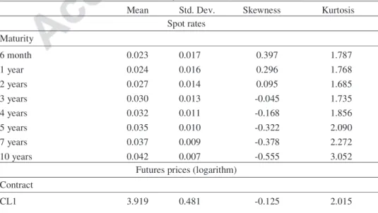
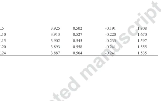
Table 1 displays some descriptive statistics for spot rates for each maturity and for the (log) futures prices for different contract maturities. Spot rates are characterized by a positive and decreasing skewness up to 2 years which, for longer maturities, is negative and increasing in absolute values. The kurtosis lies below 3 (except for 10 years, 3.052). The mean of futures prices is around
30
$49-50, while the volatility is high and increases with the maturity of the futures contracts. The skewness is negative and increases, in absolute values, with the contracts. The kurtosis is less than 3, and is positive and decreasing. Thus, as expected, spot rates and oil futures prices seem not to be normally distributed.
[Insert Table 1 about here]
5.2 Estimation procedure
As there is a unique interest rate, we divide the estimation procedure in two parts. The parameters of the short rate are first estimated and then those of the spot price and the convenience yield. Whatever the state variable, we use the Kalman filter in conjunction with the maximum likelihood method.
The dynamic model can be cast in state space form and then we employ the Kalman filter to estimate the parameters of the model and the time series of the unobservable state variables (see, for instance, [67]). Among the first authors to adopt this method, there are, for instance, Pennacchi [68] and Babbs and Nowman [69] for the term structure estimation, and Schwartz [11] for commodities. The discrete-time Kalman filter is an estimation methodology for recursively calculating optimal estimates of unobserved state variables given the information provided by noisy observations. A measurement equation relates the observed variables – on the one hand, spot rates, and, on the other
31
hand futures prices- to unobserved state variables. The discrete time version of the stochastic process followed by the latter – on the one hand, the short rate, and, on the other hand, the (log)spot commodity price and the convenience yield – is described by the transition equation.
The zero coupon yields can be written:
t T T t C t r t T T t D t T T t LnB T t R B B B B B B B − − − = − − = (, ) (, ) () (, ) ) , ( αˆ
with initial condition R(0,TB).
The measurement and the transition equations are then:
t Bi Bi Bi Bi Bi t T T t C t r t T T t D T t R α +υ − − − = (, ) () (, ) ) , ( ˆ for i = 1, ..., N and t = 1, ..., NT B
(
)
t t t t r e e t r ϑ α α ω + − + − = −∆ −∆ ) 1 ( 1 ) (where ωt and υt are (N,1)-dimensional vectors of serially uncorrelated disturbances such that
(
)
(
σ α)
ω α 2 / 1 , 0 2 2 t r t N e ∆ − − and υt N(0,Ω).From the expressions of the futures price, the (log)spot price and the convenience yield, the measurement and transition equations are as follows:
[
Hi Hi]
[
k Hi]
t Hi t t X T t D t r T t D T t K T t LnH υ δ α ~ ) ( ) ( ) , ( 1 ) ( ) , ( ) , ( ) , ( = + ˆ + − ˆ +32
(
kt)
kt t S S S t t X e t t e t t r t t X ω δ δ σ λ σ δ ~ ) 1 ( ) 1 ( 0 1 ) 1 ( 2 1 ) ( ) ( 2 + − − ∆ − ∆ + − ∆ − + − = −∆ ∆ −for i = 1, ..., N and t = 1, ..., NTB, where ωt
~ and
t
υ~ are (N,1)-dimensional vector of serially
uncorrelated disturbances such that:
(
)
(
−)
(
−)
− ∆ − ∆ − ∆ − k e k e k e N kt kt S S t k S S S t 2 / 1 2 / 1 2 / 1 , 0 ~ 2 2 2 2 2 δ δ δ δ δ σ σ σ ρ σ σ ρ σ ω and ) ~ , 0 ( ~ N Ω t υ .The estimation of model parameters is obtained by maximizing the log-likelihood function of innovations.
5.3 Estimation Results
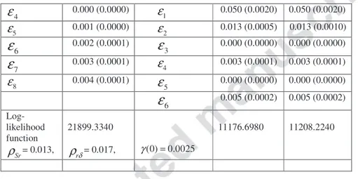
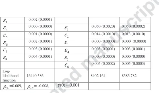
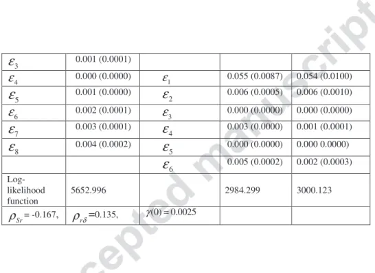
Tables 2, 3 and 4 show the parameter estimates, with their respective standard errors given in parentheses, of the short rate, the spot price, and the convenience yield, the estimated standard deviations of the measurement errors, , and the log-likelihood value, for the Schwartz 3-factor model and the incomplete information model. Our objective is to study the stability of the parameters estimates and to compare the two models with regard to their ability to fit the observed data by using the RMSE criterion, widely employed in the relevant literature. The RMSE is used since it measures
33
the squared errors between the model price (Schwartz’s or incomplete information) and the market price. It indicates how close the model is fitted to the data points. For the stability of the parameter values we consider three different panel-data: Panel A for the whole period (2001-2010, 522 weekly observations), panel B from 2001 to 14 July 2008 (391 weekly observations), panel C from 15 July 2008 to 2010 (131 weekly observations). To examine the performance of the models, we split the data into an in-sample set from 2001 to 2009 and an out-of-sample set for 2010. The first serves to estimate the models and to derive parameters values, while the latter will be used to test the out-of-sample performance of the models. As mentioned in the description of the data, the in-sample set is a period with high fluctuations characterized by an increase, a decrease then an increase again in oil prices. It is a sufficiently long period with a non monotonic evolution over time in oil prices. It is therefore an appropriate period for parameters estimation. For the incomplete information model, in order to obtain the initial value, γ , of the estimation error, we calculate the annualized monthly convenience yields (see [12]) for different maturities and for different dates and then we compute the variance of these convenience yields.
[Insert Table 2 about here]
As can be seen in these tables, all the parameters are statistically significant. Whatever the period, the speed parameters as well as k are positive and highly significant, which suggests that both the short rate and the convenience yield follow a mean-reverting process. However, these
34
parameters are not stable across panels, but the two models give similar values for k. The volatilities of the spot price and the convenience yield are stable over time except for σS for panel C and the two
models give close values for these volatilities. λS not only varies significantly from one period to
another (as λδ), but the two models result in different values for λS because this price of risk plays a
distinct role in the two models.
[Insert Table 3 about here]
The correlation coefficient between the spot price and the convenience yield is high and positive. Indeed, the convenience yield and the spot price are related through inventory decisions (e.g. [52]). During periods of low inventories, the probability that shortages will occur is greater, and hence the spot price as well as the convenience yield should be high. Conversely, when inventories are abundant, the spot price and the convenience yield tend to be low. The correlation between the interest rates, and spot prices and the convenience yield are low. In particular, ρSr although positive for panel
A, is negative for panels B and C in accordance with [51] and [54] who have argued that high real interest rates reduce commodity prices, and vice-versa.
[Insert Table 4 about here]
The performance of the models is assessed by using the RMSE criterion between model and observed market prices. Figures 2, 3 and 4 depict the RMSE for each contract maturity for the two models and for different periods: from 2001 to 2010, from 2001 to 2009 (in-sample) and for 2010
35
(out- of-sample). A simple inspection of these figures reveals that the best results are obtained for intermediate maturities, while the worst results are derived for the shortest maturities and, albeit to a lesser extent, for the longest maturities whatever the model. A comparison of the two models shows that the incomplete information model behaves better than the Schwartz model in the case of the whole period and for in-sample. The out-of-sample RMSE of Schwartz’s model is lower than that of the incomplete information model for short maturities, while is greater for longer maturities.
[Insert Figures 2, 3 and 4 about here]
The estimated parameters are used to compute option prices for the two models. Prices for short-term (three months, i.e. Tc = 3 months) options, as well as for longer-term (twelve months)
options are calculated. For all these options, the underlying deliverable asset is assumed to be a commodity futures contract with a maturity of six months. Prices are also calculated relative to the option “moneyness”. Exercise prices are selected so that K = H(T) for « at-the-money » (ATM) options, while « out-of-the-money » (OTM) and « in-the-money » (ITM) mean, respectively, H(T) = 0.9K and H(T) = 1.1K.
[Insert Table 5 about here]
Whatever the option maturity, Schwartz’s model prices are higher than those of the incomplete information model (except for some rare cases). Table 5 displays the average price difference between the two models for different options maturities and for different moneyness. The higher the options
36
maturity, the higher the difference between the two models’ prices. Moreover, this difference becomes more important when futures prices increase. The most important spread is obtained in July 2008 when futures prices reached a peak. The moneyness has a relative small effect on this spread, although it gets its higher value for OTM options.
6. Concluding Remarks
In order to account for the unobservable character of the instantaneous convenience yield, this paper investigates, in a valuation model, how the estimated convenience yield, conditional on the information provided by the spot commodity price and the instantaneous interest rate, can affect forward and option on forward prices, as well as their futures counterparts. A three-factor incomplete information model is developed which encompasses the two-factor and one-factor models. Unlike other incomplete information models, closed form solutions are derived for forward and futures prices, and for option values. These analytical solutions highlight especially the fact that the initial values of the estimate of the convenience yield and of the estimation error respectively have a strong effect on commodity derivatives prices. An empirical study suggests that our model, in terms of the RMSE
37
criterion, provides, in general, better results than Schwartz’s (1997) three-factor model for futures prices. Moreover, the latter results in higher prices for options.
The economic framework of this paper can be extended in several directions. First, a continuous time economy can be considered populated by two types of agents with heterogeneous beliefs (Detemple and Murthy, [70]). Second, some important observed and empirically detected characteristics of commodities, such as seasonality and jumps, may be included in our framework. Third, future research might allow convenience yields to be functions of prices and interest rates, as it seems to be in the case in the real world, rather than being an exogenous shock13. Finally, it would be interesting to examine how transactions costs modify our model and how impact derivatives prices14.
Acknowledgments
Constantin Mellios and Anh Lai, gratefully acknowledge research funding from the Laboratory of Excellence (Labex) « Financial Regulation ».
Appendix A: The inference problem
There are n observable processes, Y(t), described by a system of SDEs:
13 We thank a referee by suggesting us this extension of our model.
14
38
(
())
( ( )) () )) ( ( ) ( * 1 0 A t dt I Y t dz t A t Y I t dY Y Y σ θ + + = (A.1)with initial condition Y(0). I(Y(t)) is (n, n) diagonal matrix,
A
0and
A
1 are (n,1) vectors andσ
Y is a (n, n) matrix of constants. (t) is a n-dimensional unobservable state variable following the stochastic process:(
())
( ) ) ( * 1 0 a t dt dz t a t dθ = + θ +σθ θ (A.2)with initial condition (0).
a
0and
a
1 are (n, 1) vectors of constants andθ
σ
is a (n, n) matrix of constants. *( )and *( ) t z tzY θ are n-dimensional imperfectly correlated Wiener processes.
(0) is assumed to be normally distributed with mean m(0) and variance (0). This initial distribution and the structure of the stochastic processes of Y(t) and (t) imply that the distribution of
(t) conditional on the information, at time t, provided by Y(t), FY
(t), is (conditionally) Gaussian. The conditional mean and the estimation error are given respectively by: m(t) E
(
(t)FY(t))
θ = and
(
)(
)
(
() () () ()' ())
) (t =E θ t −mt θ t −mt FY t γ .A direct application of Theorem 12.1 in Liptser and Shiryayev [58] (see also [18]) results in the following expressions for m(t), (t) and the innovation process:
(
())
(
())
() ) ( ' 1 1 1 0 amt dt t A dzt a t dm γ YσY − Σ + Ω + + = ,(
) (
)
[
a t t a t A t A]
dt t d Y ' ' 1 ' 1 ' 1 1 () ( ) () () ) ( γ γ γ γ γ = Σθ + + − Ω+ Σ Ω+ ,39
(
)
[
I Y t dY t A Amt dt]
t dz() Y ( ( )) () 0 1 () 1 1 + − = − − σ , where , and ' 3 ' 2 ' 1σ Y σYρσY σ ρσY ρ σθ θ θ θ = Σ = Ω=Σ . ρi ,i=1,2,3are correlation matrices.
In the case of this paper, there are two correlated observable processes, S(t) and r(t), whose dynamics are given by equations (1) and (2) and one unobservable state variable, (t), obeying SDE (3). Equations (A.1) and (A.2) can be rewritten:
+ − + − = ) ( ) ( 0 0 ) ( 0 1 )) ( ( 1 0 0 ) ( ) ( ) ( * * t dz t dz dt t t r t S t dr t dS r S S r S σ σ δ β α µ ,
(
())
() ) ( * t dz dt t k t dδ = δ −δ +σδ δ ,with initial conditions S ,randδ.
(
)
(
)
. 0 0 ' δ δ δ δ δ δ δ σ ρ σ σ ρ σ σ σ ρ ρ σ r S r S r S r S = = Ω , Σθ ≡Σδ =σδ2 and = = Σ 2 2 ' 0 0 1 1 0 0 r Sr Sr S Sr Sr Y r S r S r S r S σ σ σ ρ σ σ ρ σ σ σ ρ ρ σ σ .The processes satisfied by m(t) and (t) (with initial conditions m and ) are then: