Extending Rate Monotonic Analysis with Exact Cost of Preemptions for Hard Real-Time Systems

HAL Id: inria-00413487

https://hal.inria.fr/inria-00413487

Submitted on 4 Sep 2009

HAL is a multi-disciplinary open access

archive for the deposit and dissemination of

sci-entific research documents, whether they are

pub-lished or not. The documents may come from

teaching and research institutions in France or

abroad, or from public or private research centers.

L’archive ouverte pluridisciplinaire HAL, est

destinée au dépôt et à la diffusion de documents

scientifiques de niveau recherche, publiés ou non,

émanant des établissements d’enseignement et de

recherche français ou étrangers, des laboratoires

publics ou privés.

Extending Rate Monotonic Analysis with Exact Cost of

Preemptions for Hard Real-Time Systems

Patrick Meumeu Yomsi, Yves Sorel

To cite this version:

Patrick Meumeu Yomsi, Yves Sorel. Extending Rate Monotonic Analysis with Exact Cost of

Preemp-tions for Hard Real-Time Systems. Proceedings of 19th Euromicro Conference on Real-Time Systems,

ECRTS’07, 2007, Pisa, Italy. �inria-00413487�

Extending Rate Monotonic Analysis with Exact Cost of Preemptions for Hard

Real-Time Systems

Patrick MEUMEU YOMSI

INRIA Rocquencourt

Domaine de Voluceau BP 105

78153 Le Chesnay Cedex - France

Email: patrick.meumeu@inria.fr

Yves SOREL

INRIA Rocquencourt

Domaine de Voluceau BP 105

78153 Le Chesnay Cedex - France

Email: yves.sorel@inria.fr

Abstract

In this paper we study hard real-time systems com-posed of independent periodic preemptive tasks where we assume that tasks are scheduled by using Liu & Layland’s pioneering model following the Rate Monotonic Analy-sis (RMA). For such systems, the designer must guaran-tee that all the deadlines of all the tasks are met, other-wise dramatic consequences occur. Certainly, guarantee-ing deadlines is not always achievable because the pre-emption is approximated when using this analysis, and this approximation may lead to a wrong real-time exe-cution whereas the schedulability analysis concluded that the system was schedulable. To cope with this problem the designer usually allows margins which are difficult to assess, and thus in any case lead to a waste of resources. This paper makes multiple contributions. First, we show that, when considering the cost of the preemption during the analysis, the critical instant doesnot occur upon

si-multaneous release of all tasks. Second, we provide a technique which counts the exact number of preemptions of each instance for all the tasks of a given system. Fi-nally, we present an RMA extension which takes into ac-count the exact cost due to preemption in the schedulabil-ity analysis rather than an approximation, thus yielding a new and stronger schedulability condition which elimi-nates the waste of resources since margins are not neces-sary.

1 Introduction

This paper deals with the problem of executing hard real-time systems found in the domains of automobiles, air traffic control, process control, telecommunications, etc, on a single processor. Such systems often consist of independent periodic preemptive tasks that must meet their deadlines in order to avoid the occurrence of dra-matic consequences [1, 2]. Certainly, guaranteeing dead-lines cannot always be achieved because the scheduling of the tasks is based on the assumption that the cost of the

preemption is approximated within the worst case execu-tion time (WCET) of tasks [3, 4, 5]. In fact, this approx-imation may be wrong because it is difficult to count the exact number of preemptions of each instance for a given task even though the costα of one preemption is easy to know for a given processor. Actually, this costα repre-sents the context switching time that the processor needs when a preemption occurs. The context switch includes the storage of the context as well as the restoration of the context. Since we are interested in embedded systems we only consider predictable processors without a cache or complex internal architecture (e.g. ARM2, etc.) [6, 7]. Therefore, this approximation may lead to a wrong real-time execution whereas the schedulability analysis con-cluded that the system was schedulable. To cope with this problem the designer usually allows margins which are difficult to assess, and which in any case lead to a waste of resources since the worst case response time is larger than the WCET when an instance of a task has been pre-empted [8, 9]. Note that the worst-case response time of a task is the longest time it takes, among all instances of that task, to execute each instance from its release time [10]. There have been very few studies addressing this is-sue of counting the exact number of preemptions. Among them, the most relevant ones are the following. A. Burns, K. Tindell and A. Wellings in [11] presented an analysis that enables the global cost due to preemptions to be fac-tored into the standard equations for calculating the worst case response time of any task, but they achieved that by considering the maximum number of preemptions instead of the exact number. Juan Echag¨ue, I. Ripoll and A. Cre-spo also tried to solve the problem of the exact number of preemptions in [12] by constructing the schedule using idle times and counting the number of preemptions. But, they did not really determine the execution overhead in-curred by the system due to these preemptions. Indeed, they did not take into account the cost of each preemption during the analysis. Hence, this amounts to considering only the minimum number of preemptions because some preemptions are not considered: those due to the increase in the execution time of the task because of the cost of

preemptions themselves.

In this paper, we first show that the critical instant [3] does not occur when all tasks are released simultaneously if we consider the cost of the preemption during the anal-ysis. Second, we propose a new scheduling algorithm which counts the exact number of preemptions of each instance for all tasks. Finally, we propose a new and stronger schedulability condition than Liu & Layland’s condition, which takes into account the exact cost due to preemption in the schedulability analysis. This new condi-tion always guarantees a correct execucondi-tion and eliminates any waste of resources since no margins are necessary.

We assume that tasks are scheduled by using Liu & Layland’s pioneering model according to Rate Monotonic Analysis (RMA) [3, 13]. That is to say, we are in the fixed priority context and the highest fixed priority is assigned to the task with the shortest period [14, 15]. When two tasks have the same period they are scheduled arbitrarily [16]. We consider a set of n independent periodic preemp-tive tasksτi,1 ≤ i ≤ n. Each taskτiis an infinite sequence

of instances1_τk

i,k ∈ N+, and is characterized by a WCET Ci, not including the approximation of the cost of the

pre-emption, a period Ti, and a release time relative to 0, ri.

This means that instances corresponding to taskτiare

re-leased at times ri+kTi, k ≥ 0. The instance released at

time ri+kTihas ri+ (k + 1)Tias its deadline, i.e. the

re-lease time of the next instance. We re-index tasks in such a way that T1≤T2≤ · · · ≤Tn. Consequently,τireceives

priority i2_{and we assume that tasks are ready to run at}

their release times (idle time is forbidden in the presence of ready tasks).

For the sake of readability and without any loss of gen-erality, from now on, although it is not realistic, we con-sider the cost of one preemption for the processor to be α = 1 time unit in all the examples. This high cost of pre-emptions in terms of the execution time of tasks is used to illustrate the impact of not accounting for preemptions correctly.

In addition, it is worth noticing that the analysis per-formed here would work even if the preemption cost is not a constant.

The remainder of this paper is structured as follows: section 2 gives a counterexample on the critical instant when the cost of preemption is considered. Section 3 de-scribes the model and gives the notations used through-out the paper. Section 4 provides the definitions we need to take into account the exact cost of preemption in the schedulability analysis presented in section 5. That sec-tion explains in detail, on the one hand, our scheduling algorithm which counts the exact number of preemptions and, on the other hand, derives the new schedulability con-dition. The complexity of our algorithm is discussed in section 6. We conclude and propose future work in sec-tion 7.

1_{Throughout the paper all subscripts refer to tasks whereas all}

super-scripts refer to instances.

2_{1 represents the highest priority.}

2 Critical instant

The critical instant when the cost of the preemption is approximated within the WCET of tasks is such that the release time of the first instance of tasks occurs simultane-ously [3], that is to say ri=0 for all 1 ≤ i ≤ n. However,

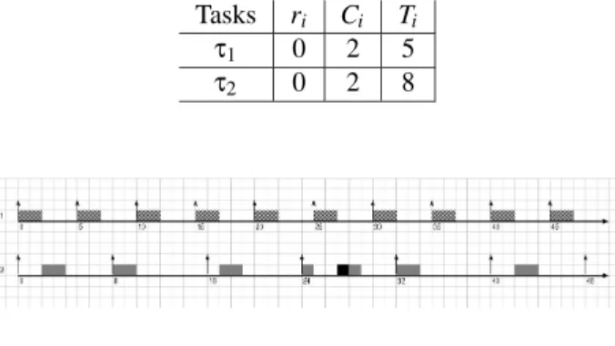
this is not necessarily the critical instant when the cost of preemptions is considered, see the counterexample de-picted in figure 1 (the “¥” represents the preemption cost).

Tasks ri Ci Ti

τ1 0 2 5

τ2 0 2 8

Figure 1. Schedule under RMA with the cost of preemption considered, ri=0

In figure 1 the response time (4 time units) of taskτ2

in its first instance (corresponding to the critical instant) is shorter than the response time (5 time units) of its fourth instance. This is becauseτ2 has been preempted in the

fourth instance and then, the cost of the preemption has been added to the WCET without any approximation, and used to compute the response time in that instance.

If the first instances of all tasks are released simultane-ously, then this is repeated every hyperperiod H, thus as stated in [3, 1] it is sufficient to perform the schedulability analysis in the interval [0,H]. H is the least common mul-tiple of the periods of the tasks: H = lcm{T1,T2,· · · ,Tn}.

For this reason, in this paper, we assume that all tasks are released simultaneously. Since the worst case response time of a task may not occur in the first instance (see figure 1), we consider all instances of a task within a hyperpe-riod, and perform the schedulability analysis only within the first hyperperiod.

Because we intend to take into account the exact cost of the preemption, and because all tasks, except the first one, may be preempted, the proposed technique gives a schedulability condition for each task individually accord-ing to tasks with higher priority. Our schedulaccord-ing algorithm calculates the exact number of preemptions per instance of every task. This individual analysis leads, at the end, to a schedulability condition for all the tasks.

3 Model and Notations

Throughout this paper, all timing characteristics in our model are assumed to be non-negative integers, i.e. they

are multiples of some elementary time interval (for ex-ample the “CPU tick”, the smallest indivisible CPU time unit).

Since all tasks except the one with the highest priority may be preempted, the execution time of a task may vary from one instance to another. We call preempted execution time (PET) the WCET augmented with the exact cost due to preemptions for each instance of a task within a hyper-period. Thus, the PET denoted Ck

i for instanceτki of task

τiis greater than or equal to its WCET Ci. It depends on

the instance and on the number of preemptions occuring in that instance. Its calculation will be detailed below.

The following model (depicted in figure 2) is an exten-sion, with the exact cost of preemption, of the classical model [3] for systems of tasks executed on a single pro-cessor.

Figure 2. Model

τi= (Ci,Ti): A task

Ti: Period ofτi

Ci: WCET ofτinot including the preemption

approximation, Ci≤Ti

α: Temporal cost of one preemption for a given processor τk

i: The kthinstance ofτi

Np(τki): Exact number of preemptions ofτiinτki

Ck

i =Ci+Np(τki) ·α: PET of τiwith its preemption cost

inτk i rk i = (k − 1)Ti: Release time ofτki Rk i: Response time ofτki

Ri: Worst-case response time ofτi

From the point of view of task τi, since it may

only be preempted by higher priority tasks, we define the hyperperiod at level i, Hi, which is given by Hi =

lcm{Tj}τj∈hep(τi), where hep(τi)is the set of tasks with

a priority higher than or equal to taskτi. Hence, taskτi

is releasedσitimes in each hyperperiod at level i starting

from 0, with

σi=Hi

Ti =

lcm{Tj}τj∈hep(τi)

Ti (1)

The total utilization factor is usually given by Un= n

∑

i=1 Ci Ti (2)

Recall that in (2) Cidoes not include the approximation

of the cost of the preemption for taskτi. If Un>1 then the

task set is not schedulable with any algorithm [17]. Thus, a set of n tasks may be schedulable if and only if Un≤1

[18, 19]. Indeed, Uncan be lower than or equal to 1 and

the system not schedulable.

According to the number of preemptions Np(τki)of task

τi= (Ci,Ti)in each instanceτki, its PET Cki may be

dif-ferent from one instance to another, except for the task with the highest priorityτ1which can never be preempted.

However, because taskτi may only be preempted by the

set of tasks with a priority higher thanτi denoted hp(τi)

3_{, then there are exactlyσidifferent PETs for taskτi. In}

other words, from the point of view of any taskτi, 1 ≤ i ≤ n, there exists a functionπ : N+_{× N}+_{−→ N}+σi_× N+, defined asπ(C_i,Ti) =π(τi) = ((Ci1,C_i2,· · · ,Cσ_ii),Ti),

which maps the WCET Ciof taskτiinto its respective PET

Ck

i in each instanceτki. Therefore, each taskτi= (Ci,Ti)

has an imageτ0

i=¡(Ci1,C_i2,· · · ,Cσ_ii),Ti¢. Consequently,

we define the exact total utilization factor to be U∗ n= n

∑

i=1 1 σi Ã_σ i

∑

k=1 Ck i Ti ! =Un+ n

∑

i=1 1 σi Ã_σ i

∑

k=1 Np(τki) ·α Ti ! (3) Remark that ifα = 0, then equation (3) reduces to the classical total utilization factor Unwhen the global cost

due to preemption is approximated within the WCET of tasks. Therefore, the global cost due to preemptions in-curred by the system is

εn= n

∑

i=1 1 σi Ã_σ i

∑

k=1 Np(τki) ·α Ti ! (4) Now we have to calculate Np(τki)for all k = 1,··· ,σiand

for all i = 1,··· ,n. To do so, let us recall some useful algebra that we need to achieve this goal.

4 Definitions

For a given set of n tasks, we define the exact total utilization factor at level j, 1 ≤ j ≤ n to be

U∗ j = j

∑

i=1 1 σi Ã_σ i

∑

k=1 Ck i Ti ! =Uj+ j

∑

i=1 1 σi Ã_σ i

∑

k=1 Np(τki) ·α Ti ! (5) It is worth noticing that since we are in a fixed prior-ity context, and thus we carry out the schedule from the highest priority task towards lower priority tasks, then to every instanceτk

i of a task τi= (Ci,Ti)is associated an

ordered set of Ti time units where some are already

ex-ecuted because of the execution of a higher priority task, and the others are still available for the execution of taskτi

in that instance. We call this ordered set which describes the state of each instance τk

i a Ti-mesoid. We denote a

time unit already executed by an “e” and a time unit still available by an “a”. Obviously, the switch from an a to an e represents a preemption if the WCET of the task un-der consiun-deration is strictly greater than the cardinal of the

sub-set corresponding to the first sequence of a. Accord-ing to the remainAccord-ing execution time this situation may oc-cur again. For example, {e,e,e,a,a,a,e,e,a,a,e,a,a} is a mesoid where the first 3 time units have already been ex-ecuted, the next 3 time units are available, followed again by 2 already executed, then 2 available followed by one already executed and which ends with 2 available. For the sake of clarity and without any loss of generality, we call a sub-set corresponding to a sequence of consecutive time units already executed a consumption, and we rep-resent it by its cardinal inside brackets (c), with c ∈ N+_.

In addition, we enumerate the sequence of available time units according to the natural numbers. This enumeration is done from the end of the first sequence of time units already executed in that instance. Each of these natural numbers corresponds to the number of available time units since the end of the first consumption. They represent all the possible PETs of the task under consideration in the corresponding instance. Each of these natural numbers is called an availability. Thus, the previous 13-mesoid can be re-writen as: {(3),1,2,3,(2),4,5,(1),6,7}. It has three consumptions 3, 2, 1, and seven availabilities 1, 2, 3, 4, 5, 6, 7. If the PET of the task under consideration is equal to 6 then there are two preemptions. Notice that the sum of all the consumptions of a mesoid and the high-est availability in that mesoid, is equal to the period of the task under consideration. From the point of view of task τi= (Ci,Ti), there are as many Ti-mesoids as instances in

the hyperperiod Hi at level i, because task τi may only

be preempted by tasks in hp(τi). Therefore, there are

σi Ti-mesoids in Hi which will form a sequence of Ti

-mesoids. We call

L

b i = n

M

ib,1,

M

_ib,2,· · · ,

M

_ib,σi o the se-quence ofσiTi-mesoidsbefore τiis scheduled. For

exam-ple,

L

b

i = {{(5),1,2,3,(2),4},{1,2,(3),3,4,(3),5}} is a

sequence ofσi=2 11-mesoids. The process for building

the sequence

L

b

i of taskτiwill be detailed later on in this

paper.

Still, from the point of view of taskτi, we define for

each mesoid

M

b,k

i ,1 ≤ k ≤σiof the sequence

L

ibthe

cor-responding universe Xk

i of τi to be the set which

con-sists of all the availabilities of

M

b,k

i . That is to say,

all the possible values that Ck

i can take in

M

ib,k.

Re-call that Ck

i denotes the PET ofτi inτki, the kth instance

of τi. For the previous example of a sequence of

11-mesoids,

M

ib,2= {1,2,(3),3,4,(3),5}, and thus we have

X2

i = {1,2,3,4,5}.

Taskτiwill be said to be potentially schedulable if and

only if      U∗ i−1+C_Ti i ≤1 Ci∈Xik ∀k ∈ {1,··· ,σi} (6) The first equation of (6) verifies that the minimum exact total utilization factor at level i is less than or equal to 1. Indeed, U∗

i−1+C_Ti i ≤U

∗

i because all WCET

Ci ≤ Cik,∀k ≥ 1, and when taskτiis shedulable Ui∗≤1

must hold. Theσiother equations verify that Ci belongs

to all the universes.

Since Ci∈ {1,2,··· ,Ti}, ∀1 ≤ i ≤ n, let us define the

following binary relation on each instance

R

: “WCET Cγ1 leads to the same number of preemptions

as WCET Cγ2”, Cγ1,Cγ2∈ {1,2,··· ,Ti}

R

is clearly an equivalence relation on {1,2,··· ,Ti}

(reflexive, symmetric, transitive). Now, since Xk i ⊆

{1,2,··· ,Ti}, ∀1 ≤ k ≤σi, thus

R

is also an equivalence

relation on Xk

i,∀1 ≤ k ≤σiand each Xik,k = 1,··· ,σi

to-gether with

R

is a setoid 4_{. From now on, we consider}

only the restriction of

R

on Xk

i,k = 1,··· ,σibecause Xik

represents all the available time units in instanceτk i.

The equivalence classes of each universe are the sub-sets of availabilities determined by two consecutive con-sumptions in the associated mesoid. In the remainder of this paper, we call these equivalence classes the cells of the universe. Hence, for the above example, we have

X1

i: [0]1= {1,2,3} and [1]1= {4}

X2

i: [0]2= {1,2} and [1]2= {3,4} and [2]2= {5}

where for m ∈ N and 1 ≤ k ≤σi, [m]kdenotes the subset

of Xk

i composed of the availabilities which are preempted

m times. Thus, for the previous example,

L

b

i can also be written as

L

b i = {{(5), [0]1 z }| { 1,2,3,(2), [1]1 z}|{ 4 },{ [0]2 z}|{ 1,2 ,(3), [1]2 z}|{ 3,4 ,(3), [2]2 z}|{ 5 }} This means for taskτithat its PET Cik∈Xik, i.e. in its kth

instance, k = 1,2, should not exceed 4 in the first instance, and 5 in the second instance otherwise taskτicannot be

schedulable. We call

L

a i = n

M

ia,1,

M

_ia,2,· · · ,

M

_ia,σi o the sequence ofσiTi-mesoids of taskτiafter τiis scheduled.

L

a

i is a function of

L

ibwhich itself is a function of

L

i−1a ,

both detailed as follows. We build the sequence

L

b

i for taskτi by using an

in-dex ζ which enumerate, according to natural numbers, the time units in the sequence

L

a

i−1 of task τi−1 after

τi−1 is scheduled. This enumeration is done whether

the time units have already been consumed or are still available. ζ starts from the first time unit of the first mesoid

M

a,1

i−1towards the last time unit of the last mesoid

M

a,σi−1

i−1 , and then circles around to the beginning of the

first mesoid

M

a,1

i−1 again. This process of counting is

thuscyclic. Each time ζ = Ti, a Ti-mesoid is obtained

for the sequence

L

b

i and then the next Ti-mesoid is

ob-tained by starting to count again from the next time unit to the current one. This process is repeated until we get theσi Ti-mesoids of

L

ib. Since taskτ1 is the

high-est priority task, hep(τ1) = {τ1} and thusσ1=H_T1 1 =1

thanks to equation (1). Moreover, because it is never pre-empted, we have

L

b 1 = n

M

1b,1 o = {{1,2,··· ,T1}} and

L

a 1= n

M

a,1 1 o = {{(C1),1,2,··· ,T1−C1}}. The sequence

L

a

i is deduced from the sequence

L

ib

be-cause all the available time units will have been consumed up to the response time (detailed later on) within each mesoid

M

b,k

i ,k = 1,··· ,σiof taskτiafter τiis scheduled.

Notice that the response time in each mesoid depends on π for task τi.

To summarize, for every taskτi, we have

τi:       

L

b i = n

M

b,1 i ,

M

_ib,2,· · · ,

M

_ib,σi o

L

a i = n

M

a,1 i ,

M

ia,2,· · · ,

M

ia,σi o Both

L

b

i and

L

iaconsist of a finite numberσiof Ti-mesoids

in each sequence.

5 The proposed approach

In this section we outline our approach that leads to a new and stronger schedulability condition than the condi-tion proposed by Liu & Layland [3], Joseph and Pandya [20], Lehoczky et al. [5], Audsley et al.[21], etc. in the sense that it takes the cost of preemption accurately into account in the schedulability analysis rather than using an approximation. The intuitive idea behind our approach uses a system of arithmetic for integers, where numbers “wrap around” after they have reached a certain value: the period of the task under consideration. In other words, our approach uses a modulo T arithmetic where T is the period of a task.

5.1 Scheduling of two tasks

Let us motivate the general result of our approach by considering the simple case of the scheduling problem of two tasks τ1= (C1,T1)andτ2= (C2,T2), with T1≤T2.

Under RMA,τ1is assigned the higher priority. This latter

statement implies thatbefore τ1is scheduled, its WCET C1can potentially take any value from 1 up to the value of

its period T1, therefore

L

1b=

n

M

1b,1

o

= {{1,2,··· ,T1}}.

Since taskτ1is never preempted, thus Ck₁=C1,∀k ≥ 1 andσ1=1 andτ01=π(τ1) = ((C1),T1). In addition, its

re-sponse time is also equal to C1. Hence,after τ1is

sched-uled, it has consumed C1 time units, and thus there

re-main T1−C1availabilities in each of its instances.

Conse-quently, the corresponding T1-mesoids associated to task

τ1are given by τ1:       

L

b 1= n

M

1b,1 o = {{1,2,··· ,T1}}

L

a 1= n

M

1a,1 o = {{(C1),1,2,··· ,T1−C1}}

Now, the challenge is to schedule taskτ2by taking into

account the exact cost of preemptions. Thanks to

every-thing we have presented up to now, the construction of

L

b

2 consists ofσ2=H_T2

2 T2-mesoids. Furthermore, the

se-quence

L

b

2 is built by using the indexζ and enumerating cyclically the time units in the sequence

L

a

1. The

con-struction of

L

b

2is based on the intuitive idea of a modulo

T2arithmetic. After the construction of

L

₂b, we can

eas-ily determine the corresponding universe Xk

2 to each T2

-mesoid

M

b,k

2 , k = 1,··· ,σ2. Thus, thanks to equation (6),

taskτ2is potentially schedulable if and only if

     U∗ 1+C_T2 2 ≤1 C2∈X₂k ∀k ∈ {1,··· ,σ2} (7)

We give the following example in order to illustrate these conditions. Let us consider a set of two tasks τ1

andτ2with T1=6, T2=8, and C1=2, C2=3. We have

τ1:   

L

b 1= {

M

1b,1} = {{1,2,3,4,5,6}}

L

a 1= {

M

1a,1} = {{(2),1,2,3,4}} Sinceσ2=H2 T2 =3, thus we derive

L

b 2 which consists of

a sequence of three 8-mesoids by using the indexζ as ex-plained in the previous section on the sequence

L

a

1. We obtain

L

b 2 = n

M

b,1 2 ,

M

2b,2,

M

2b,3 o = {{(2),1,2,3,4,(2)},{1,2,3,4,(2),5,6}, {1,2,(2),3,4,5,6}}

For each 8-mesoid

M

b,k

2 ,1 ≤ k ≤ 3, composing

L

2b, we

build the corresponding universe Xk

2,1 ≤ k ≤ 3. These

universes are given by τ2: ° ° ° ° ° ° X1 2= {1,2,3,4} X2 2= {1,2,3,4,5,6} X3 2= {1,2,3,4,5,6}

From these universes, we deduce that taskτ2is

poten-tially schedulable because for each resulting universe Xk

2, we have      U∗ 1+C_T2 2 = 2 6+ 3 8 ≤1 3 ∈ Xk 2 ∀k ∈ {1,··· ,σ2}

Now, thanks to the equivalence relation

R

on each Xk

2

for k = 1,··· ,3, the cells of each universe are given by for universe X1 2: [0]1= {1,2,3,4} for universe X2 2: [0]2= {1,2,3,4} and [1]2= {5,6} for universe X3 2: [0]3= {1,2} and [1]3= {3,4,5,6}

where for m ∈ N and 1 ≤ k ≤σ2, [m]kdenotes the subset

of Xk

2 composed of the availabilities which are preempted

m times. Thus, for this example,

L

b

2can also be written as

L

b 2 = {{(2), [0]1 z }| { 1,2,3,4,(2)},{ [0]2 z }| { 1,2,3,4,(2), [1]2 z}|{ 5,6 }, { [0]3 z}|{ 1,2 ,(2), [1]3 z }| { 3,4,5,6}}

Here we have all we need to calculate the exact number of preemptions Np(τk2)and then the corresponding PET C2k

of taskτ2in its kthinstance, 1 ≤ k ≤σ2.

Since taskτ2 is potentially schedulable (equation (7)

holds), thus, its WCET C2 belongs to one and only one

cell [θ1]kin each universe X2k,k = 1,··· ,σ2(see figure 4

when i = 2) since each (Xk

2,

R

)is a setoid. As such, the PET Ck

2 is different from the actual value of the WCET

C2 in the associated mesoid as soon as taskτ2 must be

preempted at least once. This occurs when C2∈X2k\[0]k

for any k with 1 ≤ k ≤σ2, (see figure 5 when i = 2).

In each universe Xk

2,1 ≤ k ≤σ2, the number of

preemp-tions Np(τk₂)and the PET Ck₂of taskτ2are computed by

using the following algorithm. Initialization:                  C₂k,1=C2 Bk,1_=C2 qk,1_=θ 1 Ak,1₌θ

∑

1−1 m=0 card([m]k) rk,1=C2k,1−Ak,1 For l ≥ 1, we compute Bk,l+1= l

∑

j=1 Ak, j+ (rk,l+θl·α) (8)

By using the same idea as for a fixed-point algorithm, this computation stops as soon as either two consecutive val-ues of Bk, j_{,j ≥ 1, belong to the same cell or there exists}

µ1≥1 such that Bk,µ1 >card(X₂k). Figure 6 when i = 2 illustrates the same idea as for a fixed point algorithm. In this latter case, taskτ2is not schedulable because the

pe-riod (deadline) of the task is thus exceeded. Actually, if Bk,l+1_≤card(Xk

2), then ∃θl+1≥0 such that

Bk,l+1∈ [θ1+ · · · +θl+1]k

Ifθl+1=0 then Bk,l+1 and Bk,l belong to the same cell,

therefore expression (9) holds with µ2=l + 1 and Np(τk2)

is given by (10), else ifθl+16=0, then we compute

             Ck,l+1₂ =rk,l+θl·α qk,l+1_=θ l+1 Ak,l+1₌θ1+···+θ

∑

l+1−1 m=θ1+···+θl card([m]k) rk,l+1=Ck,l+1−Ak,l+1

and thus we derive the next value of Bk, j_{. The algorithm}

is stopped as soon as ∃µ2≥1 such that θµ2=0 (9) and therefore Np(τk2) = µ2−1

∑

j=1 qk, j ₍₁₀₎

Thanks to equation (10), for each k = 1,··· ,σ2, we

com-pute the PET Ck

2of taskτ2in X2k, i.e. in its kthinstance,

including its exact preemption cost. Figure 6 when i = 2, in addition to illustrate the same idea as for a fixed point algorithm, also shows the PET of the taskτi in instance

τk i.

C2k=C2+Np(τk2) ·α (11)

Consequently, the image ofτ2by functionπ is given by

τ0

2=π(τ2) =¡(C21,C2₂,· · · ,C₂σ2),Ti¢ (12)

The response time Rk

2,1 ≤ k ≤σ2of taskτ2in its kth

instance, i.e. in the kth _T

2-mesoid is obtained by

sum-ming Ck

2with all the consumptions appearing before C2kin

the corresponding mesoid. Once this has been done, the worst-case response time R2of taskτ2is given by

R2=max{1≤k≤σ2}(Rk2)

The sequence

L

a

2 is deduced from sequence

L

2bby

up-dating the latter since all time units up to the response time have now been consumed in every mesoid. Hence, by us-ing expression (3), the exact total utilization factor of the CPU is given by U∗ 2= 2

∑

i=1 1 σi Ã_σ i

∑

k=1 Ck i Ti ! =U2+_σ1 2 Ã_σ 2

∑

k=1 Np(τk2) ·α T2 ! (13) Let us illustrate this result on the previous example. We still assumeα = 1 to be the cost of one preemption for the processor in order to give a clear indication of the impact of the preemption. We recall that C2=3, taskτ2is

potentially schedulable, and

L

b 2 = {{(2), [0]1 z }| { 1,2,3,4,(2)},{ [0]2 z }| { 1,2,3,4,(2), [1]2 z}|{ 5,6 }, { [0]3 z}|{ 1,2 ,(2), [1]3 z }| { 3,4,5,6}}

In both the first and second universes, C2∈ [0]k,k = 1,2; thus C1

2 =C22=C2 whereas in the third universe,

C2∈ [1]3. The computation of Np(τ32)is summarized in

the following table.

From the second column of table 1, we get Np(τ32) =1

and thus we obtain C3

2=3+1·1 = 4. Hence, the image of

taskτ2by functionπ is given by τ02=π(τ2) = ((3,3,4),8).

Therefore, U∗ 2 = 2 6 + 1 3 µ 3 + 3 + 4 8 ¶ =0.750 whereas

Table 1. computation of Np(τ3₂)

Steps q3,l _C3,l

2 A3,l r3,l B3,l

1 1 3 2 1 4

2 0 2 2 0 4

U2= 2₆+3₈ =0.708. The response times of taskτ2 in

each mesoid thanks to our previous definition are given by

R1

2=3 + 2 = 5, R22=3, and R32=4 + 2 = 6

Hence, from this approach we can obviously deduce the worst-case response time R2of taskτ2: R2=6. Task

τ2is schedulable and its response time Rk2,1 ≤ k ≤σ2in

its kth _{instance, i.e. in the k}th_T

2-mesoid, is the first

con-sumption in

M

a,k

2 of sequence

L

2a. Figure 3 depicts the

schedule of this example taking into account the exact cost of preemtion.

For more than two tasks notice that

L

a

2is deduced from

L

b

2by updating the latter as follows.

L

b 2 = {{(2), [0]1 z }| { 1,2,3,4,(2)},{ [0]2 z }| { 1,2,3,4,(2), [1]2 z}|{ 5,6 }, { [0]3 z}|{ 1,2 ,(2), [1]3 z }| { 3,4,5,6}} ®¶ O²

O²O²O²

L

a

2= {{(5),1,(2)},{(3),1,(2),2,3},{(6),1,2}}

Figure 3. Execution of two tasks following RMA with exact cost of preemption

5.2 Scheduling of n > 2 tasks

The strategy that we will adopt in this section to calcu-late both the exact number of preemptions and the PETs of a given task in each of its instances is the generaliza-tion to a system of n > 2 tasks of everything we have pre-sented in the previous section for the simple case of two tasks. Indeed, the basic idea behind this approach con-sists, for each task, in filling availabilities in each mesoid with slices (cardinal of cells) of its PET which takes into account the cost of the exact number of preemptions nec-essary for its schedule. Recall that at each preemption oc-curence,α time units add to the remaining execution time of the instance of the task under consideration.

Before going through our proposed algorithm, we re-call the exact total utilization factor at level j, U∗

j, with 1 ≤ j < n, U∗ j = j

∑

i=1 1 σi Ã_σ i

∑

k=1 Ck i Ti ! =Uj+ j

∑

i=1 1 σi Ã_σ i

∑

k=1 Np(τki) ·α Ti ! (14) Without any loss of generality, we assume that all tasks have different periods, that is to say Ti<Tj for 1 ≤ i <

j ≤ n. A sub-system of tasks {τi= (Ci,Ti)}1≤i≤p, with

1 ≤ p < n, is said to be maximal when the the exact total utilization factor at level p is smaller than or equal to 1, and the exact total utilization factor at level (p + 1)th is strictly larger than 1, this occurs when

U∗

p≤1 and Up+1∗ >1 (15) This means that the sub-system {τi= (Ci,Ti)}1≤i≤pis

the largest sub-system schedulable on the processor ac-cording to RMA.

5.3 Scheduling algorithm

We assume that the first i − 1 tasks with 2 ≤ i ≤ n have already been scheduled, and that we are about to schedule the ith _{task, i.e. taskτ}

i, which is potentially schedulable,

i.e. _     U∗ i−1+C_Ti i <1 Ci∈Xik ∀k ∈ {1,··· ,σi}

As in the previous section for the construction of

L

b

2

using index ζ on the sequence

L

a

1, the sequence

L

ib of

taskτiis built thanks to indexζ on the sequence

L

i−1a of

taskτi−1. The sequence

L

ibconsists ofσiTi-mesoids

M

ib,k

with k = 1,··· ,σisince taskτimay only be preempted by

tasks belonging to hp(τi). Therefore, we can determine

the universes Xk

i ∀k ∈ {1,··· ,σi} when the sequence

L

a

i−1 is known. Again, the response time Rki,1 ≤ k ≤σi

of taskτiin its kthinstance, i.e. in the kth Ti-mesoid will

be obtained by summing Ck

i with all consumptions prior to

Ck

i in the corresponding mesoid. The worst-case response

time Riof taskτiwill be given by

Ri=max{1≤k≤σi}(Rki)

This equation leads us to say that taskτiwill be

schedu-lable if and only if

Ri≤Ti (16)

Again,

L

a

i will be deduced from

L

ibby updating the

latter since all time units up to the response time will have been consumed in each mesoid. For the sake of clarity, note that when updating

L

b

i, whenever there are two

con-secutive consumptions in the same mesoid, this amounts to considering only one consumption which is the sum of the previous consumptions. That is to say that after de-termining the response time of taskτi in its kth mesoid,

if

M

a,k

M

a,k

i = {(c1+c2),1,2,···} without any loss of

general-ity.

Below, we present our scheduling algorithm which, for a given task on the one hand, counts the exact number of preemptions in each of its instances, and on the other hand, provides its PET in each of its instances in order to take the cost of the preemption into account accurately in the schedulability condition. It has the twelve following steps. Since the highest priority task, namely taskτ1, is

never preempted, the loop starts from the index of the sec-ond highest priority task, namely taskτ2as we carry out

the schedule towards lower priority tasks.

1: for i = 2 to n do

2: Compute the number σi of times that task τi =

(Ci,Ti)is released in the hyperperiod at level i

σi=H_Ti i =

lcm{Tj}τj∈hep(τi)

Ti

Recall that Hi=lcm{T1,T2,· · · ,Ti}

3: Build the sequence

L

_ibof Ti-mesoids of taskτi

be-fore it is scheduled. This construction consists of σiTi-mesoids

M

_ib,kwith k = 1,··· ,σi, and is based

on a modulo Tiarithmetic using the the indexζ on

the sequence

L

a i−1.

4: For each Ti-mesoid

M

ib,k resulting from the

pre-vious step, build the corresponding universe Xk i

which is composed of the set of all availabilities in

M

b,k

i . Notice that this set corresponds to the set

of all possible values that the PET Ck

i of taskτican

take in

M

b,k i .

5: Build all the cells for each universe X_ik. A cell of

Xk

i is composed of the subset of availabilities

de-termined by two consecutive consumptions in the associated mesoid

M

b,k

i .

6: Compute both the exact number of preemptions

and the PET Ck

i of taskτiin each universe Xik,1 ≤ k ≤σi, resulting from the previous step thanks to

the algorithm inlined in this step. This algorithm is necessary because, sinceτiis potentially

schedu-lable, i.e. its WCET Ci belongs to one and only

one cell [θ1]kin each universe Xik(see figure 4), we

must verify that it is actually schedulable.

Figure 4. task τipotentially schedulable

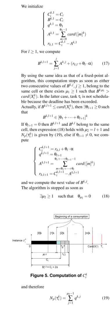
We initialize                  C_ik,1=Ci Bk,1_=C i qk,1_=θ1 Ak,1₌θ

∑

1−1 m=0 card([m]k) rk,1=Ck,1i −Ak,1 For l ≥ 1, we compute Bk,l+1₌

_∑

l j=1 Ak, j_{+ (r} k,l+θl·α) (17)

By using the same idea as that of a fixed-point al-gorithm, this computation stops as soon as either two consecutive values of Bk, j_{,j ≥ 1, belong to the}

same cell or there exists µ1≥1 such that Bk,µ1 > card(Xk

i). In the latter case, taskτiis not

schedula-ble because the deadline has been exceeded. Actually, if Bk,l+1_≤card(Xk

i), then ∃θl+1≥0 such

that

Bk,l+1∈ [θ1+ · · · +θl+1]k

Ifθl+1=0 then Bk,l+1and Bk,l belong to the same

cell, then expression (18) holds with µ2=l + 1 and

Np(τki)is given by (19), else ifθl+16=0, we

com-pute              C_ik,l+1=rk,l+θl·α qk,l+1_=θ l+1 Ak,l+1₌θ1+···+θ

∑

l+1−1 m=θ1+···+θl card([m]k) rk,l+1=Cik,l+1−Ak,l+1

and we compute the next value of Bk, j_.

The algorithm is stopped as soon as

∃µ2≥1 such that θµ2 =0 (18) Figure 5. Computation of Ck i and therefore Np(τki) = µ2−1

∑

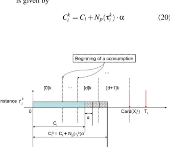
j=1 qk, j (19)

For each k = 1,··· ,σi, the PET Cki of taskτiin Xik

is given by Ck

i =Ci+Np(τki) ·α (20)

Figure 6. PET of task τiin instance τki: Cik

7: Deduce the image τ0_i = π(τi) =

(¡C1

i,C2_i,· · · ,C_iσi¢,Ti)of taskτiresulting from the

previous step.

8: Determine the response time Rk

i,1 ≤ k ≤σiof task

τiin its kthinstance, i.e. in the kthTi-mesoid. This is

obtained by summing Ck

i and all the consumptions

prior to Ck

i in the corresponding mesoid. Deduce

the worst-case response time Riof taskτi.

Ri=max{1≤k≤σi}(Rki)

It is worth noticing that taskτiis schedulable if and

only if

Ri≤Ti.

9: Build the sequence

L

_ia by updating all the Ti

-mesoids of the sequence

L

b i.

10: Compute the exact total utilization load factor at level i. That is to say

U∗ i = i

∑

j=1 1 σj Ã_σj

∑

k=1 Ck j Tj ! =Ui+ i

∑

j=1 1 σj Ã_σj

∑

k=1 Np(τkj) ·α Tj ! .

11: If U_i∗≤1 then increment i, and go back to step 2 as long as there remain potentially schedulable tasks in the system.

12: If U∗

i > 1, then the sub-system {τj =

(Cj,Tj)}1≤ j≤i−1 was already maximal. In

this case, the system {τi = (Ci,Ti)}1≤i≤n is not

schedulable.

13: end for

Thanks to the above algorithm, a necessary and suf-ficient schedulability condition for a system of n tasks

{τi= (Ci,Ti)}1≤i≤n, all released at the same time and

scheduled according to RMA, which takes the cost due to preemption accurately into account is given by U∗ n= n

∑

i=1 1 σi Ã_σ i

∑

k=1 Ck i Ti ! =Un+ n

∑

i=1 1 σi Ã_σ i

∑

k=1 Np(τki) ·α Ti ! ≤1 (21) Example

Still with the same assumption thatα = 1 let us con-sider {τ1,τ2,τ3,τ4}to be a system of four tasks with the

characteristics defined in table 2.

Table 2. Characteristics of example 4

Ci Ti

τ1 2 6

τ2 3 10

τ3 2 15

τ4 3 30

According to RMA, the lower the index of a task is, the higher its priority is. Thus, as depicted in table 2,τ1

has the highest priority and taskτ4has the lowest priority.

Thanks to our scheduling algorithm, σ1=1, thus for taskτ1

τ1:                   

L

b 1= n

M

b,1 1 o = {{ [0]1 z }| { 1,2,3,4,5,6}} τ1= (2,6) 7−→τ01= ((2),6)

L

a 1= n

M

a,1 1 o = {{(2),1,2,3,4}} σ2=3, thus for taskτ2

τ2:                                                   

L

b 2 = n

M

b,1 2 ,

M

₂b,2,

M

₂b,3 o = {{(2), [0]1 z }| { 1,2,3,4,(2), [1]1 z}|{ 5,6 }, { [0]2 z}|{ 1,2 ,(2), [1]2 z }| { 3,4,5,6,(2)}, { [0]3 z }| { 1,2,3,4,(2), [1]3 z }| { 5,6,7,8}} τ2= (3,10) 7−→ τ02= ((3,4,3),6)

L

a 2 = n

M

2a,1,

M

₂a,2,

M

₂a,3 o

= {{(5), 1, (2), 2, 3}, {(6), 1, 2, (2)}, {(3), 1, (2), 2, 3, 4, 5}}

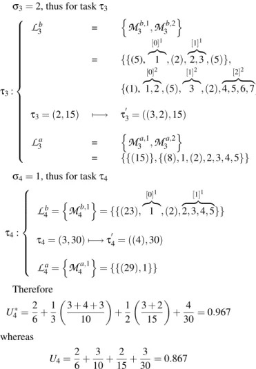
σ3=2, thus for taskτ3 τ3:                                     

L

b 3 = n

M

3b,1,

M

₃b,2 o = {{(5), [0]1 z}|{ 1 ,(2), [1]1 z}|{ 2,3 ,(5)}, {(1), [0]2 z}|{ 1,2 ,(5), [1]2 z}|{ 3 ,(2), [2]2 z }| { 4,5,6,7}} τ3= (2,15) 7−→ τ03= ((3,2),15)

L

a 3 = n

M

a,1 3 ,

M

₃a,2 o = {{(15)},{(8),1,(2),2,3,4,5}} σ4=1, thus for taskτ4

τ4:                   

L

b 4= n

M

b,1 4 o = {{(23), [0]1 z}|{ 1 ,(2), [1]1 z }| { 2,3,4,5}} τ4= (3,30) 7−→τ04= ((4),30)

L

a 4= n

M

a,1 4 o = {{(29),1}} Therefore U∗ 4=2₆+1₃µ 3 + 4 + 3₁₀ ¶ +1 2 µ 3 + 2 15 ¶ + 4 30=0.967 whereas U4=2 6+ 3 10+ 2 15+ 3 30=0.867

The schedule of this task set following RMA with the cost of preemption considered is depicted in figure 7.

Figure 7. Execution of a task set by follow-ing RMA and considerfollow-ing the exact cost of preemption

whereas the schedule of the same set of tasks following RMA without the cost of preemption is depicted in figure 8.

6 Complexity of the proposed scheduling

al-gorithm

For every task, the schedulability analysis is performed only once. In this analysis we walk through the iteration

Figure 8. Execution of a task set by follow-ing RMA with the cost of preemption ap-proximated

space in order to calculate the number and positions of available time units. Hence, the time and space complex-ity for every task is

O

(m0), where m0 is the number of

time units in the sequence of mesoids of each task. To calculate the PET of a taskτiwhich includes the

ex-act cost of preemption within a given instanceτk

i, the

com-plexity of our algorithm is

O

¡σi·σhp·m0¢, where σiis the

number of instances of the current task in a hyperperiod at level i, andσhp=

i−1

∑

j=1

σj is the number of higher priority

instances in a hyperperiod at level i. This complexity is explained as follows. Our analysis is a per instance anal-ysis, and hence includes the factorσifor every task. For

each instance, we need to calculate the exact number of preemptions and the PET which includes the exact cost of these preemptions. To calculate the exact number of preemptions, we need to partition every instance. Since the number of potential preemption occurences is equal to the number of higher priority instances within the hyper-period at level i, the factorσhpis included. Although the

complexity of the calculation of a PET adds a factor m0

to the complexity, it is actually a small number since the range of available time units or availabilities between two consecutive consumptions is limited by the largest one. However, it is worth noticing that when the periods of the tasks form an harmonic sequence, the time and space com-plexity of our algorithm is

O

(n), where n is the number of tasks in the task set.

7 Conclusion and future work

This paper makes three main contributions. First, we give a counterexample on the critical instant when the cost of preemption is considered. Second, we present a tech-nique which counts the exact number of preemptions for every intance of the task under consideration in a given task set. Finally, we provide an RMA extension which takes into account the exact cost due to preemption in the schedulability analysis rather than using an approxima-tion. This technique provides a new and stronger schedu-labily condition since no margins are necessary.

Further-more, this new condition always guarantees a correct exe-cution of the system and eliminates the waste of resources. Future work will study the case where the deadline of a task is smaller than its period.

References

[1] Joseph Y.-T. Leung and M. L. Merrill. A note on preemptive scheduling of periodic, real-time tasks. Information Processing Letters, 1980.

[2] Ray Obenza and Geoff. Mendal. Guaranteeing real time performance using rma. The Embedded Systems Conference, San Jose, CA, 1998.

[3] C.L. Liu and J.W. Layland. Scheduling algorithms for multiprogramming in a hard-real-time environ-ment. Journal of the ACM, 1973.

[4] Lehoczky-J.P. Sha, L. and R. Rajkumar. Solutions for some practical problems in prioritized preemp-tive scheduling. Proceedings of the IEEE Real-Time Systems Symposium, 1986.

[5] J.P. Lehoczky, L. Sha, and Y Ding. The rate mono-tonic sheduling algorithm: exact characterization and average case bahavior. Proceedings of the IEEE Real-Time Systems Symposium, 1989.

[6] Lichen Zhang. Predictable architecture for real-time systems. International Conference on Information, Communications and Signal Processing, 1997. [7] Engblom-J. Berg, C. and R. Wilhelm. Perspective

workshop: Design of systems with predictable be-haviour. Dagstuhl Seminars, 2004.

[8] H. Chetto and M. Chetto. On the acceptation of non-periodic time critical tasks in distributed sys-tems. Proc. 7th IFAC Workshop Distributed Com-puter Control Systems (DCCP-86), 1986.

[9] H. Chetto and M. Chetto. Some results on the ear-liest deadline scheduling algorithm. IEEE Transac-tions on Software Engineering, 1989.

[10] H. Chetto, Silly M., and Bouchentouf T. Dynamic scheduling of real-time tasks under precedence con-traints. The Journal of Real-Time Systems, 1990. [11] Tindell K. Burns A. and Wellings A. Effective

anal-ysis for engineering real-time fixed priority sched-ulers. IEEE Trans. Software Eng., 1995.

[12] I. Ripoll J. Echage and A. Crespo. Hard real-time preemptively scheduling with high context switch cost. In Proceedings of the 7th Euromicro Workshop on Real-Time Systems, 1995.

[13] Klein Mark H. Sha, Lui and John B. Goode-nough. Rate monotonic analysis. Technical Report CMU/SEI-91-TR-6 ESD-91-TR-6, 1991.

[14] Tei-Wei Kuo Jian-Jia Chen. Procrastination for leakage-aware rate-monotonic scheduling on a dy-namic voltage scaling processor. LCTES’06, Ot-tawa, Ontario, Canada, 2006.

[15] Buttazzo G. Bini, E. A hyperbolic bound for the rate monotonic algorithm. IEEE Proc. of the 13th Euromicro Conf. on Real-Time Systems, pp. 59-66, 2001.

[16] J. Goossens and Richard P. Overview of real-time scheduling problems. Euro Workshop on Project Management and Scheduling, Invited Paper, 2004. [17] Giorgio C. Buttazzo. Rate monotonic vs edf:

Judge-ment day. Real-Time Systems, vol. 29, Number 1, pp. 5-26, 2005.

[18] Mok A.K. Chen, D. and T. Kuo. Utilization bound revisited. IEEE Transactions on computer, Vol. 52, No. 3, pp. 351-361, 2003.

[19] Natarajan S. Park, D.W. and A. Kanevsky. Fixed pri-ority scheduling of real-time systems using utization bounds. Journal of Systems and Software, Elsevier. Vol. 33, pp.57-63, 1996.

[20] M. Joseph and P. Pandya. Finding response times in real-time system. BCS Computer Journal, 1986. [21] N.C. Audsley, A. Burns, M.F. Richardson, Tindell

K., and A.J. Wellings. Applying new scheduling the-ory to static priority pre-emptive scheduling. Soft-ware Engineerung Journal, 1993.