Présentée et soutenue le 10/05/2016 par : Florian SIMATOS

MANUSCRIT MANUSCRIT

Présenté pour l’obtention de

L’HABILITATION À DIRIGER DES RECHERCHES

Délivrée par : l’Université Toulouse 3 Paul Sabatier

Présentée et soutenue le 10/05/2016 par : Florian SIMATOS

Théorèmes limite fonctionnels, processus de branchement et réseaux stochastiques

Functional limit theorems, branching processes and stochastic networks

Patrick CATTIAUX Professeur des universités JURY Président du jury Jean-François DELMAS Professeur des universités Membre du jury Thomas DUQUESNE Professeur des universités Rapporteur Sergey FOSS Full professor Membre du jury David GAMARNIK Full professor Rapporteur Laurent MICLO Directeur de recherche Membre du jury

École doctorale et spécialité :

MITT : Domaine Mathématiques : Mathématiques appliquées Unité de Recherche :

ISAE-SUPAERO Directeur de Thèse :

Laurent MICLO Rapporteurs :

Maury BRAMSON , Thomas DUQUESNE et David GAMARNIK

This work is licensed under a Creative Commons

Attribution-NonCommercial-NoDerivatives 4.0 International License.

Acknowledgements

First and foremost, I would like to thank Professor Maury Bramson, Professor Thomas Duquesne and Professor David Gamarnik for accepting to review my manuscript.

Some of their papers rank among the most influential in the fields of branching pro- cesses and stochastic networks, and it is an honor to have them as reviewers.

I would also like to thank Professor Laurent Miclo for accepting to act as direc- tor of my habilitation, as well as Professor Patrick Cattiaux, Professor Jean-François Delmas and Professor Sergey Foss for being part of my defense committee. I am learning on a daily basis how scarce a resource time is and it makes me even more thankful for the time everybody has devoted to my project.

Research is a weird business: it is done 90% alone, but these are the 10% re- maining, made of lively discussions and interactions, which make it so exciting. It is therefore my sincere pleasure to thank here my various co-authors as well some colleagues who have played an important role in my career at some point even though it did not translate into a publication: the work presented here was only possible thanks to them. My warmest thanks thus go to Elie Aïdekon, François Bac- celli, Vincent Bansaye, Sem Borst, Niek Bouman, Ed Coffman, A. Ganesh, Fabrice Guillemin, Tom Kurtz, Peter Lakner, Amaury Lambert, Marc Lelarge, Lasse Leskëla, Sarah Lilienthal, D. Manjunath, Alexandre Proutière, Josh Reed, Philippe Robert, Emmanuel Schertzer, Shuzo Tarumi, Danielle Tibi, Johan van Leeuwaarden, Remco van der Hofstad, Gil Zussman and Bert Zwart. I hope to have the chance – and, more importantly, the time – to pursue our rewarding collaborations.

The four-year period that I have spent in the Netherlands between CWI and TU/e represents the most exciting time I have had from a scientific standpoint. Although the previous list only contains a few Dutch names, I would also like to address a general thank to my formeer Dutch colleagues who have made these four years so enjoyable and productive: most of the work presented here has indeed been carried out while in the Netherlands. I would like to thank more specifically Bert Zwart, Sem Borst and Johan van Leeuwaarden for funding my post-doctoral positions.

My special thanks to Odile Riteau, our enthusiastic secretary at ISAE-SUPAERO, for her precious help in arranging all the practical details of the defense.

Finally, the writing of this manuscript has come at a turning point of my career and personal life: I was hired at ISAE-SUPAERO three months earlier and Gaëtan was barely two-month old. My habilitation and lecture notes being now written, I do not anticipate any more acknowledgements in the near future and so I seize this opportunity to thank one more time Sandrine for her love and support – may it last forever.

iii

Contents

Acknowledgements iii

Summary vii

1 Introduction 1

1.1 Functional law of large numbers and central limit theorem . . . . 1

1.2 Motivation . . . . 3

1.3 Notation used throughout the document . . . . 6

2 Two theoretical results on weak convergence 11 2.1 Introduction . . . . 11

2.2 A sufficient condition for tightness . . . . 14

2.3 Weak convergence of regenerative processes . . . . 17

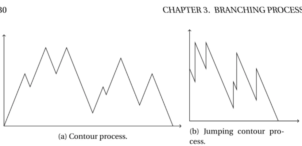
3 Branching processes 23 3.1 Introduction . . . . 24

3.2 Galton–Watson processes in varying environments . . . . 30

3.3 Binary, homogeneous Crump–Mode–Jagers processes . . . . 37

3.4 Crump–Mode–Jagers trees with short edges . . . . 45

4 Stochastic networks 53 4.1 Introduction . . . . 53

4.2 Processor-Sharing queue length process . . . . 56

4.3 A stochastic network with mobile customers . . . . 64

4.4 Lingering effect for queue-based scheduling algorithms . . . . 72

5 Branching processes in mathematical finance 81 5.1 Study of a model of limit order book . . . . 81

6 Research perspectives 91 6.1 Branching processes . . . . 91

6.2 Stochastic averaging via functional analysis . . . . 93

6.3 Stochastic networks . . . . 94

v

Summary

Overview

This manuscript describes some of the work I have been doing since 2010 and the end of my PhD. As the title suggests, it contains three main parts.

Functional limit theorems: Chapter 2 presents two theoretical results on the weak convergence of stochastic processes: one – Theorems 2.2.1 and 2.2.2 – is a suf- ficient condition for the tightness of a sequence of stochastic processes and the other – Theorem 2.3.1 – provides a sufficient condition for the weak convergence of a sequence of regenerative processes;

Branching processes: in Chapter 3, scaling limits of three particular types of branch- ing processes are discussed: 1) Galton–Watson processes in varying environments, 2) binary and homogeneous Crump–Mode–Jagers processes and 3) Crump–Mode–

Jagers processes with short edges;

Stochastic networks: Chapter 4 presents three results on stochastic networks: 1) scaling limits of the M/G/1 Processor-Sharing queue length process, 2) study of a model of stochastic network with mobile customers and 3) heavy traffic delay performance of queue-based scheduling algorithms.

These topics are closely intertwined: tightness of Galton–Watson processes in varying environments studied in Section 3.2 is obtained thanks to Theorem 2.2.1 of Chapter 2; results of Section 4.2 on the Processor-Sharing queue are essentially ob- tained by combining results on binary and homogeneous Crump–Mode–Jagers pro- cesses from Section 3.3 together with the sufficient condition for the convergence of regenerative processes from Chapter 2; and scaling limits of the model of mo- bile network of Section 4.3 rely on the same theoretical result. In order to give an overview of how these results relate to each other, Chapters 2, 3 and 4 are briefly presented next.

Chapter 5 is devoted to the study of a model of limit order books in mathematical finance: the main technical tool is a coupling with a branching random walk, and it also adopts an excursion point-of-view similar in spirit as in Section 2.3 whereby the limiting process is characterized by its excursion measure.

Finally, the manuscript is concluded in Chapter 6 with research perspectives.

vii

Summary of Chapter 2

Section 2.2 presents the main result of [BS, BKS], namely a sufficient condition for the tightness of a sequence of stochastic processes (X

) of the form

E ^{h 1} ∧ d(X

(t), X

(t ))

| X

(u ), u ≤ s i

≤ F

(t) − F

(s), n ≥ 1, 0 ≤ s ≤ t, with d the distance, β > 0 and (F

) a sequence of càdlàg functions with F

J₁

→ F in the Skorohod J

topology. This result extends a result from Kurtz [74] where F was assumed to be continuous: allowing general càdlàg F was motivated by the study of processes in varying environments that may exhibit accumulation of fixed points of discontinuity. This criterion is used in Section 3.2 to prove the tightness of a se- quence of Galton–Watson processes in varying environments.

Section 2.3 presents the main results of [LS14]. This paper establishes a new method for proving the weak convergence of a sequence of regenerative processes from the convergence of their excursions. It is shown that for a tight sequence (X

) of regen- erative processes to converge, it is enough that the first excursion with “size” > ε converges together with its left- and right-endpoints and its size. Here the size of an excursion is given by a general measurable mapping ϕ with values in [0, ∞ ]. This approach was motivated by the study of the Processor-Sharing queue in Section 4.2 and also proved useful to study a stochastic network with mobile users discussed in Section 4.3.

Summary of Chapter 3

Section 3.2 presents results on scaling limits of Galton–Watson processes in vary- ing environments obtained in [BS15]. These results adopt the original approach of Grimvall [44] via the study of Laplace exponents and extend results of Kurtz [75] and Borovkov [17] by allowing offspring distributions to have infinite variance. The price to pay is a loss of generality in the drift term, corresponding to the first moments of the offspring distributions, which is assumed to have finite variation.

Section 3.3 presents results on scaling limits of binary and homogeneous Crump–

Mode–Jagers processes obtained in [LSZ13, LS15]. The main tool is the connec- tion with Lévy processes, whereby a binary and homogeneous Crump–Mode–Jagers process is seen as the local time process of a compound Poisson process with drift stopped upon hitting 0. Assuming that the sequence of Lévy processes converges, it is shown that this implies weak convergence of the sequence of associated local time processes – and thus of the binary and homogeneous Crump–Mode–Jagers processes – in the finite variance case where the limiting Lévy process is a Brow- nian motion. In the infinite variance case, this always implies convergence of the finite-dimensional distributions but extra assumptions are needed to get weak con- vergence.

Section 3.4 continues the study of Crump–Mode–Jagers processes and presents re- sults from [SS]. Results in the binary and homogeneous case suggest a general in- variance principle, namely that scaling limits of Crump–Mode–Jagers processes with

“short” edges, i.e., where individuals do not live for “long” periods of time, should

belong to the universality class of Galton–Watson processes. Results of this section

quantify and make rigorous this intuition by shifting the viewpoint from the branch- ing processes to the random chronological trees encoding them. In particular, the height and contour processes of such trees are studied and their scaling limits are derived under a “short” edge condition.

Summary of Chapter 4

Section 4.2 continues the presentation of results of [LSZ13]: here, the main object of study is the Processor-Sharing queue length process and the main tool, the Lamperti transformation which maps a binary, homogeneous Crump–Mode–Jagers process to an excursion of the queue length process of the M/G/1 Processor-Sharing queue. In particular, results of Section 3.3 together with continuity properties of the Lamperti transformation imply that “big” excursions of the Processor-Sharing queue length process converge. In view of the main result of Section 2.3, in order to get the con- vergence of the whole process, a control on the left- and right-endpoints and the size of excursions is needed, as well as tightness.

Section 4.3 presents results from [BS13, ST10] where a stochastic network with mo- bile users is studied. In this model, customers move within the network according to a Markovian dynamic independent from the service received, which is in sharp contrast with Jackson networks where movements are coupled with service com- pletion. This model is characterized by the coexistence of two time scales: a “fast”

time scale corresponding to the inner movements of customers and which acceler- ates as customers accumulate; and a “slow” time scale corresponding to arrivals to and departures from the network, which is bounded by the arrival and service rates and thus remains O(1). The coexistence of these two time scales induces new and original queueing phenomena which are studied in this section, in particular con- cerning stability and heavy traffic behavior. Moreover, scaling limits in the heavy traffic regime are established by invoking results of Section 2.3 for regenerative pro- cesses. In this context, a control of “big” excursions is achieved precisely because of the coexistence of these two time scales which imply a spatial state space collapse phenomenon when the network is overloaded.

Section 4.4 presents results from [SBB13] concerning the delay performance in heavy

traffic of queue-based algorithms. From a technical standpoint, this corresponds

to studying CSMA in the classical interference model, with the particular feature

that activation rates depend on the current workload through an activation ψ . Such

queue-based algorithms have received considerable attention in recent years, and it

is shown that a lingering effect lower bounds the delay performance which scales in

the heavy traffic regime ρ ↑ 1 at least as fast 1/(1 −ρ )

. Thus, these systems are prone

to inherent inefficiencies which proscribe achieving the optimal 1/(1 −ρ ) lower bound.

Chapter 1

Introduction

Contents

1.1 Functional law of large numbers and central limit theorem . . . . 1 1.2 Motivation . . . . 3 1.3 Notation used throughout the document . . . . 6

1.1 Functional law of large numbers and central limit theorem

Among the many important results from probability theory, two stand out promi- nently: the law of large numbers and the central limit theorem. Let throughout this introduction ( ξ

,k ∈ N ) be i.i.d. random variables and define the partial sums X (k ) = ξ

+· · ·+ξ

. Let

→ and →

denote almost sure convergence and convergence in distribution as n → ∞ , respectively.

Theorem 1.1.1 (Strong law of large numbers). If E ( |ξ

| ) < ∞ , then n

X (n)

→ E ( ξ

).

When E ( ξ

) 6= 0, the strong law of large numbers therefore justifies the approx- imation X (n) ≈ n E ( ξ

). If E ( ξ

) = 0 however, it only states that X (n) is negligible compared to n and leaves open the question of the right order of magnitude of X (n ) for large n: this question is, to some extent, settled by the central limit theorem.

Theorem 1.1.2 (Central limit theorem). Let N be a standard normal random vari- able: if, E ( ξ

) = 0 and E ( ξ

) = 1, then n

X (n) →

N .

Although presented here as the first order asymptotic expansion of X (n) in the critical case E ( ξ

) = 0, the central limit theorem can also be seen as the second or- der asymptotic expansion of X (n) in the non-critical case: indeed, Theorem 1.1.2 immediately entails that if ξ

has finite second moment, then n

(X(n) − n E ( ξ

)) converges in distribution to a normal random variable.

The problems considered in this manuscript deal with functional versions of these fundamental results. For the convergence of stochastic processes, we con- sider in this introduction the space of càdlàg functions endowed with the topology

1

of uniform convergence on compact sets (as limit processes will be almost surely continuous). In a functional setting, the strong law of large numbers takes the fol- lowing form.

Theorem 1.1.3 (Functional strong law of large numbers). For n ∈ N and t ∈ R

define X ¯

(t) = n

X ([nt ]): if E ( |ξ

| ) < ∞ , then X ¯

→ s with s(t) = t E ( ξ

).

Similarly as in the scalar case, this result does not provide the right order of mag- nitude of ¯ X

in the critical case E ( ξ

) = 0. A refined result is provided by the following functional central limit theorem. Throughout this manuscript, W refers to a stan- dard Brownian motion.

Theorem 1.1.4 (Functional central limit theorem). For n ∈ N and t ∈ R

define X ˆ

(t) = n

X ([nt ]): if E ( ξ

) = 0 and E ( ξ

) = 1, then X ˆ

→

W .

Similarly as in the scalar case, there are two ways to interpret the functional cen- tral limit theorem. On the one hand, it can be interpreted as saying that, in the critical case E ( ξ

) = 0, fluctuations of X ([nt ]) are of the order of n

:

(X ([nt ]),t ∈ R

) ≈ ¡

n

W (t), t ∈ R

¢ , E ( ξ

) = 0. (1.1) On the other hand, it can be seen as the second order asymptotic expansion of the process (X ([nt ]), t ∈ R

) as n → ∞ :

(X([nt ]) − ns(t), t ∈ R

) ≈ ¡

n

W (t), t ∈ R

¢ . (1.2)

Of course, these two viewpoints are equivalent, i.e., they lead to the same limit, but this is peculiar to the random walk case: in general, these two schemes will lead to different limits. This is for instance the case for the M /M/1 queue, and to see this let us begin by rewriting (1.1) in the following equivalent form:

¡ X ([n

t]),t ∈ R

¢ ≈ (nW (t), t ∈ R

) , E ( ξ

) = 0. (1.3) The interpretation of (1.1) is that one fixes the time-scale (n) and then looks for the correct order of magnitude of the fluctuations of X on this time-scale (n

):

this is actually the way we got to (1.1) in the first place. The interpretation for (1.3) reverses the viewpoint: one first fixes the space-scale (n) and then looks for the time-scale on which fluctuations are of this order (n

). Said otherwise, both (1.1) and (1.3) aim at going beyond the crude convergence ¯ X

→ 0 (the constant function with value 0) given by the functional strong law of large numbers, but they achieve this in different ways: (1.1) asserts that n

X ¯

(t ) →

W (t), which amounts to ampli- fying fluctuations of ¯ X

; whereas (1.3) asserts that ¯ X

(nt ) →

W (t), which amounts to speeding up ¯ X

.

Let us now illustrate the fact that (1.2) and (1.3) are not necessarily equivalent by considering the M/M/1 queue. Recall that an M/M/1 queue with arrival rate λ and service rate µ is the Markov process with generator

Ω (f )(k) = λ (f (k + 1) − f (k )) + µ 1 ^(k ≥ 1)( f (k − 1) − f (k )), k ∈ Z

, f : Z

→ R .

Let L

(t) be the number of customers in a critical M/M/1 queue at time t,

where the arrival and service rates λ , µ are equal and the superscript (n) refers to

the initial state: L

(0) = n . Note that this last relation fixes the scaling in space.

If ¯ L

(t) = n

L

(nt ), then the functional strong law of large numbers states that ¯ L

→ 1, the function which takes the constant value one, and there are now two kinds of central limit theorem. The first one deals with the second order asymptotics of ¯ L

, given by n

( ¯ L

− 1) →

(2 λ )

W : this is the analog of (1.2) for the M/M/1 queue. The second one amounts to scaling ¯ L

in time in order to get a more inter- esting limit: it states that ( ¯ L

(nt), t ∈ R

) → |

1 + (2 λ )

W | . This result is the ana- log of (1.1) and (1.3) for the M /M/1 queue, and thus indeed illustrates that (1.2) and (1.3) are not in general equivalent.

The problems considered in this manuscript belong to the second category: we will be interested in the scaling in time and space, without centering terms, of stochas- tic processes in the critical regime. The term scaling limits is a generic term which usually refers to such normalization schemes. Since one usually ends up with diffu- sion processes in the limit, it is also sometimes called diffusion approximation.

Mainly two classes of stochastic processes will be investigated: branching pro- cesses and stochastic networks. For branching processes, the critical regime cor- responds to the regime where the mean population size stays constant: it lies in- between the subcritical regime, where the mean population size decays exponen- tially fast, and the supercritical regime, where the mean population size increases exponentially fast.

For stochastic networks, the critical regime corresponds to the boundary of the stability region, defined as the set of parameters corresponding to a stable (e.g., pos- itive recurrent in the case of Markov processes) process. It is usually expressible in the form ρ = 1, with ρ the load of the network, and is referred to in the queueing literature as heavy traffic regime.

1.2 Motivation

The motivation for the large amount of literature dedicated to functional limit the- orems spans a wide range of reasons, both theoretical and applied.

Invariance principle

The deepest reason, in my view, takes its root in the so-called invariance principle.

This corresponds to the striking feature of Theorems 1.1.3 and 1.1.4 that the limits only depend on the distribution of X

through its first and (in the central limit the- orem setting) second moments. There are, of course, a wide variety of distributions with the same first and second moments but these differences are washed out in these asymptotic regimes. This principle has several profound implications.

From a theoretical standpoint, this makes it possible to classify processes ac-

cording to their scaling limits: we talk about universality class. For instance, when

looked through the suitable time-space lens, all finite variance random walks look

like a Brownian motion, a fuzzy statement made precise by Theorem 1.1.4. More

generally, the universality class of random walks is the class of Lévy processes, while

the universality class of branching processes is the class of continuous-state branch-

ing processes (CSBP). In contrast to random walks and branching processes, stochas-

tic networks do not form such a clear-cut class of stochastic processes, but as the

heavy traffic limit of Jackson networks and more generally of a broad class of open

queueing networks, semimartingale reflected Brownian motions probably stand out as the universality class of stochastic networks. Besides making it possible to clas- sify broad classes of stochastic processes, the fact that different processes have the same scaling limits make the latter play a prominent role in probability theory. For instance, the central role played by the Brownian motion in probability theory is to a large extent due to its prevalence in functional limit theorems: this generally jus- tifies the in-depth studies of these “universal” objects such as Lévy processes, CSBP and semimartingale reflected Brownian motions. In summary, invariance principles make it possible to reduce the dimensionality of the problem by putting forward a few canonical stochastic processes.

From an application standpoint, such invariance principles make it possible to identify the key parameters of the model under study. For instance, the fact that the semimartingale reflected Brownian motion arising as the heavy traffic approx- imation of open queueing networks only depends on the first two moments of the arrival and service distributions makes it possible to dimension such networks sim- ply based on these two parameters. In particular, one does not need to infer the whole distribution of these processes. Similarly, if one wishes to use Feller diffusion to model some particular population dynamic, one only needs to learn the first and second moments of the corresponding offspring distribution. Also, it must be noted that, although the critical case may appear as a very special case (indeed, it usually corresponds to a set of parameters of zero Lebesgue measure), it often turns out to be a relevant one in practice. For communication networks, an operator seeks to ensure finite delay while avoiding waisting capacity; for branching processes, the critical case can explain the long-time persistence of a population which in the sub- critical or supercritical cases would die out quickly or grow exponentially fast. These two simple examples illustrate the fact that there are often good “physical” reasons for a system to be in the critical regime.

Continuous mapping

Another motivation for establishing functional limit theorems comes from the strong notion of convergence considered. Indeed, we are considering convergence in dis- tribution of stochastic processes in the Skorohod J

topology: this is much stronger than, say, the notion of convergence of finite-dimensional distributions. One fun- damental advantage of this form of convergence is that it makes it possible to use of the continuous mapping theorem: if X

→

X , then φ (X

) →

φ (X ) for any func- tional φ almost surely continuous at X . For instance, in the real-valued case and if X is almost surely continuous, then the convergence X

→

X automatically implies the convergence sup

X

→

sup

X for any t ∈ R

, a conclusion which does not necessarily hold if X

merely converges to X in the sense of finite-dimensional dis- tributions. Thus once the convergence X

→

X is established, one gets for free the convergence of a vast number of other functionals of X

. This optimistic statement must nonetheless be tempered: in practice, it turns out (at least, in my experience) that most functionals φ of interest are not continuous, or that it is challenging to prove that they are almost continuous at the limit point.

Nevertheless, such an approach has proved immensely successful for proving functional limit theorems. For instance, as will be explained in Section 3.1.2, the convergence X

→ X with X

a random walk and X a Lévy process implies, by a di-

rect application of the continuous mapping theorem, the convergence of a sequence of Galton–Watson processes. Another typical application is to describe the dynamic of the pre-limit processes by stochastic differential equations, typically driven by Poisson processes, and use continuity arguments to show convergence toward a diffusion process which satisfies the corresponding limiting stochastic differential equations, typically driven by Brownian motions arising by compensating the pre- limit Poisson processes.

Besides, results of the kind φ (X

) →

φ (X ) are very useful for deriving approxima- tions because, in most cases, the limit process is more tractable than the pre-limit processes. First of all, there is a whole technical apparatus developed to study con- tinuous processes: when in the realm of the law of large numbers, the limits are usually described by ordinary differential equations for which an extensive theory is available; while when in the real of the functional central limit theorem, the theory of stochastic calculus makes it possible to perform explicit computation. Moreover, the limit processes are often by nature more tractable. For instance, although there is in general no tractable expression for the law of the supremum of a stochastic process on the time interval [0, t], for a Brownian motion we have

P µ

sup

0≤s≤t

W (s) ≥ x

¶

= r 2

π t Z

x

e

dy.

The functional convergence X

→

W combined with the continuous mapping theo- rem therefore justifies the approximation

P µ

sup

0≤s≤t

X

(s ) ≥ x

¶

≈ r 2

π t Z

x

e

dy.

Stationary distributions

Functional central limit theorems are concerned with the asymptotic behavior of processes over finite time intervals (at least, when considering the J

topology):

however, they can also turn out to be useful for studying stationary distributions.

In this case, one is faced with the problem of interchanging limits: starting from X

(t), if one first lets n → ∞ and then t → ∞ , one obtains the stationary distribu- tion of the scaling limit; while if one first lets t → ∞ and then n → ∞ , one obtains the asymptotic behavior of the stationary distribution of X

. Typically, directly studying the asymptotic behavior of the stationary distribution of X

can be a challenging task whereas, in part because scaling limits are usually more tractable than pre-limit processes, the stationary distribution of the scaling limit is a reasonable object. One thus would like to know when these two limits commute in order to gain insight into the asymptotic behavior of the stationary distributions associated to the sequence (X

). This approach has for instance been carried out to study the stationary dis- tribution of generalized Jackson networks in heavy traffic in [38], where the inter- change of limits was guaranteed by the existence of uniform geometric Lyapunov functions.

Fluid limits and stability of Markov processes

Last but not least, functional law of large numbers have gained in queueing theory a

tremendous impulse since the pioneering work of Rybko and Stolyar [103] and then

Dai [27], showing that the stability of a Markov process can be inferred from the sta- bility of the associated fluid model, see also the earlier work by Malyshev and Men- shikov [88]. In this setting, one is interested in determining whether some Markov process X is recurrent or not. The idea is to consider a sequence (x

) of initial states with k x

k → ∞ and to consider

X ¯

(t) = 1 k x

k X

¡

k x

k t ¢

where X

is the process started at X

(0) = x

. In many cases, the process ¯ X

will converge in distribution toward a deterministic function, called the fluid limit, and governed by a deterministic dynamical system, called fluid model. Rybko and Stol- yar then observed that stability of the original Markov process could be deduced from the stability of its fluid model, which opened the way to study the stability of more complex queueing systems, see for instance Bramson [23].

1.3 Notation used throughout the document

General notation

Throughout this document, R = ( −∞ , +∞ ) denotes the set of real numbers, R

= [0, ∞ ) the set of non-negative real numbers, ¯ R = R ∪ { ±∞ } = [ −∞ , +∞ ] and ¯ R

= R

∪ { ∞ } = [0, ∞ ] the compactified versions of R and R

, respectively, Z the set of integers, Z

the set of non-negative integers and N the set of positive integers. For a set C ⊂ R , C denotes its closure, C

its complement and | C | ∈ Z

∪ { ∞ } its cardinality.

For x, y ∈ R we write x ∧ y = min(x, y ) and x ∨ y = max(x, y ) for the minimum and maximum between x and y , respectively, and we let [x] = max{n ∈ Z : n ≤ x} and x

= x ∨ 0 denote the integer and positive parts of x, respectively.

For a function f defined on R

, for simplicity we will sometimes write ( f (t)) for ( f (t), t ∈ R

); likewise, we will sometimes simply denote by (u

) a sequence u

indexed by Z , Z

or N .

With a slight abuse in notation, the L

norm on R

for any d ∈ N will be denoted by k ·k

, i.e., k x k

= | x

|+· · ·+| x

| for x = (x

, . . . ,x

) ∈ R

. Moreover, for f ∈ D ( R

) we will write k f k

for the function k f k

(t) = k f (t) k

, and when no confusion can occur we will also use of bold notation for the L

norm, i.e., x = k x k

and f = k f k

. The L

norm will be denoted by k · k

.

Measures

For a topological set E endowed with its Borel σ -algebra, let M (E ) be the set of lo- cally finite measures on E and M

(E ) ⊂ M (E ) be the subset of finite point measures.

Let ²

∈ M (E) be the unit mass at x ∈ E, |ν| = ν (E ) ∈ R ¯

for ν ∈ M (E ), be the mass of ν and z be the empty measure, i.e., the only measure with | z | = 0. When E = R we will simply write ν [a,b] instead of ν ([a, b]), and likewise ν (a,b), ν {a}, etc, and we define π (z) = 0 and, for ν 6= z,

π ( ν ) = inf {x ∈ R : ν (x, ∞ ) = 0}

the supremum of the support of ν . The set M (E ) can be endowed with two standard topologies: the weak and the vague topologies. A sequence of measures ( ν

) is said to converge to ν :

• weakly if ν

( f ) → ν ( f ) for every bounded continuous function f : E → R ;

• vaguely if ν

(f ) → ν ( f ) for every continuous function f : E → R with a compact support.

Endowed with any of these topologies and provided E satisfies mild assumptions (e.g., being locally compact and completely separable), M (E ) is a Polish space. Al- though weaker (i.e., the sequence ( ν

) may converge vaguely but not weakly), the interest of the vague topology is that simple criteria for relative compactness are available.

Càdlàg functions, excursions and some functional operators

For a complete, separable space X with a metric d, D ( X ) denotes the set of càdlàg functions f : R

→ X . The space D ( X ) is endowed with the Skorohod J

topology, which makes it a complete and separable metric space, and we will use the symbol

J1

→ to denote the convergence of a sequence of functions in this topology. We will sometimes consider a different domain for the functions under consideration, and for an interval I ⊂ R ¯

we will denote by D

( X ) the set of càdlàg functions f : I → X . For f ∈ D ( X ) and t ∈ R

, we consider ∆ f (t ) = d(f (t), f (t − )) the value of the jump of f at t ∈ R

, θ

(f ) the function f shifted at time t and σ

(f ) the function f stopped at time t, i.e., θ

(f ) = (f (t + s), s ∈ R

) and σ

(f ) = (f (t ∧ s), s ∈ R

).

Note that, in the sequel, we will consider vector-valued functions, i.e., X _{= R}

for some d ∈ N , or measure-valued functions, i.e., X _{= M} ( R ).

When X _{= R}

for some d ∈ N , T

(f ) ∈ [0, ∞ ] for f ∈ D ( R

) is the first hitting time of 0 ∈ R

: T

( f ) = inf{t > 0 : f (t) = 0}. The stopping and shift operators σ

and θ

will most of the time be considered at t = T

, and so we will use the notation σ = σ

and θ = θ

, i.e., σ (f ) = σ

(f ) and θ ( f ) = θ

(f ). We call excursion a function f ∈ D ( R

) with f (t) = 0 for every finite t ≥ T

(f ). The set of excursions will be denoted by E ( R

) and we will call T

(e) the length of e ∈ E ( R

) and sup

k f (t) k

its height. We also consider 0 ∈ E ( R

) the function which takes constant value 0, i.e., 0(t) = 0 for t ∈ R

and for ε > 0 the mappings T

,T

: D ( R

) → E ( R

) defined by

T

(f ) = inf ©

t ≥ 0 : k f (t) k

> ε ª

and T

( f ) = inf ©

t ≥ 0 : k f (t ) k

< ε ª .

For f ∈ D ( R

), we call Z ( f ) = {t ≥ 0 : f (t) = 0} the zero set of f . The right- continuity of f implies that its complement Z

= R

\ Z is a countable union of disjoint intervals of the form (g ,d ) or [g,d ) called excursion intervals, see Kallen- berg [61, Chapter 22]. With every such interval, we may associate an excursion e ∈ E ( R

), defined as the function σ ( θ

( f )), i.e., θ

(f ) stopped at its first hitting time T

(e) = d − g of 0. We call g and d its left and right endpoints, respectively. Finally, for t ≥ 0 we consider the measurable mapping E

: D ( R

) → E ( R

) which to a func- tion f associates the excursion straddling t; when f (t) = 0 this is to be understood as E

(f ) = 0.

Finally, when d = 1 we will consider the reflection operator R : D ( R ) → D ( R ) de- fined by

R(f )(t) = f (t) − min µ

0, inf

0≤s≤t

f (s)

¶ , t ≥ 0.

Canonical notation

The problems presented in this manuscript all deal with the convergence in dis-

tribution of stochastic processes with values in R

for some d ∈ N (vector-valued

processes) or in M ( R ) or M ((0, ∞ )) (measure-valued processes). Formally, we are considering the weak convergence of sequences of probability measures on D ( X ), with X _{= R}

or M ( R ), and we will use the canonical notation.

By this, we mean that we consider the measurable space ( Ω , F ) with Ω = D ( X ) and F its Borel σ -field. The canonical process will be denoted by X : Ω → Ω , which is the function with X ( ω ) = ω for ω ∈ Ω , and X (t) : ω ∈ Ω 7→ ω (t) ∈ X denotes the canonical projection. Then all functionals will implicitly be assumed to be consid- ered at X and we consider the filtration F

= σ (X (s), 0 ≤ s ≤ t) generated by X. We will then use the subscript n to refer to the sequence of systems considered and denote by P

the law of the unscaled process, i.e., on the normal time and space scales. Systems can be indexed by the initial condition (such as in the fluid regime, where we typically consider a sequence of initial states x

of size n) or by the sys- tem’s parameters (such as in the heavy traffic regime). We will reserve bold notation, e.g., P

, for the law of the nth system after normalization. For instance, in a fluid regime where the scaling in both time and space is equal to n , P

will be the law of (X (nt)/n,t ≥ 0) under P

whereas in a diffusive regime P

will typically be the law of (X (n

t)/n, t ≥ 0) under P

. In particular, the scaling at hand depends on the context. The corresponding expectation is then denoted by E

and E

, respectively.

For M a measurable mapping defined on Ω , we will simply say that M is tight, resp.

converges, if (P

◦ M

) is tight, resp. if P

◦ M

converges weakly to P ◦ M

. We will use the symbols →

, →

and −→

to denote convergence in distribution, weak convergence and convergence of the finite-dimensional distributions, respec- tively: whether we consider these convergences under P

or under P

should always be clear from the context.

Finally, we will also use P and E to denote the probability and expectation of generic random variables and processes, and

→ to denote almost sure convergence, under a probability distribution which will always be specified.

Excursion measures and Itô’s construction

Regeneration of Markov processes is well-studied since Itô’s seminal paper [54], see for instance Blumenthal [12]. However, existence of excursion measures which de- scribe the behavior in distribution of a regenerative process can be defined beyond this case. Namely, we will say that a probability distribution P on D ( R

) is regenera- tive (at 0) if there exists a measure P

such that for any stopping time τ ,

P ¡

θ

∈ · | F

¢

= P

, P -almost surely on { τ < ∞ , X ( τ ) = 0}. (1.4) It is known, see Kallenberg [61] for rigorous statements, that for any regenerative process, the distributional behavior of its excursions away from 0 can be character- ized by a σ -finite measure N on E ( R

) \ {0} called excursion measure. Note that if holding times at 0 are nonzero, then by the regeneration property they must be ex- ponentially distributed. Also, the excursion measure is uniquely determined up to a multiplicative constant and satisfies N (1 ∧ T

) < ∞ .

On the other hand, starting from a σ -finite measure N on E ( R

) \ {0} satisfy-

ing N (1 ∧ T

) < ∞ , Itô’s construction gives a way to construct a regenerative pro-

cess with excursion measure N . More precisely, the construction starts from a

{ ∂ } ∪ ( E ( R

) \ {0})-valued Poisson point process ( α

, t ∈ R

) with intensity measure

N , where ∂ is a cemetery point which by convention satisfies T

( ∂ ) = 0. Let d _≥ 0

and

Y (t) = d t + X

0≤s≤t

T

( α

), t ∈ R

. (1.5) Since N (1 ∧ T

) < ∞ , Y is well-defined and is a subordinator with drift d and Lévy measure N (T

∈ · ). Let Y

be its right-continuous inverse and define the process X as follows:

X (t) = α

¡ t − Y (Y

(t) − ) ¢

for t ≥ 0 such that ∆ Y (Y

(t)) > 0 and 0 otherwise. Then it X is a regenerative pro- cess with excursion measure N .

To get some intuition into this formula, one can explain where it comes from when starting from X : if X(t) 6= 0 and g is the left endpoint of the excursion E

straddling t, then we obviously have

X(t) = E

(t − g ).

The above formula somehow unifies this relation by indexing excursions by the local time at 0, which is given by the process Y

. We then define α

as the excursion straddling t and since Y (Y

(t) − ) is its left endpoint, this gives the relation X (t ) = α

¡ t − Y (Y

(t) − ) ¢

. The idea of Itô’s construction is to revert this construction

by using this relation.

Chapter 2

Two theoretical results on weak convergence

Contents

2.1 Introduction . . . 11 2.1.1 Tightness . . . 11 2.1.2 Characterizing accumulation points . . . 13 2.2 A sufficient condition for tightness . . . 14 2.2.1 Main result . . . 14 2.2.2 Work in progress . . . 16 2.3 Weak convergence of regenerative processes . . . 17 2.3.1 Introduction . . . 17 2.3.2 Main result . . . 17 2.3.3 Extensions . . . 18

2.1 Introduction

The standard machinery for proving the weak convergence of a sequence of prob- ability measures on a Polish space is to show tightness and then uniquely charac- terize the possible accumulation points: for both steps, a wealth of methods have been devised. In this manuscript we are more specifically interested in probability measures on the space D ( X ) of càdlàg functions on some Polish space X , endowed with the Skorohod J

topology which makes it a Polish space as well. Let in the rest of this discussion d be a distance on X which makes it separable and complete and (P

) be an arbitrary sequence of probability measures on D ( X ).

2.1.1 Tightness

Given 0 ≤ A ≤ B, we say that a finite sequence b = (b

, ` = 0, . . . , L) such that b

= A <

b

< · · · < b

= B is a subdivision of [A,B], which is δ -sparse for δ > 0 if b

− b

> δ for every ` = 0, . . . , L − 2. For δ > 0, 0 ≤ A ≤ B and f ∈ D ( X ) let

w

([ A,B], δ )(f ) = inf

b

max

`=0,...,L−1

sup

b_{`</sub>≤s,t<b<sub>`+1}

d (f (s), f (t ))

11

where the infimum extends over all subdivisions b = (b

, ` = 0, . . . , L) of [A,B] which are δ -sparse. When A = 0 we will simply write w

(T, δ ) = w

([0, T ], δ ). The function w

can be seen as a modulus of “continuity” for càdlàg functions in the sense that f : R

→ X is càdlàg if and only if w

(T, δ )(f ) → 0 as δ → 0 for every T in some dense subset of R

. The Arzelà–Ascoli theorem for characterizing a relatively compact se- quence of càdlàg functions translates in the following probabilistic terms.

Theorem 2.1.1 (Theorem 16.8 in [11]). The sequence (P

) is tight if and only if the following two conditions hold:

i) X (t) is tight for every t in a dense subset of R

; ii) for every η > 0 and every T ≥ 0,

lim

lim sup

n→∞

P

¡

w

(T, δ ) ≥ η ¢

= 0.

The sequence (P

) is said to be C-tight if it is tight and any accumulation point only puts mass on continuous functions. A necessary and sufficient condition for (P

) to be C-tight is provided by the above theorem, where w

needs to be replaced by w given by

w(T, δ )( f ) = sup ©

d (f (t), f (s)) : 0 ≤ s ,t ≤ T, | t − s | ≤ δ ª .

Again, w is a modulus of continuity for continuous functions in the sense that f : R

→ X is continuous if and only if w(T, δ )(f ) → 0 as δ → 0 for every T ∈ R

. For β > 0 and x,y ∈ X let d

(x, y ) = 1 ∧ d(x, y )

. In presence of the following compact containment condition, Kurtz [74] proved another characterization of tightness.

Compact containment condition. For every T, η > 0, there exists a compact set K such that

lim inf

n→∞

P

(X (t) ∈ K , 0 ≤ t ≤ T ) ≥ 1 −η .

Theorem 2.1.2 (Theorem 3.8.6 in [35]). Assume that the compact containment con- dition holds. Then (P

) is tight if and only if for every T > 0, there exist β > 0 and a family of random variables { γ

( δ )} such that

δ→0

lim lim sup

n→∞

E

( γ

( δ )) = lim

δ→0

lim sup

n→∞

E

¡

d

(X ( δ ), X (0)) ¢

= 0 and

E

¡

d

(X (u), X (t)) | F

¢ d

(X (t), X (s)) ≤ E

¡

γ

( δ ) | F

¢

for all 0 ≤ s ≤ t ≤ u ≤ T satisfying u − t ≤ δ and t − s ≤ 2 δ .

The above characterizations of tightness are of great conceptual importance, but are often difficult to work with in practice. For this reason, various more practical sufficient conditions for proving tightness have been proposed. For instance, by considering γ

( δ ) = w(T, δ )(F

) Theorem 2.1.2 entails the following useful result.

Theorem 2.1.3. Assume that the compact containment condition holds. Then (P

) is tight if for every T > 0 there exist β > 0, a sequence of non-decreasing, càdlàg functions (F

) and F continuous such that F

→

F and

E

¡

d

(X (t), X (s)) | F

¢

≤ F

(t) − F

(s), n ∈ N , 0 ≤ s ≤ t ≤ T.

When P

is known to converge in the sense of finite-dimensional distributions, the following result which can be found in Billingsley [11] states another simple condition on oscillations of X that ensure tightness, and hence weak convergence.

We used this condition for proving the tightness of binary, homogeneous Crump–

Mode–Jagers processes in [LS15], see Section 3.3.

Theorem 2.1.4 (Theorem 13.5 in [11]). If the following two conditions hold, then P

→

P:

i) (X (t ), t ∈ I) converges for every finite subset I of {t ∈ R

: P( ∆ X (t) 6= 0) = 0};

ii) there exist β ≥ 0, α > 1 and F non-decreasing and continuous such that for every 0 ≤ s ≤ t ≤ u, n ∈ N and λ > 0,

P

¡

d(X (u), X (t)) ∧ d (X (t), X(s)) ≥ λ ¢

≤ 1 λ

¡ F (u) − F (s) ¢

. (2.1)

Noting that the condition E

¡

d

(X (u), X (t ))d

(X (t), X (s )) ¢

≤ ¡

F (u ) − F (s) ¢

, n ∈ N , 0 ≤ s ≤ t ≤ u, implies (2.1) by Markov inequality, we see that Theorems 2.1.3 and 2.1.4 have a sim- ilar flavor. There are nonetheless noticeable differences, for instance the fact that the estimate in (2.1) is uniform in n ∈ N , and also that one needs α > 1. These two facts yielded significant technical difficulties in our study of Crump–Mode–Jagers processes in [LS15].

The above results aim at controlling the increments of the process at determinis- tic times. In a different line of thought, Aldous [1] proposed a sufficient condition in terms of stopping times, which became known as Aldous’ criterion. This approach is especially useful when working with Markov processes and more generally with semimartingales, since there is a wealth of results available to control these pro- cesses stopped at stopping times. Moreover, Rebolledo [97] showed that the tight- ness of a sequence of semimartingales boils down to the tightness of the processes appearing in its canonical semimartingale decomposition, and so combining these two results yields an efficient way to prove tightness of a sequence of semimartin- gales. This approach is sometimes referred to as the Aldous–Rebolledo condition.

2.1.2 Characterizing accumulation points

To characterize accumulation points of (P

), the standard approach consists in show- ing that finite-dimensional distributions converge. However, as pointed out in the introduction of Jacod and Shiryaev [56], this is “very often [. . . ] a very difficult (or simply impossible) task to accomplish” and so alternative approaches are called upon.

In [56], it is proposed to characterize accumulation points through the method of characteristic triplets: informally, a semimartingale is characterized by a charac- teristic triplet and, under proper assumptions, it is shown in [56] that a sequence of semimartingales converges if and only if the associated sequence of characteristic triplets converges. This approach is especially efficient for a sequence of Markov processes since their semimartingale structure is well understood. Typically, if P

is the law of a Markov process with infinitesimal generator L

, then for suitable test

functions f : X _{→ R} the process µ

f (X (t)) − f (X (0)) − Z

0

L

(f )(X (u))du, t ∈ R

¶

is a P

-local martingale with predictable quadratic covariation process µZ

0

Γ

(f )(X (u ))du,t ∈ R

¶

where Γ

= L

( f

) − 2 f L

(f ) is the so-called “carré du champ” operator. In my ex- perience, this systematic approach to study Markov processes is very powerful but is not well known among “applied” researchers for whom it would be extremely useful.

For instance, the only textbook that I am aware of where this is mentioned is Jacod and Shiryaev [56], and more precisely in Lemma VIII.3.68, where it is mentioned that this result is “well known to those familiar with Markov processes”.

Another very important approach to characterize accumulation points (which often also takes care of tightness) is the continuous mapping approach. Typically, one expresses the dynamic of the pre-limit processes, i.e., X under P

, in the form X (t) = Φ

(X (s), 0 ≤ s ≤ t) for some mapping Φ

, and provided Φ

→ Φ in a suitable sense, one hopes that X under P

converges in distribution to a process governed by the dynamic Y (t ) = Φ (Y (s), 0 ≤ s ≤ t). For instance, if X is a continuous-time random walk, then R(X ) is an M/M/1 queue. Using continuity property of the re- flection operator, one gets that the scaling limit of the M /M/1 queue is a reflected Brownian motion.

2.2 A sufficient condition for tightness

2.2.1 Main result

As already pointed out in [55], one of the limitations of Aldous’ criterion is that ac- cumulation points must be laws of processes which are quasi-left-continuous; due to the fact that the function F in Theorems 2.1.3 and 2.1.4 is required to be contin- uous, this is also the case for these two results. Assuming quasi-left-continuity is a reasonable assumption met in most practical cases, but the case of processes in varying environments is one example where this assumption is too demanding. In- deed, as explained in the introduction scaling limits are usually established in the critical regime. But when considering varying environments, there is a priori no reason to exclude non-critical environments to occur from time to time, as long as

“most” environments are still critical.

To give a specific example, consider Galton–Watson processes in varying envi- ronments, studied in Section 3.2 and which actually motivated the forthcoming gen- eral result. For instance, if one starts with a critical Galton–Watson process and just changes one offspring distribution to make it non-critical, the strong law of large numbers shows that this will induce a deterministic and multiplicative jump for the limiting process. Typically, Aldous’ criterion or Theorems 2.1.3 and 2.1.4 above fail in such case.

Of course, in this simple example the natural idea is to study the process before

and after the fixed time of discontinuity and then “glue” the pieces together, invok-

ing for instance Lemma 2.2 in Whitt [120]. However, one may push this example

further and naturally be lead to consider processes where the set of fixed times of

discontinuity {t ∈ R

: P( ∆ X (t) > 0) > 0} is dense in R

, in which case it is not clear at all how to carry out such a program. For strong Markov processes, we proved in [BS]

the following result which covers such a scenario.

Theorem 2.2.1. Assume that P

for each n ∈ N is the law of a strong Markov process, and that the compact containment condition holds. Then the sequence (P

) is tight if for every T > 0 and every compact K ⊂ X there exist η

> 0 and non-decreasing càdlàg functions F

and F with F

→

F and such that for every n ∈ N , every x ∈ K and every 0 ≤ s ≤ t ≤ T with F

(t) − F

(s) ≤ η

,

E

¡

d

(X (t), X (s)) | X (s) ∈ K ¢

≤ F

(t) − F

(s).

The key point of the above statement is that the function F is not assumed to be continuous which, as explained above, makes it possible for the set of fixed times of discontinuity of accumulation points of P

to be dense in R

.

Moreover, the functions F

and F are allowed to depend on the compact K cho- sen, and the oscillations need only be controlled for points s and t which are close, in the sense that F

(t ) − F

(s) ≤ η

for some constant η

which is allowed to depend on K . As mentioned earlier, this result and in particular these two extensions made it possible to establish the tightness of a sequence of Galton–Watson processes in varying environments in [BS15].

In order to prove Theorem 2.2.1, we used the first-principle characterization of tightness via the modulus of continuity w

. The general idea to control w

(T, η ) is to build a good subdivision relying on the discontinuities of F. The construction involves two mains steps:

(a) identify a deterministic subdivision b

= (b

, ` = 0, . . . , L − 1) which, heuristi- cally, avoids the deterministic jumps of F (recall that if F is continuous, we can essentially invoke Theorem 2.1.3);

(b) within each subinterval [b

,b

), build a random sequence ( Υ

(i ), i ≥ 0) which controls the oscillations of X under P

on this time interval.

To give a flavor of the construction, let us explain how the subdivisions b

are constructed. Throughout, we fix some T, ε > 0: then the càdlàg nature of F ensures the existence of a subdivision b = (b

, ` = 0, . . . , L) of [0, T ] such that

0

max

¡ F (b

− ) − F(b

) ¢

≤ ε

(1 + F(T ))

and X

0≤y<T:y6∈b

∆ F (y) ≤ ε

.

This is what was meant earlier by “avoiding the deterministic jumps of F”. Further, the convergence F

→

F ensures the existence of a sequence of subdivision (b

) with b

= (b

, ` = 0, . . . , L) such that for each ` = 0, . . . , L, we have b

→ b

, F

(b

) → F (b

) and F

(b

− ) → F(b

− ).

Once we have the deterministic subdivision b

, the construction of each se- quence ( Υ

(i ), i ≥ 0) borrows classical ideas to prove tightness using stopping time arguments. Namely, we define Υ

(0) = b

and for i ∈ Z

, Υ

(i + 1) = ∞ if Υ

(i ) = ∞ , and otherwise

Υ

(i + 1) = inf ©

y ≥ Υ

(i ) : d ¡

X

(y ), X

( Υ

(i )) ¢

≥ ε ª where X

is the process defined by

X

(t) = X

(t ∧ b

) − ∆ X

(b

) 1

=

( X

(t) if t < b

,

X

(b

− ) if t ≥ b

.