HAL Id: hal-00762009
https://hal.archives-ouvertes.fr/hal-00762009
Submitted on 6 Dec 2012
HAL is a multi-disciplinary open access
archive for the deposit and dissemination of
sci-entific research documents, whether they are
pub-L’archive ouverte pluridisciplinaire HAL, est
destinée au dépôt et à la diffusion de documents
scientifiques de niveau recherche, publiés ou non,
Ranking sources of uncertainty in flood damage
modelling: a case study on the cost-benefit analysis of a
flood mitigation project in the Orb Delta, France
Nathalie Saint-Geours, Frédéric Grelot, Jean-Stéphane Bailly, Christian
Lavergne
To cite this version:
Nathalie Saint-Geours, Frédéric Grelot, Jean-Stéphane Bailly, Christian Lavergne. Ranking sources of
uncertainty in flood damage modelling: a case study on the cost-benefit analysis of a flood mitigation
project in the Orb Delta, France. Journal of Flood Risk Management, Wiley, 2015, 8 (2), pp.161-176.
�10.1111/jfr3.12068�. �hal-00762009�
Ranking sources of uncertainty in flood damage modelling: a case study
on the cost-benefit analysis of a flood mitigation project in the Orb
Delta, France
N. Saint-Geours1,2, F. Grelot3, J.-S. Bailly1,4 and C. Lavergne2
1 AgroParisTech, UMR TETIS, Montpellier, France 2 Université Montpellier 3, I3M, Montpellier, France 3 Irstea, UMR G-EAU, Montpellier, France
4 AgroParisTech, UMR LISAH, Montpellier, France
Correspondence
Nathalie Saint-Geours, AgroParisTech, UMR TETIS Territoires environnement télédétection et information spatiale, 500 rue J.F.Breton - BP 5095 Montpellier, F-34196, France
Tel :+33 4 67 54 87 45
Email: saintge@teledetection.fr
Key words
Average annual damages; flood damages; cost-benefit analysis; uncertainty; sensitivity; Sobol' indices
Abstract
Cost-benefit analyses (CBA) of flood management plans usually require estimating expected annual flood damages on a study area, and rely on a complex modelling chain including hydrological, hydraulic and economic modelling as well as GIS-based spatial analysis. As most model-based assessments, these CBA are fraught with uncertainty. In this paper, we consider as a case-study the CBA of a set of flood-control structural measures on the Orb Delta, France. We demonstrate the use of variance-based global sensitivity analysis (VB-GSA) to i) propagate uncertainty sources through the modelling chain and assess their overall impact on the outcomes of the CBA, and ii) rank uncertainty sources according to their contribution to the variance of the CBA outcomes. All uncertainty sources prove to explain a significant share of the overall output variance. Results show that the ranking of uncertainty sources depends not only on the economic sector considered (private housing, agricultural land, other economic activities), but also on a number of averaging-out effects controlled by the number and surface area of the assets considered, the number of land use types or the number of damage functions.
Introduction
Flooding is recognised as one of the most damaging natural hazards, responsible for approximately one-third of the total economic losses due to natural hazards in Europe (EEA et al., 2008). Following the approval of the EU flood directive (2007/60/EC) in 2007, EU member states now have to establish flood risk management plans focused on prevention, protection and preparedness in all flood-prone river basins and coastal areas. To evaluate these plans, flood risk managers are advised to use cost-benefit analysis (CBA) as part of their appraisal (European Commission, 2008). In France since 2011, using CBA is mandatory for local managers who claim national subsidies. Despite known limitations (European Commission, 2009), CBA is a useful tool that provides significant rational information to the decision makers. To consider the expected benefits related to flood management, CBA requires an accurate estimate of the amount of flood damage that will be reduced yearly by the appraised measures. We will use the term CBA-AD to refer to this implementation of CBA based on avoided damage. This estimate relies on a complex modelling chain, including hydrological, hydraulic and economic modelling as well as GIS-based spatial analysis (Messner et al., 2006). Two output indicators are commonly produced in such studies: the reduction of the expected annual flood damage costs (Arnell, 1989) and the net present value of the appraised measures (Erdlenbruch et al., 2008). These two indicators may also take into account the benefits and costs that are not directly related to flood management, such as environmental impacts or landscape modification, but this issue is not in the scope of the present paper.
Meanwhile, there is a growing consensus (Apel et al., 2004) that flood damage assessments are fraught with uncertainties, which arise from inaccurate or missing data, model assumptions, measurement errors, incomplete knowledge, etc. —see Refsgaard et al. (2007) and Walker et al. (2003) for an enlightening discussion on the nature of uncertainty. Uncertainty analysis is thus required to identify and quantify the impacts of uncertainties in the modelling chain to i) increase the reliability of flood damage assessments and related CBA-AD (Mostert and Junier, 2009) and ii) inform relevant stakeholders with the best information possible for decision making (Ascough et al., 2008). Over the last few years, various methods of quantitative uncertainty analysis have been used in flood damage assessment research (Pappenberger and Beven, 2006; Pappenberger et al., 2006). Nevertheless, many authors first focused on the uncertainty in a single component of the flood damage assessment chain: hydraulic modelling (e.g., Bernardara et al., 2010; Gouldby et al., 2010; de Rocquigny, 2010), inundation mapping (Bales and Wagner, 2009, Stephens et al., 2012), damage functions (Kutschera, 2009; Merz et al., 2004, 2009, 2010) or land use (Te Linde et al., 2011). To go further, a number of recent studies investigated how combinations of these uncertainty sources interact and propagate through flood damage assessments. They differ by the components under study (extreme value statistics, hydraulic model, potential dyke breach, inundation mapping, exposure assessment, damage functions) and by the uncertainty analysis method used. In some studies (Koivumäki et al., 2010; Merz and Thieken, 2009; de Moel and Aerts, 2011), the various components of the modelling chain were varied manually in a ‘one-factor-at-a-time’ (OAT) approach (Saltelli et al., 2008) to estimate the confidence bounds around the flood damage estimates. Other authors described uncertainty sources in a probabilistic setting and explored the space of input uncertainty within a Monte Carlo framework (Helton and Davis, 2006), which requires a large number of model evaluations (Apel et al., 2008; de Kort and Booij, 2007; de Moel et al., 2012; Weichel et al., 2007).
Another related but distinct issue is to identify, in the flood damage assessment process, the main sources of uncertainty that contribute the most to the variability of damage estimates and CBA-AD outcomes, which is the role of sensitivity analysis methods (SA). These methods aim to study how the uncertainty of a model output can be apportioned to different sources of uncertainty in its inputs (Saltelli et al., 2008). SA is recognised as an essential component of model building (European Commission, 2009; US Environmental Protection Agency 2009) and is widely used in different fields (Cariboni et al. 2007; Tarantola et al. 2002). Ranking uncertainty sources, usually by so-called ‘sensitivity indices’ or ‘importance measures’ is useful to orientate further research, collect additional data on most influential inputs but also simplify the model under study by fixing non-influential inputs. While many quantitative SA approaches are available, most studies in the field of flood damage assessment used a ‘one-at-a-time’ and qualitative SA approach, manually comparing the separate effects of each uncertainty source on the damage estimates. They used the large number of model evaluations produced from uncertainty analysis either in a probabilistic setting or using various versions of input data (Apel et al. 2004; Koivumäki et al., 2010; de Moel and Aerts, 2011; Pappenberger et al., 2008;). To our knowledge, only the work of de Moel et al. (2012) was based on a quantitative global sensitivity analysis method (GSA), in which i) quantitative sensitivity indices are estimated for each uncertainty source and ii) all uncertain model inputs are varied at the same time, which allows the effect of their interactions on the overall output variability to be discussed.
Nevertheless, to date, only the uncertainty on the flood damage assessments have been studied without questioning how this uncertainty may impact the robustness of the CBA-AD of flood management policies nor how to improve this robustness. Our paper is an attempt in this direction. We try to answer the following questions: how does uncertainty propagate through the CBA-AD of a flood management policy? What is the ranking of the uncertainty sources in such a CBA-AD?
We discuss these questions through a case study of a CBA-AD applied to a flood risk management plan on the Orb River delta, France, where only structural flood-control measures are considered. Our goal is to check the robustness of the CBA-AD results and assess the contribution of uncertainty sources to the overall output variability. A modelling chain named NOE (Section 2) is used to estimate the potential flood damages at the scale of individual assets and perform a cost-benefit analysis of the flood control measures. Uncertainty sources are then described in a probabilistic framework, propagated through the NOE modelling chain with pseudo Monte Carlo simulations, and variance-based sensitivity indices are computed for each of them (Section 3). Only epistemic uncertainty (Refsgaard et al., 2009) is considered here because aleatory uncertainty is already accounted for in the definition of output CBA-AD indicators (average annual flood damages). The description of uncertainty sources is based on the literature, expert opinion or measurements using univariate or bivariate probability density functions or more complex models for spatially distributed uncertainty. The results (Section 4) include confidence bounds and empirical pdf of CBA-AD outputs and a ranking of the uncertainty sources based on their sensitivity indices. We discuss the outcomes of our approach and its limits in Section 5.
Study site
As a study area, we selected the Lower Orb River fluvial plain, known as the Orb delta, located in the south of France. We focused on a 15 km reach from Béziers to the Mediterranean sea that is bounded by an area of 63 sq. km and includes the
cities of Béziers, Portiragnes, Sauvian, Sérignan, Valras-Plage and Villeneuve-lès-Béziers (Figure 1). The Orb catchment has a typical Mediterranean sub-humid regime. The annual maximum discharge in Béziers (Tabarka gauge) varies from year to year between 100 and 1 500 m3/s (BCEOM and SMVO, 2000). The flood prone area in the Orb delta is home to approximately 16 290 permanent people (total population of the six localities: 90 000 people), 774 companies and 30 seaside campgrounds (which attract up to 100 000 tourists in summertime). Approximately one-third of the area is devoted to agriculture. The flood of December 1995 - January 1996, with a peak discharge of 1 700 m3/s at the Tabarka gauge,
caused a total amount of damage of 53 M€ (SMVOL, 2011).
Figure 1
In 2001, local authorities launched a flood risk management project, mainly based on various structural mitigation measures, including dyke strengthening around urban areas, restoration of sea outfalls and channel improvement. In 2011, to claim national subsidies, they completed a cost-benefit analysis of their project (Grelot et al., 2012).
This study site was mainly chosen because it was a ‘real’ case-study, with a flood risk management plan under construction and a cost-benefit analysis produced by the local authorities. Moreover, the area was already documented with numerous available data. These data included aerial photographs, a high-resolution Digital Terrain Model (DTM) built from photogrammetry, the annual maximum flow series from 1967 to 2009 at the Tabarka gauge, and various spatial datasets on buildings, agricultural land and economic activities in the area (Erdlenbruch et al., 2008).
Description of the NOE modelling chain
Cost-benefit analysis based on avoided damages (CBA-AD) was used to evaluate the flood risk management project launched on the Orb River. In the literature, flood damage assessments and related CBA-AD vary in their scope and scale
as well as the data used and their outputs. Here, a complex modelling chain named NOE (Erdlenbruch et al., 2008) combines hydrological, hydraulic, GIS and economic modelling to estimate the flood damages on individual assets and compute two output indicators: i) the Average Annual Avoided Damage (∆AAD [€/year]) over the study area, which is defined as the amount of annual expected damage costs that are reduced due to the flood mitigation measures; and ii) the Net Present Value (NPV [€]) of the flood mitigation measures. The modelling chain consists of seven steps that are further described in this section (Figure 2).
Flood scenarios
The calculation of the Average Annual Avoided Damage requires damage estimation for a number of relevant flood scenarios with different characteristics to represent the aleatory uncertainty associated with flood hazard in the study area. The first step of the NOE modelling chain is thus to choose a range of potential flood events of various magnitudes. Six flood scenarios e1 to e6 were selected, characterised by a maximum discharge qi at Tabarka gauge (Table 1). e1 is supposed
to be the smallest flood event that induces damage (q1 = 1 000 m3/s).
Figure 2
Scenarios e2 to e5 include historical floods and design floods. Scenario e6 is an extreme flood, which would result in an
over-topping of all existing flood-control dykes.
Flood frequency analysis
The return intervals T1 to T6 and exceedance frequencies f1 to f6 associated with flood scenarios e1 to e6 were deduced
(Table 1) from the discharge-frequency Gumbel curve (Q-f), which was fitted on the annual maximum flow series at the Tabarka gauging station available from 1967 to 2009 (AMFS 1967-2009).
Flood hazard modelling
For each flood scenario, a typical flood hydrograph was first generated based on expert opinion (BCEOM and SMVO, 2000). The 1D, step-backwater hydraulic ISIS Flow model (unsteady flow) was then used to propagate the hydrographs within the floodplain. The ISIS Flow model solves the full 2D, depth-averaged momentum and continuity equations for free-surface flow (ISIS, 2012). Two different floodplain flow simulations were produced for each flood scenario e2 to e6:
one describing the present situation and the other describing future situation with enforced mitigation measures. The floodplain flow simulations were then combined with a high-resolution DTM to produce two sets of raster surfaces with a 5 m cell size, giving spatially explicit maximum water depths for each flood event over the study area: these hazard maps are denoted by H(e2) to H(e6) (present situation) and H(e2’) to H(e6’) (future situation).
Flood exposure modelling
Four economic sectors were considered in the exposure analysis: private housing, agricultural land, campgrounds and other economic activities. Flood exposure was assessed at the scale of small individual assets (buildings, plots of cultivated land, etc.). Data from various sources were collected to build a land use geo-database (LU-GDB) over the study area, including digital cadastral maps, a dataset of the regional Chamber of Commerce and Industry (2009), and the national agricultural land use statistics (RPG dataset, 2009). An extensive field survey was also conducted to collect additional data on assets, such as ground floor elevation of buildings. In the end, the LU-GDB dataset describes private housing units (individual buildings), plots of cultivated land, campgrounds and other economic activities by individual polygonal features in a single GIS vector layer (Table 2). Plots of cultivated land were further characterised by a subtype (wheat, vineyard, etc.), while economic activities were classified into sixty categories following the French classification of economic activities NAF2008 (INSEE, 2008).
The flood exposure of assets was then assessed by confronting the LU-GDB dataset with water depth maps H(e2) to H(e6)
and H(e2’) to H(e6’). For each exposed object (represented by a polygonal feature in LU-GDB dataset) and each
inundation map, the average water depth over the object was extracted as an attribute column by a simple overlay analysis. To compute meaningful average water depths for very large objects (e.g., large plots of cultivated land), we first divided all features into pieces of 40 000 sq. m max by intersecting features of the LU-GDB dataset with a regular square grid of 200 m cell size.
Damage estimation
The following module of the NOE modelling chain estimates the total damage costs (D) within the study area for each flood scenario e1 to e6, for the present (D(e1) to D(e6)) and future (D(e1’) to D(e6’)) situations. We will denote by ∆D1 to
∆D6 the damage reduction brought by the mitigation measures for each flood scenario: ∆Di = D(ei ) - D(ei’). As scenario e1
assumed to be equal to zero. For scenarios e2 to e6, as a coarse estimation, only direct and tangible monetary losses were
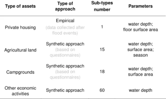
considered—Merz et al. (2010) present the other types of damages that should be estimated for a more complete analysis. Damage functions were used (Table 3), which depend mainly on the following parameters: type and floor surface area of the exposed object, average water depth, and season of occurrence (campgrounds and agriculture). Flood velocity and flood duration were considered to be homogeneous. These damage functions were taken from the recommendations of the French State (MEDDTL, 2011). For a complete description, see the original study (Grelot et al., 2012). In the end, a total of 94 depth-damage relationships were used, one for each land use type and subtype.
Average Annual Avoided Damages
The average annual damage cost from flooding (AAD [€/year]) is a common performance indicator used to measure potential flood damages over a given territory (Arnell, 1989; Messner et al., 2006). It is equal to the area under the damage-frequency curve, which is the graph of damage D against exceedance frequency f = 1/T:
∫
01D
(
f
)
df
=
AAD
(1)To assess the benefits of the flood risk management project launched on the Orb River in 2001, we computed the potential reduction of the average annual damage costs brought by the mitigation measures, i.e., the variation ∆AAD = AAD –
AAD’from the present to the future situation. This Average Annual Avoided Damage (∆AAD [€/year]) is also equal to:
∫
∆
∆
10
D
(
f
)
df
=
AAD
(2)It can be computed from the range of flood scenarios e1 to e6 and corresponding avoided damages ∆D1 to ∆D6 by
estimating the integral (Eqn 2) with a simple trapezoidal rule (Figure 3).
Net Present Value of the mitigation measures
The last step of the NOE modelling chain is the cost-benefit analysis, which evaluates the efficiency of the flood mitigation measures by comparing their costs with their expected benefits. The costs of the mitigation measures include the initial investment (CI= 35.2 M€) and maintenance costs (CM= 1.6 M€/year). The benefits of the project are measured by the ∆AAD indicator. The Net Present Value (NPV [€]) of the flood mitigation measures is then calculated by comparing the discounted costs and benefits over a time period of R = 30 years (Eqn 2).
(
)
∑
= × − ∆ + − = R i i CM AAD CI NPV 0 τ (3)where τi is the discount coefficient for year i. A positive NPV value means that the benefits generated by the flood risk
Figure 3
Uncertainty and sensitivity analysis
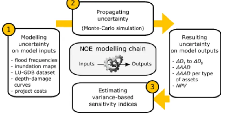
Uncertainty and sensitivity analyses of the NOE modelling chain (Figure 4) were performed using variance-based global sensitivity analysis approach (Saltelli et al., 2008). In the first step of the analysis, sources of uncertainty in the NOE modelling chain were identified and modelled in a probabilistic framework, and a set of random realisations was sampled for each uncertain modelled input. Next, pseudo-Monte Carlo simulations were used to explore the space of input uncertainty and assess the resulting variance of model outputs (∆AAD and NPV indicators). Finally, variance-based sensitivity indices were computed to rank the sources of uncertainty, depending on their contribution to the variance of output indicators.
Modelling sources of uncertainty
Table 4 lists the epistemic uncertainty sources that we took into account in the uncertainty and sensitivity analyses of the NOE modelling chain. Each source of uncertainty was modelled in a probabilistic framework using measurement or expert opinion.
Flood frequency analysis
Uncertainty in the flood frequency analysis may arise from i) stream gauge measurement errors (Neppel et al., 2009); ii) possible non-stationarity of the series due to climate change (Khaliq et al., 2006) and iii) uncertain fitting of a discharge-frequency (Q-f) relationship to the AMFS 1967-2009 dataset (Countryman and Tustison, 2008). Here, only the latter uncertainty was modelled and simulated. After a log transformation leading to the usual linear regression context, standard joint distributions (Maidment, 1993) for the parameters of the fitted Gumbel curve were calculated (Figure 5). A set of n1 = 103 Gumbel curves was then randomly sampled from the parameter joint distribution. From this set of curves, 103 exceedance frequencies fi and according return intervals Ti = 1/fi (Figure 6) were generated for each discharge value qi (i =
1 to 6).
Flood hazard modelling
Another major source of uncertainty in the NOE modelling chain is the inundation mapping process, which includes hydraulic modelling and combination with a high-resolution DTM, to derive water depth maps H(e2) to H(e6) and H(e2’)
to H(e6’). For the sake of simplicity, a restrictive choice was assumed in considering the error on the high-resolution
Digital Terrain Model as the single uncertainty source in water depth maps. Including more detailed descriptions of the hydraulic uncertainties in this study was impossible as the ISIS hydraulic model used for initial flow simulations was not available to us. This choice may be partly justified by the findings of both Bales and Wagner (2009) and Koivumäki et al. (2010), who investigated the various sources of error encountered in this process and conclude that high-resolution topographic data is the most important factor required for accurate inundation maps. The DTM—a raster surface of 5 m cell size—was initially built by stereo-photogrammetry. Both measurement errors and interpolation errors affect the quality of this input data (Wechsler, 2007). These errors were modelled by a Gaussian noise without spatial correlation, whose characteristics were determined from a set of 500 control field points (mean = 0 cm, s.d. = 17 cm). A set of n2 = 100
random realisations of the Gaussian random error field was generated and added as « noise » to the initial water depth maps H(e2) to H(e6) and H(e2’) to H(e6’). We may note that this procedure induces independent variations of the water
levels for each exposed asset; it differs from the study of de Moel and Aerts (2011), who described uncertainty in the water levels with a spatially uniform bias.
Flood exposure modelling
The third source of uncertainty is the location and attribute data errors in the LU-GDB dataset (Koivumäki et al., 2010). The error in the land use GIS layer may stem from the following: i) misclassification of polygonal features representing assets; ii) error on the ground floor elevation of buildings; and iii) error on the surface area of features. Other sources of uncertainty were identified:geometric errors (Bonin, 2006; Girres, 2010), errors in the asset locations, and the evolution of land use over time (Te Linde et al., 2011). Although in some studies (de Moel and Aerts, 2011) the uncertainty of the land use data was represented by using a small number of different datasets, here each uncertainty source was modelled in a probabilistic setting. To describe the misclassification of polygonal features, which may arise in the process of photo-interpretation, a confusion matrix (Fisher, 1991) was built based on expert opinion, giving a confusion probability pa,b for each pair of land use types (a,b) (Table 5). Then, to model the variability of the ground floor elevation
of buildings, measurements were taken during a field survey on a sample of 100 buildings. The study area was divided into five homogeneous zones; in each zone, the distribution of ground floor elevation was described by an empirical
histogram (Figure 7). Random ground floor elevation was also attributed to campgrounds, plots of agricultural land and other economic activities (Table 4). Next, the surface area of the buildings was also randomised, as the features area extracted from cadastral maps differ from the effective surface area of buildings that should be taken into account for flood damage estimation (e.g., wall width should be subtracted). To cope with this issue, the nominal surface of each building was multiplied by a corrective random coefficient drawn independently in a uniform pdf in [0.75; 0.85], considering a digitalising error of 0.3 mm at the map scale (Hengl, 2006). Finally, from this probabilistic description of the uncertainty in the LU-GDB dataset (confusion matrix, empirical distribution of ground floor elevations, corrective coefficient for surface areas), a set of n3 = 1 000 random LU-GDB datasets was sampled.
Figure 6
Damage estimation
The fourth uncertain model input is the set of 94 depth-damage curves (one for each land use type and subtype) used for the damage estimation. Uncertainty about the damage functions has been extensively discussed in previous studies (Koivumäki et al., 2010; Kutschera, 2009; Merz et al., 2004, 2010; Merz and Thieken, 2009; de Moel and Aerts, 2011). In these papers, uncertainty was mainly represented by using two or three different sets of damage functions coming from various studies. Only de Moel and Aerts (2011) used a parametric uncertainty model (beta pdf) derived from Egorova et al. (2008). Here, to treat all uncertainty sources in a probabilistic framework, we made the choice to use a single set of depth-damage curves and represent their uncertainty by a uniform pdf, defining a -50% to +50% uncertainty range around nominal curves (Figure 8). Depth-damage curves associated with each land use type and subtype were assumed to vary independently—contrary to de Moel and Aerts (2011), where they were sampled collectively from a single p-value. A total of n4 = 1 000 random sets of depth-damage relations was sampled this way.
Figure 7
Project costs
Finally, the last source of uncertainty in the NOE modelling chain is related to the costs of the flood risk management project. Based on expert opinion, investment costs CI and maintenance costs CM were assumed to follow a triangular pdf with the parameters shown in Table 4.
Propagating uncertainty
Once uncertainty had been modelled for each source of uncertainty, it was propagated through the NOE modelling chain using Monte Carlo simulation and a specific sampling scheme following Lilburne and Tarantola (2009). It uses two independent quasi-random LP-τ matrices A and B (Sobol, 1967), here of length Nbase=4 096—this sampling size was
chosen to fill the necessary conditions for the LP-τ samples (Nbase must be a power of 2) and large enough to obtain a
satisfactory level of accuracy for the sensitivity indices estimates. These two matrices were combined through several permutations to explore the uncertainty domain of the five model inputs considered, respectively: exceedance frequencies; inundation maps; LU-GDB dataset; depth-damage curves; and project costs. The ith line of sample A or B is a set (l1(i)
, l2(i), l3(i), l4(i) ,l5(i)) where each li(i) is a random integer label sampled from {1, ..., nj} associated with a single random realisation of the jth model input (from the set of nj random realisations that was previously generated). One can note that the number
nj of random realisations is not the same for each model input: these numbers were chosen under the constraints of CPU time and storage space. Next, the NOE modelling chain was run for each line of samples A, B and a number of combinations of A and B—more details on the procedure can be found in Lilburne and Tarantola (2009). The total number of model runs was Ntot = 28 672 (this number depends on the initial sample size Nbase and the number of uncertain model
inputs considered) for a total CPU time of 24 hours on a 6-nodes cluster computer.
Variance-based sensitivity indices
Uncertainty propagation results in a set of Ntot = 28 672 values for the following outputs of interest:
- avoided flood damages per scenario (∆D1 to ∆D6)
- Average Annual Avoided Damages (∆AAD)
- Average Annual Avoided Damages per type of assets - Net Present Value of mitigation measures (NPV)
Then, the variance-based total-order sensitivity indices of each source of uncertainty with respect to each output of interest were estimated using the expressions given by Lilburne and Tarantola (2009). These sensitivity indices, denoted by STi,
measure the contribution of a given source of uncertainty, denoted by Ui, and all its interactions with other sources of
uncertainty, denoted by U~i, to the variance of a given model output, denoted by Y:
[
]
(
)
( )
Y
Var
U
Y
Var
E
=
ST
i ~i (3)STi is the expected part of output variance Var(Y) that would remain if all sources of uncertainty but Xi were fixed. Please
refer to Saltelli et al. (2008) for more details on global sensitivity analysis and the estimation of sensitivity indices.
Results
Uncertainty analysis
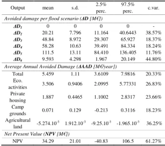
Table 6 summarises the outcome of the uncertainty analysis. For each output of interest, it gives descriptive statistics over the Ntot = 28 672 model runs. It displays mean values of avoided damages per flood scenario, ranging from 9.593 M€ to
111.5 M€. The largest avoided damage is reached for scenario e5(100-year design flood), with a total reduction ∆D5 =
111.5 M€, whereas the mitigation measures performed worst for the extreme flood scenario e6, with a mean avoided
damage ∆D6 = 9.593 M€ and a negative minimum value of -4.695 M€, meaning that the damage costs might increase from
the present to the future situation for this scenario. The Average Annual Avoided Damage indicator shows a mean value of
∆AAD = 5.459 M€/year. Table 6 clearly suggests that the contribution of the four types of assets to this total indicator is
uneven: while the economic activities and private housing account respectively for 64% and 34% of the total ∆AAD, the share of campgrounds and cultivated land is only equal to 1.3% and 0.7%, respectively. Finally the effect of the flood mitigation measures appears to be heavily dependent on the type of assets considered. Despite all input uncertainties, the
∆AAD indicator on private housing and economic activities (other than agriculture and campgrounds) prove to be always
positive in this uncertainty analysis. In contrast, the mitigation measures will most likely result in an increase in the average annual damage for agricultural land as ∆AAD is negative in this sector for all model runs. Regarding campgrounds, no conclusion can be drawn from the study as ∆AAD is positive in this sector for only 72.6% of the model runs. It can also be noted that all flood damage indicators display a coefficient of variation ranging from 11.76% to 44.80%.
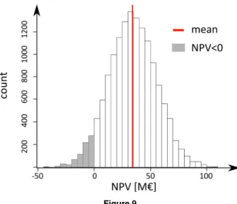
Finally, Figure 9 shows the empirical distribution of the Net Present Value of the flood mitigation measures over Ntot =
28 672 simulations. With a mean value of +34.29 M€, the flood risk management project seems to be a sound investment. The NPV indicator also appears to be positive for 96% of model runs, which we interpret to mean that despite all the uncertainty sources that were considered in the NOE modelling chain, the benefits of the flood mitigation measures still prove to almost certainly outweigh their costs.
Sensitivity analysis
The total order variance-based sensitivity indices were computed for each uncertain model input with respect to each output of interest (Table 7). First, the variance of the total ∆AAD indicator can be observed to be almost equally explained by the uncertainty in the exceedance frequencies, water depth maps, depth-damage curves and LU-GDB dataset, with sensitivity indices ranging from 0.18 to 0.33. No main source of uncertainty can be identified, meaning that they are in a sense “well-balanced”.
However, sensitivity indices with respect to the partial ∆AAD indicator for each economic sector give a very different picture. The variance of ∆AAD on private housing appears to be mainly explained by the uncertainty of the depth-damage curves (sensitivity index: 0.78). For campgrounds and agricultural land, the depth-damage curves also prove to be the most important source of uncertainty (sensitivity index: 0.6 and 0.4, respectively), followed by the uncertainty of the LU-GDB dataset (sensitivity index: 0.38 for both sectors).
Figure 10
In addition, for private housing, agricultural land and campgrounds, the uncertainty in the water depth maps is almost non-influential (sensitivity index < 0.02), while it is the second most important source of uncertainty for other economic activities (sensitivity index: 0.38). Finally, Table 7 also indicates that the variance of the Net Present Value of flood mitigation project is mainly due to the uncertainty on its benefits (measured by total ∆AAD) rather than the uncertainty on its costs, which contribute to only 12% of the NPV variance.
To further identify the factors that explain the variance of ∆AAD indicator, sensitivity analysis can also be based on a graphical analysis. Figure 10 displays the sampled flood exceedance frequencies f1 to f6 against the estimated avoided
damages ∆D1 to ∆D6 for all Ntot = 28 672 model runs, along with the curves associated with the nominal, minimum and
maximum values of the ∆AAD indicator, which is equal to the area under the curve. It may be noted that as the damage and frequency estimates of each flood scenario are correlated, the extremum values of the ∆AAD indicator do not always correspond to the extremum points in the damage-frequency graph for all flood scenarios. Figure 9 supports the conclusion that the variance of the ∆AAD indicator is mainly due to the uncertain position of scenarios e1 (first flood event where the
damage to property begins) and e2 (10-year design flood) on this damage-frequency graph. Flood scenarios e3 to e5 show a
larger dispersion of estimated avoided damages, but their position on the x-axis (exceedance frequency) is less spread; hence their contribution to the total variance of the ∆AAD indicator is small.
Discussion
Assessing robustness of a flood risk CBA study
Our first goal was to assess the robustness of the cost-benefit analysis of the structural flood mitigation measures on the Orb River through an uncertainty analysis of the NOE modelling chain. Our approach was strongly motivated by prior publications in which uncertainty analysis was used to evaluate the robustness of flood damage assessments. We completed these works by propagating uncertainty up to the cost-benefit analysis of the flood mitigation measures, which had not been performed before. We obtained empirical descriptive statistics for the two CBA-AD outcomes, the Average Annual Avoided Damages and the Net Present Value of flood mitigation measures, displaying quite large coefficients of variation of 20.33% and 61.27%, respectively. The visualisation of the Monte Carlo simulations on a damage-frequency graph (Figure 10) gave us a new insight on the robustness of the ∆AAD indicator, proving that its variance is mainly explained by the uncertain characterisation (in terms of exceedance frequency and estimated damages) of flood scenarios with small return intervals (5 and 10-year floods). We also found (Figure 9) that the probability of the project costs outweighing the project benefits appears to be lower than 5%. We are convinced that these results may prove useful to provide water managers and stakeholders with a more complete picture on the cost-benefit analysis and the associated uncertainty, even though we know that they are usually untrained in coping with the uncertainty related to scientific information in flood risk studies (Morss et al. 2005).
Improving the NOE modelling chain
Our research also sought to identify the main sources of uncertainty in the NOE modelling chain to find ways to improve it. Although variance-based sensitivity analysis is widely used for that purpose in many disciplines, it had never been applied, to our knowledge, to a CBA-AD of flood control measures. We demonstrated the use of Sobol' sensitivity indices (Table 7) to rank the sources of uncertainty, depending on their contribution to the variance of the ∆AAD and NPV indicators. A first conclusion is that, on a global scale, sources of uncertainty are well-balanced, meaning that they all explain a significant share of the variance of the ∆AAD and NPV indicators. Yet, more useful lessons can be learnt from looking at each economic sector separately. The uncertainty on the depth-damage curves proved to be the key factor that
explains the variance of the average annual damages on private housing, campgrounds and agricultural land. This result is in line with those of Apel et al. (2008) and de Moel and Aerts (2011), who found that in damage assessment of a single flood event, the choice of damage functions is a much more important factor than the choice of a hazard model. It thus supports the conclusion that improving the depth-damage curves and more generally the damage functions are priorities to make more robust flood damage assessments in these sectors. Our results also indicate that there is almost a third of the variance of the ∆AAD and NPV indicators that cannot be reduced as it stems from the variance of the flood return interval estimates. This observation corroborates the conclusions of Apel et al. (2004), who stated that reliable extreme value statistics were crucially important for reducing the uncertainty of the risk assessment. Unfortunately, reducing this input uncertainty would require longer time series of maximum discharges at Tabarka gauging station, which are not available. Finally, the uncertainty on the floor elevation of buildings proved to have a negligible contribution to the variability of the annual damage estimates for private housing. This finding fits well with the results of Koivumäki et al. (2010), who showed that adding a single elevation value per building was inadequate to obtain more accurate damage estimates. Of course, these findings are specific to the Orb River study site: in a different case-study, ranking of the various uncertainty sources may be significantly different.
Averaging-out effects
The sensitivity analysis also provided an interesting insight on how the uncertainty on inundation maps influence the variance of damage estimation. Our results offer evidence that improving water depth estimation would be of almost no use in reducing variance of ∆AAD estimates for campgrounds, agricultural land and private housing, while it is the second most important source of uncertainty for other economic activities. This finding is in apparent conflict with the conclusions of Apel et al. (2004, 2008) or de Moel and Aerts (2011), who reported that uncertainty in the water depths is less important than other uncertainty sources without distinction of the economic sector considered. This discrepancy may be explained by two different “averaging-out effects”: one based on the surface area of assets and the other based on the number of assets. On one hand, campgrounds and agricultural land have a large surface area compared with other types of assets (33 000 and 9 000 sq. m. in average, Table 2): as a result, the error on water depths, if unbiased, is reduced when it is averaged over the large surface area of these assets. Hence, for both sectors, the contribution of the water depth maps to the variance of the ∆AAD indicator is low. On the other hand, the polygonal features classified as “private housing” or “economic activities” have a rather small surface area (83 sq. m. and 904 sq. m. on average, respectively), and the uncertainty in the average water depth for each individual asset is thus large. Nevertheless, the number of features classified as “private housing” (16 436) is much larger than the number of assets classified as “other economic activities” (691), which results in a “number averaging-out effect”: the dispersion of water depth errors is averaged over the large number of housing polygons scattered across the study area. A similar “number averaging-out effect” may partly explain why the uncertainty on depth-damage curves appears to be more influential on the private housing sector, which is described with only one depth-damage curve, than for the other economic activities, which are described by 60 damage curves that are assumed to vary independently. These findings support the conclusion that various averaging-out effects (related not only to the surface area of assets and the number of assets but also to the number of land use types considered, the number of damage functions used, etc.) control the ranking of the uncertainty sources in the NOE modelling chain.
Saint-Geours et al. (2012) discussed this issue from a theoretical point of view and showed that the ranking of the uncertainty sources is closely related to the spatial support (and thus to the scale) of the model output. This result is in agreement with the call of Koivumäki et al. (2010) for further research on what constitutes a reasonable ‘scale-accuracy relationship’ in flood damage assessments: our results suggest that the ‘scale-accuracy-sensitivity’ relationship must be further investigated.
Limits
It should be noted that our work is based on hypotheses that may limit the strength of some of its results. First, some sources of uncertainty were identified in the NOE modelling chain but not taken into account in the uncertainty and sensitivity analysis: the evolution of land use over the next thirty years, errors arising from uncertainty on friction coefficients in hydraulic modelling, errors on the location and shape of polygonal features in the LU-GDB dataset, etc. Why were they ignored? Because the data required to rigorously characterise them in a probabilistic framework were not available. Even if we can assume that some of these uncertainty sources would prove to be negligible in the NOE modelling chain, (e.g., errors on the location of assets in the LU-GDB dataset), others are definitely not (e.g., biased errors in hydraulic modelling).
Moreover, even for those sources of uncertainty that were included in the study, the models of uncertainty are sometimes only based on expert opinion. The results of our study heavily depend on such uncertainty parameters. To cope with this issue, a second-level uncertainty analysis could be performed by exploring how the output uncertainty and the sensitivity indices change for given sets of uncertainty parameters.
Conclusion
This work was performed with a view toward promoting the use of Monte Carlo uncertainty analysis and variance-based sensitivity analysis in flood damage assessments and related CBA-AD through a case-study on the Orb Delta, France. For this case-study, we derive the following main conclusions:
(1) Monte Carlo uncertainty analysis allows empirical pdf and confidence bounds on the economic indicators of a cost-benefit analysis applied to flood mitigation measures to be computed.
(2) The variance of the Average Annual Avoided Damages is mainly due to the uncertain characterisation of flood scenarios with small return intervals.
(3) Approximately one-third of the variance of the ∆AAD and NPV indicators cannot be reduced as it stems from a flood frequency analysis based on short time series.
(4) The ranking of uncertainty sources depend on the economic sector considered (private housing, agricultural land, economic activities)
(5) Uncertainty in the depth-damage curves is a prominent factor for computing the ∆AAD for private housing and agricultural land.
(6) The ranking of uncertainty sources is influenced by various averaging-out effects that depend on the number and surface area of the assets considered, the number of land use types, the number of damage functions, etc.
Further research is now needed to extend the reach of our study by trying to reduce the uncertainty in the input data identified as being influential in the study and including in the analysis uncertainty sources that were ignored so far.
Acknowledgements
The flood-related data have been kindly provided by the Syndicat Mixte de la Vallée de l'Orb (Laurent Rippert) and the Syndicat Béziers-la-Mer (Pierre Enjalbert).
References
Apel H., Thieken A.H., Merz B. & Blöschl G. Flood risk assessment and associated uncertainty. Nat Hazards Earth Syst Sci 2004, 4, 295–308.
Apel H., Merz B. & Thieken A.H. Quantification of uncertainties in flood risk assessments. Int J River Basin Manage 2008, 6, (2), 149–162.
Apel H., Aronica G.T., Kreibich H. Flood risk analyses-how detailed do we need to be? Nat Hazards 2009, 49 (1), 79–98. Arnell N.W. Expected annual damages and uncertainties in flood frequency estimation. J Water Resour Plann Manage 1989,
115, 94–107.
Ascough J.C., Maier H.R., Ravalico J.K. and Strudley M.W. Future research challenges for incorporation of uncertainty in environmental and ecological decision-making. Ecol Model 2008, 219, 383–399.
Bales J. & Wagner C. Sources of uncertainty in flood inundation maps. J Flood Risk Manage 2009, 2, 139–147
BCEOM & Syndicat Mixte de la Vallée de l'Orb. Etude de gestion du risque inondation dans le bassin versant de l’Orb. 2000. Bianchi M. & Zheng C. SGeMS: a free and versatile tool for three-dimensional geostatistical applications. Ground water 2009,
47, 8–12.
Bernardara P., de Rocquigny E., Goutal N., Arnaud A. & Passoni G. Uncertainty analysis in flood hazard assessment: hydrological and hydraulic calibration. Can J Civ Eng 2010, 37, 968–979.
Bonin O. Sensitivity analysis and uncertainty analysis for vector geographical applications 7th International Symposium on
Spatial Accuracy Assessment in Natural Resources and Environmental Sciences 2006.
Cariboni J., Gatelli D., Liska R. & Saltelli A. The role of sensitivity analysis in ecological modelling. Ecol Model, 2007, 203, 167–182
Castrignano A. Accuracy assessment of digital elevation model using stochastic simulation. In: M. Caetano & M. Painho, eds.
Proc 7th International Symposium on Spatial Accuracy Assessment in Natural Resources and Environmental Sciences 2006.
Council of European Communities. Directive 2007/60/EC of the European Parliament and of the Council of 23 October 2007 on the assessment and management of flood risks. Official J 2007, 27–34.
Countryman J.D. & Tustison B. Flood frequency confidence bounds - Art, science or guess. In: Proceedings of the World
Environmental and Water Resources Congress 2008 2008, 316.
European Commission. Impact assessment guidelines. 2009, #SEC(2009) 92
European Commission. Guide to cost-benefit analysis of Investment Projects. Evaluation Unit, DG Regional Policy 2008. EEA, WHO, JRC. Impacts of Europe’s changing climate—2008 indicator-based assessment. EEA No 4/2008. European
Boardman N.E. Cost-benefit analysis, concepts and practice. (3 ed.). Upper Saddle River, NJ: Prentice Hall, 2006.
Deutsch C.V. & Journel, A.G. GSLIB: geostatistical software library and user’s guide. New York: Oxford University Press, 1998.
Egorova R., Van Noortwijk J.M. & Holterman S.R. Uncertainty in flood damage estimation. Int J River Basin Manage 2008, 6, 139–148.
Erdlenbruch K., Gilbert E., Grelot F. & Lescouliers, C. Une analyse coût-bénéfice spatialisée de la protection contre des inondations: application de la méthode des dommages évités à la basse vallée de l'Orb. Ingénieries
Eau-Agriculture-Territoires 2008, 53, 3–20.
Fisher P.F. Modelling soil map-unit inclusions by Monte Carlo simulation. Int J Geo Inf Science 1991, 5, 193–208
Girres, J. & Julien, P. Estimation of digitizing and polygonal approximation errors in the computation of length in vector databases. In: Tate NJ, Fisher PF (eds) Proceedings of Accuracy2010—The ninth international symposium on spatial
accuracy assessment in natural resources and environmental sciences, 85–88.
Gouldby B.P., Sayers P.B., Panzeri M.C. & Lanyon J.E. Development and application of efficient methods for the forward propagation of epistemic uncertainty and sensitivity analysis within complex broad-scale flood risk system models. Can J Civ
Eng 2010, 37, 955–967.
Grelot F., Enjalbert P., Agenais A.-L., Bailly J.-S., Brémond, P., Langer, T. and Saint-Geours, N. Programme d'actions de prévention des inondations sur les bassins versants de l'Orb et du Libron. Compléments à l'étude ACB de 2007. 2012. Helton J. & Davis F. Latin hypercube sampling and the propagation of uncertainty in analyses of complex systems. Reliab Eng
Syst Safe 2003, 81, 23–69.
Hengl T. Finding the right pixel size. Comp Geosci 2006, 32, 1283–1298 ISIS user guide. Available at www.halcrow.com.isis. (accessed 12 May 2012).
INSEE. French classification of activities – NAF Rev. 2 2008. Available at www.insee.fr/en/methods/default.asp?page =n omenclatures/naf2008/naf2008.htm (accessed 12 May 2012).
Khaliq M.N., Ouarda T.B.M.J., Ondo J.-C., Gachon P. & Bobée B. Frequency analysis of a sequence of dependent and/or non-stationary hydro-meteorological observations: a review. J Hydrol 2006, 329, (3-4), 534–552.
Koivumäki L., Alho, P., Lotsari, E., Käyhkö, J., Saari, A. & Hyyppä, H. Uncertainties in flood risk mapping: a case study on estimating building damages for a river flood in Finland. J Flood Risk Manage 2010, 3, 166–183.
de Kort I.A.T. & Booij M.J. Decision making under uncertainty in a decision support system for the Red River Env Model Soft 2007, 22, 128–136.
Kutschera, G. What are the uncertainties when calculating flood damage potentials? Wasser Wirtschaft 2009, 99, 21–27. Lilburne L. & Tarantola S. Sensitivity analysis of spatial models. Int J Geo Inf Sci 2009, 23, (2), 151–168.
Maidment, D.R. Handbook of Hydrology. New York: McGraw-Hill, 1993.
MEDDTL. Programmes d'action de prévention des inondations (PAPI). De la stratégie aux programmes d'action. Cahier des charges. Ministère de l'Écologie, du Développement durable, des Transports et du Logement 2011.
Merz B., Kreibich H., Thieken A. H. & Schmidtke R. Estimation uncertainty of direct monetary flood damage to buildings. Nat
Hazards Earth Syst Sci 2004, 4, 153–163.
Merz B., Kreibich H., Schwarze R. & Thieken A. Assessment of economic flood damage. Nat Hazards Earth Syst Sci 2010, 10, 1697–1724.
Merz B., Thieken A.H. Flood risk curves and uncertainty bounds. Nat Hazards 2009, 51, (3), 437–458.
Messner F., Penning-Roswell E., Green C., Meyer V., Tunstall S. & van der Veen A. Guidelines for socio-economic flood damage evaluation. Report Number T09-06-01, FLOODsite, 2006.
de Moel H. & Aerts J. Effect of uncertainty in land use, damage models and inundation depth on flood damage estimates. Nat
Hazards Earth Syst Sci 2011, 58, 407–425.
de Moel H., Asselman N.E.M. and Aerts, J.C.J.H. Uncertainty and sensitivity analysis of coastal flood damage estimates in the west of the Netherlands. Nat Hazards Earth Syst Sci 2012, 12, 1045–1058.
Morss R.E., Wilhelmi O.V., Downton M.W. & Gruntfest E. Flood risk, uncertainty, and scientific information for decision making. Bull Am Meteorol Soc 2005, Nov, 1593–1601.
Mostert E. & Junier S.J. The European flood risk directive: challenges for research. Hydrol Earth Syst Sci Discussions 2009, 6, 4961–4988.
Neppel L., Renard B., Lang M., Ayral P., Coeur D., Gaume E., Jacob N., Payrastre O., Pobanz K. & Vinet F. Flood frequency analysis using historical data: accounting for random and systematic errors. Hydrol Sci J 2010, 55, 192–208.
Pappenberger F. & Beven K.J. Ignorance is bliss: Or seven reasons not to use uncertainty analysis. Water Resour Res 2006, 42, W05302.
Pappenberger F., Harvey H., Beven K., Hall J. & Meadowcroft I. Decision tree for choosing an uncertainty analysis methodology: a wiki experiment. Hydrol Process 2006, 20, 3793–3798.
Pappenberger F., Beven K.J., Ratto M. & Matgen P. Multi-method global sensitivity analysis of flood inundation models. Adv
Water Resour 2008, 31, 1–14.
Plan Rhône – Volet Inondations. Analyse Coût-Bénéfice: un outil d’aide à la décision pour optimiser les projets de prévention
des risques d’inondation. 2010. Available at www.planrhone.fr/extern/00002/ACB/docs/DREAL_ACB_guide.pdf. (accessed
12 May 2012).
Refsgaard J.C., van der Sluijs J.P., Højberg A.L. & Vanrolleghem P.A. Uncertainty in the environmental modelling process: a framework and guidance. Environ Modell Softw 2007, 22, 1543–1556.
de Rocquigny E. An applied framework for uncertainty treatment and key challenges in hydrological and hydraulic modeling.
Can J Civ Eng 2010 37, 941–954.
Saint-Geours N., Lavergne C., Bailly J.-S., Grelot, F. Change of support in variance-based sensitivity analysis. Math Geosci 2012, Online first.
Saltelli A., Ratto M., Andres T., Campolongo F., Cariboni J., Gatelli D., Saisana M. & Tarantola S. (eds). Global sensitivity analysis, the primer. New York:Wiley, 2008.
Saltelli A., Annoni P., Azzini I., Campolongo F., Ratto M. & Tarantola S. Variance based sensitivity analysis of model output: design and estimator for the total sensitivity index. Comput Phys Commun 2010, 181, 259–270.
SMVOL. Programme d'actions de prévention des inondations sur les bassins de l'Orb et du Libron pour les années 2011 à 2015. Note de présentation. Syndicat Mixte des Vallées de l'Orb et du Libron. 2011.
Sobol I.M. Distribution of points in a cube and approximate evaluation of integrals. U.S.S.R Comput Maths Math Phys 1967, 7, 86–112.
Stephens E., Bates P., Freer J. & Mason D. The impact of uncertainty in satellite data on the assessment of flood inundation models. J Hydrol 2012, 414-415, 162 – 173.
Tarantola S., Giglioli N., Jesinghaus J. & Saltelli A. Can global sensitivity analysis steer the implementation of models for environmental assessments and decision-making? Stoch Env Res Risk Ass 2002, 16, 63–76.
Te Linde A., Bubeck P., Dekkers J.E.C., de Moel H. & Aerts J. Future flood risk estimates along the river Rhine Nat Hazards
Earth Syst Sci 2011, 11, 459–473.
Torterotot, J.-P. Le coût des dommages dus aux inondations: Estimation et analyse des incertitudes. PhD Thesis, École Nationale des Ponts et Chaussées, Paris, France, 1993.
US Environmental Protection Agency (2009) Guidance on the development, evaluation, and application of environmental models. Council for Regulatory Environmental Modeling. Available at http://www.epa.gov/crem/library/ cred_guidance_0309.pdf. (accessed 17 April 2012).
Walker W., Harremoees P., Rotmans J., van der Sluijs J.P., van Asselt M., Janssen P. & Krayer von Krauss M. Defining uncertainty: a conceptual basis for uncertainty management in model-based decision support. Integrat Ass 2003, 4, 5–17. Wechsler, S. Uncertainties associated with digital elevation models for hydrologic applications: a review. Hydrol Earth Syst Sci
2007, 11, 1481–1500.
Weichel T., Pappenberger F. & Schulz K. Sensitivity and uncertainty in flood inundation modelling - concept of an analysis framework. Advances in Geosciences 2007, 11, 31–36.
Captions of figures
Figure 1 The study site is located in Hérault département, south of France. The Orb River flows southward.
Source: www.geoportail.fr
Figure 2 Flowchart of the NOE modelling chain
Figure 3 Computation of Average Annual Avoided Damage Figure 4 Flowchart for uncertainty and sensitivity analysis
Figure 5 Annual maximum flow series AMFS 1967-2009 and fitted Gumbel distribution (red solid line) with 95% confidence bounds
(dotted blue lines)
Figure 6 Empirical distributions of return intervals T for flood scenarios e1 to e6
Figure 7 Empirical distribution of the elevation of ground floor of buildings over zones A (top) to F (bottom)
Figure 8 Nominal depth-damage curve for private housing (red solid line) with a [-50%; +50%] uncertainty range (blue dotted lines) Figure 9 Empirical distribution of NPV indicator over Ntot=28672 simulations and mean value (solid line)
Figure 10 Avoided damages against exceedance frequency: nominal curve (solid line), first 500 simulations (dots), curves
Tables
Table 1 Flood scenarios.
Scenario description Max. discharge q [m3/s] Exceedance frequency f [ ] Return interval T = 1/f [years]
e1 that induces damage Smallest flood event 1018 0.2 5
e2 10-year design flood 1287 0.1 10
e3 (December, 1987) Historical flood 1696 0.0333 30
e4 (January, 1996) Historical flood 1882 0.02 50
e5 Large design flood 2133 0.01 100
e6 Probable maximum flood
(over-topping dykes) 3000 0.001 1000
Table 2 Content of land use dataset LU-GDB
Type of assets Data source
Number of objects Total surface [sq. km] Average surface [sq. m]
Private housing Cadastral map
+ field survey 16436 1.37 83 Agricultural land National agricultural land use
statistics (2009) 707 23.36 33044 Campgrounds Cadastral map
+ field survey 111 1.02 9203 Other economic
activities
Cadastral map
+ CCI dataset (2009) 691 0.62 904
Table 3 Damage functions
Type of assets Type of approach
Sub-types
number Parameters
Private housing
Empirical
(data collected after flood events)
1 water depth; floor surface area
Agricultural land Synthetic approach (based on questionnaires) 15 water depth; surface area; season Campgrounds Synthetic approach (based on questionnaires) 18 water depth; surface area Other economic
Table 4 Sources of uncertainty in NOE modelling chain
Model input Nature of uncertainty Modelling uncertainty
(U: uniform pdf)
Sample size n
Hazard maps
H(e1 ) to H(e6 )
Errors in hydraulic modelling Errors in DTM
Only DTM error is considered: Gaussian noise without spatial
correlation (mean = 0 cm, s.d. 17 cm). 100
LU-GDB dataset
● Misclassification of land use types and subtypes ● Variability of ground floor elevation of buildings (lack of data)
● Shape and surface of polygonal features (measurement errors)
● Confusion matrix for land use misclassification.
● Empirical distribution of ground floor elevation of assets from field survey:
- private housing: empirical histograms on five homogeneous zones - campgrounds: U[-0.3m; +0.3m]
- plots of cultivated land: U[-0.2m; +0.2m] - other economic activities: U[0.4m; 0.6m]
● Random multiplying coefficient for surface area of buildings:
U[0.75; 0.85]
1 000
Return intervals
T1 to T6
Lack of data
(short time series of annual maximum discharge). Confidence interval on the fitted Q-f relation 1 000 Depth-damage
curves Lack of data
For each depth-damage curve, random multiplying coefficient εi
drawn from U[0.5; 1.5]. εi are independent. 1 000
Project costs
CI and CM Lack of knowledge
Based on expert opinion.
Triangular distributions with parameters [M€]:
CI (min) = 28.6 ; CI (mode) = 38.6 ; CI (max) =35.2
CM (min) =1.3 ; CM (mode) = 1.6 ; CM (max) =1.8
4 096
Table 5 Confusion matrix of LU-GDB dataset
Land use type Number of
sub-types Probability of confusion between sub-types Private housing 1 No confusion. Agricultural land
15 25% chance of confusion between durum wheat and bread wheat; 10% chance of confusion between colza, maize, barley and sunflower; 25% chance of confusion between permanent and temporary grassland.
Campgrounds 18 No confusion.
Other economic
activities
60 0.17% chance of belonging to each other class of economic activities.
Table 6 Descriptive statistics for each output of interest over Ntot = 28672 simulations
Output mean s.d. 2.5%
perc.
97.5% perc. c.var.
Avoided damage per flood scenario (∆D [M€])
∆D1 0 0 0 0 - ∆D2 20.21 7.796 11.164 40.6443 38.57% ∆D3 48.84 8.972 29.307 65.927 18.37% ∆D4 58.28 10.63 39.491 84.334 18.24% ∆D5 111.5 13.11 84.410 136.405 11.76% ∆D6 9.593 4.298 1.967 20.149 44.80%
Average Annual Avoided Damage (∆AAD [M€/year])
Total 5.459 1.11 3.6109 7.9816 20.33% Eco. activities 3.506 0.9406 2.0995 5.77331 26.83% Private housing 1.887 0.4465 1.1002 2.8317 23.66% Camp grounds 0.071 0.129 -0.213 0.3116 18.23% Agricultural land -5.274.10-3 1.912.10-3 -9.25.10-3 -1.965.10-3 36.25%
Net Present Value (NPV [M€])
NPV 34.29 21.01 -40.83 106.5 61.27%
Table 7 Total order sensitivity indices with respect to the different outputs of interest. Grey cases indicate the most important
sources of uncertainty
Total-order sensitivity index of: Exceed. Prob. Water depths Depth-damage curves LU-GDB dataset Project costs
Average Annual Avoided Damage
Total 0.33 0.29 0.18 0.21 0
Eco. activities 0.4 0.38 0.2 0.3 0
Private housing 0.22 0.005 0.78 0.03 0
Campgrounds 0.2 0.01 0.6 0.38 0
Agricultural land 0.27 0.02 0.4 0.38 0
Net Present Value
W ith r es pe ct to : NPV 0.25 0.18 0.23 0.21 0.12