HAL Id: cea-02509266
https://hal-cea.archives-ouvertes.fr/cea-02509266
Submitted on 16 Mar 2020
HAL is a multi-disciplinary open access
archive for the deposit and dissemination of
sci-entific research documents, whether they are
pub-lished or not. The documents may come from
teaching and research institutions in France or
abroad, or from public or private research centers.
L’archive ouverte pluridisciplinaire HAL, est
destinée au dépôt et à la diffusion de documents
scientifiques de niveau recherche, publiés ou non,
émanant des établissements d’enseignement et de
recherche français ou étrangers, des laboratoires
publics ou privés.
Passive Acoustic Leak Detection for Sodium Cooled Fast
Reactors Using Hidden Markov Models
A. Riber Marklund, S. Kishore, V. Prakash, K. Rajan, F. Michel
To cite this version:
A. Riber Marklund, S. Kishore, V. Prakash, K. Rajan, F. Michel. Passive Acoustic Leak Detection for
Sodium Cooled Fast Reactors Using Hidden Markov Models. ANIMMA 2015 - 4th International
Con-ference on Advancements in Nuclear Instrumentation Measurement Methods and their Applications,
Apr 2015, Lisbon, Portugal. �10.1109/ANIMMA.2015.7465560�. �cea-02509266�
Passive Acoustic Leak Detection for Sodium Cooled
Fast Reactors Using Hidden Markov Models
A. Riber Marklund, S. Kishore, V. Prakash, K. K. Rajan, F. Michel
Abstract – Acoustic leak detection for steam generators of
sodium fast reactors have been an active research topic since the early 1970s and several methods have been tested over the years. Inspired by its success in the field of automatic speech recognition, we here apply hidden Markov models (HMM) in combination with Gaussian mixture models (GMM) to the problem. To achieve this, we propose a new feature calculation scheme, based on the temporal evolution of the power spectral density (PSD) of the signal. Using acoustic signals recorded during steam/water injection experiments done at the Indira Gandhi Centre for Atomic Research (IGCAR), the proposed method is tested. We perform parametric studies on the HMM+GMM model size and demonstrate that the proposed method a) performs well without a priori knowledge of injection noise, b) can incorporate several noise models and c) has an output distribution that simplifies false alarm rate control.
I. INTRODUCTION
ODIUM fast reactors (SFRs) represent a possible option for reaching the standards for future nuclear power concepts proposed by the Generation IV forum [1]. Inherent in the SFR design are however risks related to the interaction between sodium and water in the turbine circuit. Ongoing research and development performed at the CEA therefore aims to develop a sodium-nitrogen energy conversion system for SFRs. In any case, a leak between the secondary and tertiary sides, i.e. inside steam generators or sodium-nitrogen heat exchangers will remain an accident precursor which has to be detected in a fast and reliable way.
Research on acoustic leak detection (ALD) for this purpose has been ongoing for many years. Both active and passive methods may be needed in the final implementation
Manuscript received March 31, 2015. This study was performed within the framework of a collaboration project between KTH and CEA on the instrumentation and safety of sodium cooled reactors. The work was supported by the Swedish Research Council, grant number B0774801.
A. Riber Marklund is with the Royal Institute of Technology (KTH), currently on secondment to the Commisariat a l’Energie Atomique et aux Energies Alternatives (CEA), Cadarache center DEN/DTN/STCP/LIET Bâtiment 202, 13108 St Paul-lez-Durance, France (telephone: +33 (0)4 42 25 57 26 , e-mail: [email protected]).
S. Kishore is with the Fast Reactor Technology Group of IGCAR (e-mail: [email protected]).
V. Prakash is with the Vibrations Diagnostics Division, Fast Reactor Technology Group of IGCAR (telephone: +91 44 27 48 00 86, e-mail: [email protected]).
K.K. Rajan is with the Fast Reactor Technology Group & and Engineering Services Group of IGCAR (telephone: +91 44 27 48 00 83, e-mail: [email protected]).
F. Michel is with the Commisariat a l’Energie Atomique et aux Energies Alternatives (CEA), Cadarache center DEN/DTN/STCP/LIET Bâtiment 202, 13108 St Paul-lez-Durance, France (telephone: +33 (0)4 42 25 47 84, e-mail: [email protected]).
but here we focus on passive ALD. Some basic system requirements were proposed in 1990 by an IAEA specialists’ meeting on steam generators [2] and here we restate the ones that have an impact on the proposed method:
• The sensitivity should be of the order of a few g/s. • The detection time should be on the order of a few
seconds.
• The false alarm rate should be less than one in two years.
A sensitivity of 1 g/s for detection of a water-into-sodium leak was estimated by the IAEA, based on benchmark tests, to correspond to a signal to noise ratio (SNR) of -17 dB in the noisiest steam generators studied at the time [3]. The SNR is defined as
= 10 (1) where Ps / Pbg is the ratio of signal power to be detected to
that of the background noise.
For a detection system which an output frequency of 1 Hz (in line with the second requirement), the specified false alarm rate corresponds to about 1.6×10⁻⁸. By assuming Gaussian detector output and a 2/3 voting logic between independent channels, this would correspond to a false alarm rate of 1.3×10⁻⁴ for each channel.
Most of the works from the literature on passive ALD for SFRs uses methods where a substantial amount of knowledge on the leak noise to be detected is assumed. This knowledge has been used e.g. to create spectra, autoregressive models or wavelet transforms of the studied signals. The classification into background/injection have then been made using e.g. spectral distance measures, statistical measures, neural networks or support vector machines. See for example [3] and [4] for nice overviews of both classic and recent work on the topic.
However, given the complexity of acoustic signals it is unlikely that detailed leak noise knowledge can be easily credited when designing a system for a new plant. Even the normal background noise of a new plant will not be known beforehand and will be depending both on the operating point of the reactor and other loud systems running nearby. This implies that the detection system will need to be able to recognize several different noise types. To the requirements cited above, we therefore propose the addition of two desirable system properties:
• One part of the detector should be independent of reactor operating point.
• The detector should be able to recognize intermittent noises of normal operation that are not leaks.
The motivation of both these properties is to reduce the amount of false alarms due to expected events such as change of reactor power or operation of components nearby, acoustically coupled to the steam generator, such as valves and pumps.
With the aim of investigating new methods capable of fulfilling all the above mentioned requirements, we here introduce a technique which is new to the field but has been both popular and successful within automatic speech recognition, namely the combination of hidden Markov models (HMMs) and Gaussian mixture models (GMMs).
This article is structured as follows: Section II contains a brief description of the basics of HMMs, GMMs and how they can be used. Then we go on to describing discriminating features based on the PSD in section III.A and introducing our new feature calculation scheme in section III.B. Section IV describes the IGCAR SOWART experiment and the obtained acoustic signals. Parametric studies on the proposed method based on these signals are described in section V and results on the detection performance of the method are shown in section VI. Discussion of the results is provided in section VII while conclusions and suggestions for future work are given in section VIII.
II. HIDDEN MARKOV MODELS
Hidden Markov models are statistical signal models based on the Markov property, i.e. that the probability of passing from one state to another is only dependent on the present state and not on the preceding history of states. Here, we follow along the lines of [5], to explain the basic properties of HMMs. Formally, if states at discrete points in time are labeled sn, then a sequence of states is a Markov sequence if
( | , , … , ) = ( | ) (2) The probabilities for passing from one state to another are gathered in a transition matrix A with components ij > 0
corresponding to the probability of passing from state i to state j in one time step. For a total of N possible states, it is by definition required that
∑ = 1 (3) For a full description of the Markov sequence, an initial state vector, π also needs to be specified, representing the probabilities of starting the sequence in each of the N states.
The creation of a signal model from a Markov process is made by associating the state sequence with the signal output in some way. A hidden Markov model assumes that the states are not directly observable, but that each state has its own output probability distribution of so-called features that can be observed. In audio signal modeling, Gaussian mixture
models are commonly used for this purpose. The distribution
of observable features in each state is then given by a linear combination of M Gaussian distributions, i.e.
( ) = ∑ ( ) / ( ) ( ) ( ) (4)
where bm are weight factors, K is the number of feature
vectors in x, Cm is the covariance matrix of the features and
μm are the Gaussian mean values [6]. The parameters of the
complete model λ(A,B,π) can be estimated by using a
training algorithm, such as the Baum-Welch algorithm, on
observed data [5].
Given a model λ and a sequence of observations x, it is possible to calculate exactly the conditional probability
P(x|λ), i.e. the probability that the observed output is generated by the model λ. This probability can, by Bayes rule, be written
( |λ) = ( |λ) ( | , λ) … ( | … , λ) (5) which can be calculated by a recursive algorithm [4]. Since all the factors are <1, this probability will become very small, even for relatively short feature sequences. For practical implementations, it is therefore advised to work with the logarithm of (5) [6].
III. FEATURES FOR ACOUSTIC LEAK DETECTION
A raw acoustic signal without any obvious piecewise structure is not suitable for direct modeling by the HMM+GMM method. To use this approach, the raw signal will instead have to be transformed in a suitable way, creating features that are characteristic of the monitored sounds. In the following sections, we will introduce a new feature calculation method which allows this to be done on industrial noise signals that, a priori, do not present the same obvious piecewise structure as do e.g. speech signals.
A. Basic Features Based on Power Spectral Density
The Power Spectral Density (PSD) of a signal x(t) is a function in frequency space representing the power transmitted within each frequency band of the signal. An estimate of the PSD during a time T is given by
( , ) = // ( ) (6) By performing successive estimates with a sliding time window it is possible to monitor the spectral evolution of the signal. Each time window may also be subdivided into overlapping sub windows in order to decrease the spectral uncertainty by averaging over several estimates of the PSD. This approach is known as the Welch method [7] and will be used here.
Furthermore, to avoid that the detector reacts on pure signal power changes (which can be expected for reactor operating point changes), we propose a normalization such that
∑ ( , ) = 1. (7) It was suggested in [8] that a sum of the PSD at selected frequencies would be a suitable feature for acoustic leak detection. The frequencies would be selected, before starting the detection system, as those presenting the largest contrast between a known leak/injection signal and a known background signal. This type of leak discriminating feature was called PSDSUM, i.e.
( ) = ∑ ( , ) (8) where n is enumerating the successive time windows of length Tn and Imax is a set of local maxima of
where Xinj and Xbg represent the reference
injection and background noises.
In order to detect signal changes by a P without a priori knowledge on the noise to proposed in [9] to monitor the difference
( , ) = ( , ) ( where Xn(fi,Tn) is the PSD estimated in
window Tn of the monitored signal and
reference PSD. Frequency components are those currently presenting the largest d reference background value. The generali becomes
( ) = ∑ ( ) ( where the set of local maximum devi
Jmax(n) may change over time. Note th
sensitive to all deviations from the referenc
B. A New Feature for the HMM+GMM M
By combining measures on know frequencies and the currently most deviatin propose a new feature that is piecewise i suitable for modeling by HMMs. The pro be written
( ) = , + (
where XR is created from PSDs normalized is a set of local maxima order reference PSD and is an set of lo current deviation from the reference PSD power. The number k enumerates the local 1 representing the largest maximum and so value is equal to the K of (4). The number a shift of one frequency band yields a which is much larger than the expected v density, resulting in a piecewise structure typical evolution of the proposed feature signal change is shown in figure 1.
Fig. 1. Typical feature evolution for a signal with ch structure after about 360 samples.
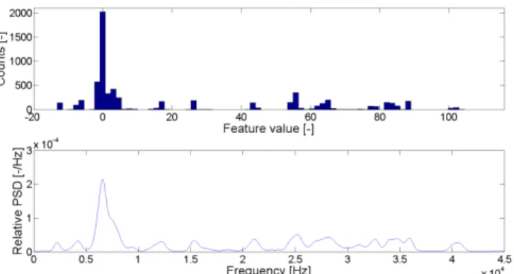
A histogram of the feature will then res shown in figure 2, yielding a link (altho between a noise type and its hidden Markov
e spectra of known PSDSUM approach be detected, it was , ) (10) n the current time
d Xref(fi,Tref) is a e selected online as difference to their ization of (8) then , ) (11) iation frequencies hat this feature is ce.
Method
wn characteristic ng frequencies, we in nature and thus oposed feature can ( )) (12) d according to (7), red by power in a ocal maxima in the D, also ordered by maxima, with k = o on. The largest k is chosen so that total feature shift variation in power e of the feature. A e, demonstrating a
hanging PSD evolution
semble the PSD as ough not obvious)
v model.
Fig. 2. Histogram of a noise model feat the same noise signal (lower panel).
By training a HMM+GMM sequence of a known signal and th model to a test signal by suc logarithm of (5), a detector is obta this detector can be changed by feature sequence used in (5).
The implementation of the featu the HMM+GMM method was mad pattern recognition library develop IV. THE SOWART EXPER
In collaboration between the IG safety of SFR steam generators, a reaction experiments were carried Reaction Test rig (SOWART) fa these experiments, steam/water w through a calibrated injection nozz 9Cr-1Mo steam generator tube. T experiments was to study the effe exposed to the water/steam jet conditions of a SFR system [10].
The acoustic noise generated w accelerometer instrumented wave-section. The obtained recording characterization of the sodium signature and the development of A
In total 10 injections were made conditions given in Table I. T corresponding to all injection cond
TABLE I.INJECTION EXPERIMENT O
Sodium and steam Test ID temperature [°C] SW1 340 SW2 500 SW3 350 SW4 420 SW5 420 SW6 480 SW7 480 SW8 480 SW9 490 SW10 500
ture (upper panel) and the PSD of
on the proposed feature hen reapplying the trained ccessively calculating the ained. The decision time of
varying the length of the ure calculation scheme and de in MATLAB by use of a
ed at KTH [6].
RIMENT (IGCAR)
GCAR and the CEA on the a number of sodium-water d out in the Sodium Water acility of IGCAR [10]. In
was injected into sodium zle, directly impinging on a The main purpose of these ect of wastage on the tube under typical operating was measured using three -guides welded to the test s may be useful in the m-water reaction acoustic
ALD systems.
according to the operating The estimated flow rates ditions were less than 1g/s.
OPERATING CONDITIONS
Steam Injection pressure hole diameter [bar] [mm] 172 0,1 172 0,2 172 0,1 172 0,2 172 0,2 172 0,2 172 0,1 172 0,2 172 0,2 172 0,2
The recordings used in the present study were those of SW1, SW2, SW3, SW4 and SW6. With three channels per test, this yielded in total 15 acoustic signals. As the signals recorded from tests SW9 and SW10 contained too short regions of pure background noise before injection, they were not suitable for the present study. Furthermore, the signals of SW5, SW7 and SW8 were similar to those of SW3 and SW4 and therefore discarded in this study.
V. PARAMETRIC STUDIES
The following signal processing parameters were used: The sampling rate of the SOWART acoustic signals was 200 kHz. Sliding time windows of length T = 10 ms were used and the Welch method was set up with sub windows of 4 ms overlapping each other by 2 ms. Three local maxima were used in (12), i.e. k ranged from 1 to 3.
Each signal was divided into three parts, were the first part served as training data for the background noise model, the middle part (containing the transition between pure background noise and injection noise) served as testing data and the last part served as training data for the injection noise model. The models were trained by the Baum-Welch method to create ergodic, infinite-duration Markov chains with Gaussian mixture output distributions. The training data were segmented by chunks of 100 time windows and the number of (12) was set to 0.3 since this choice was found to provide satisfactory results for a first study.
The remaining free parameters of the presented method were then the number of GMM components and the number of HMM states. The influence of these numbers on the resulting model was studied explicitly by applying trained models on the test signals. In figures 3-4, the resulting log probabilities for SW2 are shown as function of the number of GMM components and HMM states.
Fig. 3. SW2, study of background model log probability as function of the number of GMM components and the number of HMM states
Fig. 4. SW2, study of injection model log probability as function of the number of GMM components and the number of HMM states
The tendency of increased model probability with both the number of GMM components and HMM states was present in all studied signals. However, training problems due to lack of data also appeared, notably with increasing number of GMM components. We therefore chose to work with 3 GMM components and 6 HMM states. For this model size, training problems still occurred occasionally but to an extent that was judged acceptable for this work.
VI. RESULTS
A. Detection Capability in SOWART Data
In figures 6-11, the testing parts of recordings SW1, SW2 and SW6 with corresponding model log probabilities are shown. The detector decision time was set to 1 second. All detector outputs are in the figures normalized to have zero mean and variance one during the first 60 seconds of the signal. In one case, an artificial signal power change before injection was introduced, to demonstrate the detector invariance to such changes.
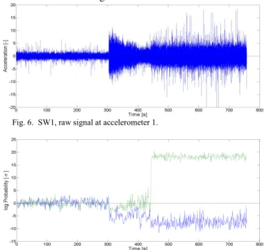
Fig. 6. SW1, raw signal at accelerometer 1.
Fig. 7. SW1, log probabilities of background model (solid line) and injection model (dashed) of the accelerometer 1 signal.
Fig. 8. SW2, raw signal at accelerometer 1. An art introduced before injection.
Fig. 9. SW2, log probabilities of background m injection model (dashed) of the accelerometer 1 signal
Fig. 10. SW6, raw signal at accelerometer 1.
Fig. 11. SW6, log probabilities of background injection model (dashed).
It is clear that both the background an models are fully capable of detecting the being signal power invariant.
Two types of anomalies can be identifi output; the first type is seen for the injecti which seems to initially change in the w SW6, a series of spikes appear before inj
tificial power change is
model (solid line) and l.
model (solid line) and
nd injection noise e injections, while ied in the detector ion model in SW1 wrong direction. In njection, seemingly
correlated with dips in signal ener The first anomaly type will be fu VII while the second type is assum can occur also in a real system.
B. False Alarm Rate
The false alarm rate of a real system based on training of bac dependent both on the statistical output and the long-term characte noise. E.g. if the plant over unrecognized noises, the false alar these noises have been learnt by th magnitude of this problem for a n or less impossible. For the presen study the detector output during t regions and estimate the false ala facility. By concatenating the H detector output before injection in a histogram of this vector, the res analyzed. The resulting raw data v shown in figure 12. Some differen are visible, but it seems reasonabl that the detector output is appro implies that it will be possible to c in a straightforward way. By allo false alarm rate goal of 1.3×10⁻⁴ i
corresponds to a threshold at ab detector output level.
Fig. 12. Raw data and histogram of H output in background region of all testi distribution with equal area is added to the h
C. Detection Capability at Low
We now turn to investigation of as function of SNR. Primarily, w model detector, i.e. the solid line in first measure of detector performan the receiver operating characterist positive rate for a passive ALD sys this area should be close to unity. W as function of the SNR for each tes large region of pure background background + injection noise a positive alarm rates in each region.
rgy seen in the raw signal. urther discussed in section med to be something which
passive acoustic detection ckground noise models is properties of the detector eristics of the background time generates a lot of rm rate will be higher until
he system. To estimate the new reactor system is more nt study, we can however the pure background noise rm rate for the SOWART HMM background model
all test signals and making sulting distribution can be vector and its histogram are nt background noise modes le to make the assumption oximately Gaussian. This control the false alarm rate owing for a 1.5σ drift, the identified in section I then bout 4.5σ from the mean
HMM background model detector ing signals. A standard normal histogram for comparison.
SNR
f the detection performance we study the background n figures 7, 9 and 11. As a nce we take the area under tic (ROC). Since the false stem needs to be very low, We examined this measure st signal by identifying one noise and one region of and simply counting the
As acoustic absorption was seen on several signals, probably due to the appea bubbles in the sodium, the SNR was es PSDs according to:
= 10 (
where Pinj+bgis the signal power in the in
is the signal power in the background regi absorbed acoustic power during injectio power was crudely estimated as the tot decrease in the frequencies where the inje was smaller in magnitude than the backgrou The area under ROC as function background noise deviation detector with one second is shown in figure 13.
Fig. 13. Area under ROC curve as function of SN model detector with 1 s decision time. The maximal a is normalized to be 1. The data points at negative created by adding the background noise vector with the training and testing signals.
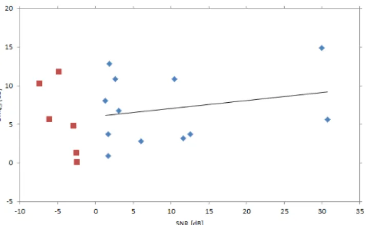
From figure 13 it is clear that the detecto acceptable for all studied recordings, but it deduce any trend towards lower SNRs. detection margin respecting the false al analogy with the one of [3], as:
. = 20
where ds and dbg are the average detector
injection and background regions of detection margin is shown as function of SN
Three outlier points at significantly margin were omitted from the figur represented cases where training pro resulting in a large or even positive log p background noise. Furthermore, six additio negative SNR were created artificially. Thi adding a circular repetition of the backgr with arbitrary phase shift to the training and the six raw data points at lowest SNR.
injection onset in arance of hydrogen stimated from the
)
(13) njection region, Pbg
ion, and Pabsis the
on. The absorbed tal power density ection region PSD und region PSD. of SNR for the a decision time of
NR for the background area under a ROC curve e SNR (squares) were
arbitrary phase shift to
or quality is almost t is not possible to We now define a larm rate goal, in
. (14)
r outputs in known the signal. This NR in figure 14.
higher detection re. These points oblems occurred, probability for the onal data points at is was achieved by round noise vector
d testing signals of
Fig. 14. Detection margin to 4.5σ versu detector with 1 s decision time. The data p were created by adding the background n shift to the training and testing signals. T margin above 20 dB are omitted and a least the raw data points (diamonds) is included.
The detection margin depende figure 13 is relatively small. Howe large, it is reasonable to assume detection occurs already at a f increasing the decision time of the i.e. using longer sequences in th margin can be increased, as sh however, an outlier point at nega seems to be due to background before injection in one of the SW value of σ.
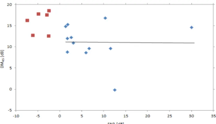
Fig. 15. Detection margin to 4.5σ versu detector with 5 s decision time. The data p were created by adding the background n shift to the training and testing signals. T margin above 20 dB are omitted and a least the raw data points (diamonds) is included.
As a final demonstration of the we use knowledge of the injectio detection measure as the difference background model log probabilit detector are shown in figure 16. Al variations before injection in one o a high value of σ and conseque detection margin.
us SNR for the background model points at negative SNR (squares) noise vector with arbitrary phase Three data points with detection t squares fit of a linear function to
ncy on SNR found from ever, since the spread in is
that the practical limit of few dB below zero. By e detector from 1 s to 5 s, he calculation of (5), the hown in figure 15. Here ative margin appears. This
noise variations observed W1 signals, yielding a high
us SNR for the background model points at negative SNR (squares) noise vector with arbitrary phase Three data points with detection t squares fit of a linear function to
HMM detector capability, on noise and create a new e between the injection and ties. The results for this lso here, background noise of the SW1 signals yielded ently a point at negative
Fig. 16. Detection margin to 4.5σ versus SNR for the injection-background difference detector with 5 s decision time. The data points at negative SNR (squares) were created by adding the background noise vector with arbitrary phase shift to the training and testing signals. Three data points with detection margin above 20 dB are omitted and a least squares fit of a linear function to the raw data points (diamonds) is included.
VII. DISCUSSION
In a relatively small mechanical system designed for injection experiments, it is difficult to exclude the possibility that the injections are detected through vibrations propagated directly from the injection mechanism itself rather than through jet noise and sodium-water reaction noise from the leak as would be the case in a real system.
The interpretation of the proposed feature calculation method is not obvious as it includes addition of frequency and power spectral density deviation, with the number as scaling constant. It obviously generates a feature that is suitable for HMM+GMM combination, but development of schemes with a clearer physical interpretation are of interest.
Furthermore, when a signal is changing, it is not certain that the conditional probability of (5) will change as we expect. Basically, we expect the background noise probability to go down and the injection noise probability to go up at injection onset. An interesting counterexample is seen in figure 7, where the injection seems to start in one flow regime and then change to another regime, more similar to that of the training data. The result is that initially, both the background noise and the injection noise probabilities go down.
The uncertain magnitude of the model probability changes is seen in figures 14, 15 and 16 as the detection margins have a relatively large spread and that outliers occur for models with high variance. Also, the SNR estimation of (13) is problematic as an unknown amount of acoustic absorption seems to occur during injections. This raises a question of the confidence level of the detector. On the other hand; the simple output distribution of the detector signal shown in figure 12 and the weak dependency on SNR observed in figures 14-16 are still properties that are encouraging for future work on this type of detector.
Earlier results, primarily from [3] have often focused on the low SNR capability and have also reached impressive results such as detection down to less than -20 dB. For the proposed method it seems probable that a limit of around -17 dB could be reached with acceptable false alarm rate,
although with a decision time that might be somewhat too long. However, the fact that very few earlier works report estimates on SNR limit, detection time and false alarm rates together makes thorough method comparison difficult. Differences between best and worst case performance are also seldom mentioned. One important explanation for this lack of estimates is that real plant data are so few and that background and leak noises of a new plant are extremely difficult to predict.
VIII. CONCLUSIONS
By comparing the proposed method with the requirements listed in section I of this paper the following conclusions can be drawn:
Injection rates below 1 g/s are clearly detected in all recordings and the false alarm criterion can be met. However, the SNRs of the SOWART acoustic signals are higher than expected in a real system. Crude extrapolation of the results to lower SNR suggests that the false alarm rate criterion can be met also in a more realistic sound environment by increasing the detector decision time and/or crediting injection noise models. However, the confidence level of the method is an open question, as it is for other methods presented in the literature.
Given that the detector output is approximately Gaussian, that the method will be able to model several noise types, that signal energy changes can successfully be discarded and that the proposed feature calculation scheme yields promising results, also without a priori knowledge on the injection noise, the method seems worthy of further research and development. Such R&D should include improvement of the feature calculation scheme, validation of the method at low SNR and further investigation of the relation between the feature calculation scheme, model size and performance of the detector.
ACKNOWLEDGMENTS
The authors express their sincere gratitude to the Director of IGCAR for his encouragement throughout the CEA-IGCAR collaborative program and to the staff members of the Fast Reactor Technology Group of IGCAR for their support in carrying out the SOWART experiments.
We also wish to thank Pierre-Augustin Grivelet of RMS Signal & Innovation for interesting and valuable discussions on the ALD problem.
REFERENCES
[1] Generation IV International Forum, “Generation IV Goals”, https://www.gen-4.org/gif/jcms/c_40472/technology-goals, Date of latest access: 2015-03-18
[2] J. Voss, P.J. Thomas and J.P. Girard, “Review of the Common European R & D Programme on Acoustic Leak Detection for Steam Generators”, IAEA Specialists’ Meeting on Steam Generators: Acoustic Detection of In-Sodium Water Leaks, Aix-en-Provence, 1 - 3 October, 1990
[3] International Atomic Energy Agency, “Acoustic signal processing for the detection of sodium boiling or sodium-water reaction in LMFRs”, IAEA-TECDOC-946, 1997
[4] N. Matta, Y. Vandenboomgaerde and J. Arlat, “Supervison and Safety of Complex Systems”, John Wiley & Sons, Inc., 2012, ISBN: 978-1-84821-413-2
[5] L. R. Rabiner, “A tutorial on hidden Markov models and selected applications in speech recognition”, Proceedings of the IEEE, Vol. 77, No. 2, pp. 257-285, 1989
[6] A. Leijon, “Pattern recognition - fundamental theory and exercise problems”, KTH Electrical Engineering, 2010
[7] P.D Welch, “The use of fast fourier transform for the estimation of power spectra: A method based on time averaging over short modified periodograms”, IEEE Transactions on Audio Electroacoustics, Vol. AU-15, pp.70-73, 1967
[8] G.S. Srinivasan, O.P. Singh and R. Prabhakar, “Leak noise detection and characterisation using statistical features”, Annals of Nuclear Energy, Vol. 27, pp. 329-343, 2000
[9] A. Riber Marklund and F. Michel, “Application of a new passive acoustic leak detection approach to recordings from the Dounreay prototype fast reactor”, submitted for publication
[10] S. Kishore, A. Ashok Kumar, S. Chandramouli, B.K. Nashine, K.K. Rajan, P. Kalyanasundaram, S.C. Chetal, “An experimental study on impingement wastage of Mod 9Cr 1 Mo steel due to sodium water reaction”, Nuclear Engineering and Design, Vol. 243, pp. 49-55, 2012