Large-Eddy Simulation of thermal striping in WAJECO and PLAJEST experiments with TrioCFD

HAL Id: cea-02509247

https://hal-cea.archives-ouvertes.fr/cea-02509247

HAL is a multi-disciplinary open access archive for the deposit and dissemination of sci-entific research documents, whether they are pub-lished or not. The documents may come from teaching and research institutions in France or abroad, or from public or private research centers.

L’archive ouverte pluridisciplinaire HAL, est destinée au dépôt et à la diffusion de documents scientifiques de niveau recherche, publiés ou non, émanant des établissements d’enseignement et de recherche français ou étrangers, des laboratoires publics ou privés.

Large-Eddy Simulation of thermal striping in WAJECO

and PLAJEST experiments with TrioCFD

P.-E. Angeli

To cite this version:

P.-E. Angeli. Large-Eddy Simulation of thermal striping in WAJECO and PLAJEST experiments with TrioCFD. NURETH 16 - 16th International Topical Meeting on Nuclear Reactor Thermalhydraulics, Aug 2015, Chicago, United States. �cea-02509247�

LARGE-EDDY SIMULATION OF THERMAL STRIPING IN WAJECO

AND PLAJEST EXPERIMENTS WITH TRIOCFD

Pierre-Emmanuel ANGELI

CEA-SACLAY, DEN/SAC/DANS/DM2S/STMF/LMSF, F-91191 Gif-sur-Yvette, France

pierre-emmanuel.angeli@cea.fr

ABSTRACT

This benchmark exercise is being performed under the auspices of an international collaboration on thermal hydraulics for sodium-cooled fast reactor development with participation from the Japan Atomic Energy Agency (JAEA), the U.S. Department of Energy (DOE), and the French Commissariat à l'Énergie Atomique et aux Énergies Alternatives (CEA). It is based on experiments performed to study the effects of thermal striping where three differentially heated jets mix inside a cavity. They were carried out either in water or in liquid sodium and velocity and temperature data were provided. The object of this paper is to predict numerically the results of these experiments and make comparisons with available measured data. The numerical simulations are led using the TrioCFD simulation code of the CEA. The Large-Eddy Simulation model is applied for the analyses. A computational domain reproducing the test sections is created. The discretization of the equations is based on unstructured staggered meshes and the resolution on a finite-volume approach. Coupled heat transfer between fluid and a metal test plate is considered. Overall, the numerical results achieve a good agreement with the experiments as well for the time-averaged fields as for the power spectrum densities of temperature fluctuations inside the fluid and the structure. A near-wall mesh refinement provides an obvious improvement of the accuracy of predicted temperature fluctuations.

KEYWORDS Jet mixing, thermal striping, turbulence, Large-Eddy Simulation, TrioCFD, Trio_U

1. INTRODUCTION

Thermal striping is the phenomenon of random temperature fluctuations resulting from the mixing of two non-isothermal streams. These fluctuations lead to high frequency thermal fatigue and crack appearance in the adjoining structures, especially with liquid metal coolant of high heat transfer coefficient such as sodium. Thus the study and limitation of this phenomenon is critical in the nuclear reactors safety domain. Thermal striping can occur at the core outlet of liquid metal cooled fast reactors [1][2], and has been the subject of various studies since the 1980s [3][4][5]. Experiments were performed to investigate the specificity of sodium in axial jets mixing compared to air jets [6][7]. Two test sections with three mixing jets were designed to estimate thermal striping phenomena. The water experiment called WAJECO [8][9][10] evaluated the mixing process along the jets. The liquid sodium experiment called PLAJEST for “PLAner triple parallel JEts Sodium experimenT” [11] examined the intensity of the attenuation process of temperature fluctuation from the fluid to a metal test plate set along the flow. Thereafter a metal test plate was also added in WAJECO leading to comparative results between water and sodium for the transfer characteristics of temperature fluctuations from fluid to structure [12][13].

The present study is carried out in the frame of a benchmark exercise associating the Japan Atomic Energy Agency (JAEA), the U.S. Department of Energy (DOE), and the French Commissariat à l'Énergie Atomique et aux Énergies Alternatives (CEA). It proposes a numerical analysis of WAJECO and

PLAJEST experiments based on computational fluid dynamics. The main objective is to provide thermal-hydraulic simulations of the three parallel jets mixing and comparisons with experimental data. JAEA previously used the CEA simulation tool TrioCFD to perform numerical simulations [14]. They employed a Large-Eddy model, a staggered finite-difference based discretization with a structured mesh, and considered the half-domain through the help of a symmetry condition. They found a good agreement with experimental data in wall-resolved mesh case but an underestimation of heat transfer in coarse mesh case. In the present study, Large-Eddy Simulations (LES) of WAJECO and PLAJEST experiments were performed using the TrioCFD software. The resolution is based on a staggered finite volume approach on unstructured meshes. The first section is dedicated to the overview of aforementioned experiments. Next section presents the outline of the numerical study and the comparison of calculated results with the experimental data.

2. OUTLINE OF WAJECO AND PLAJEST EXPERIMENTS

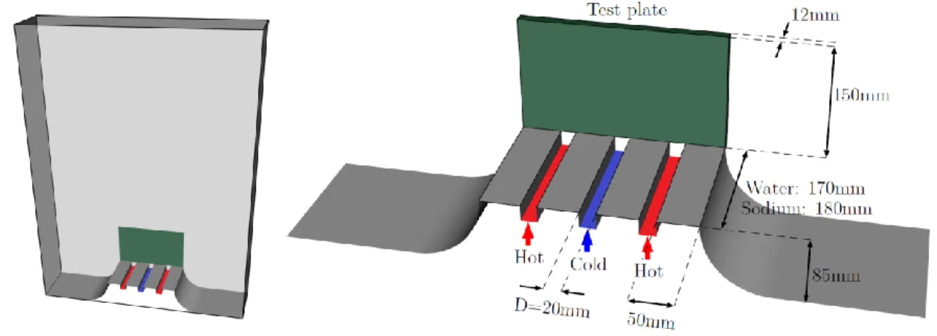
Figure 1 shows the experimental WAJECO and PLAJEST facilities. Both test sections are very similar. They consist of tanks limited by vertical partition plates and a curved metal bottom including a raised flat part. Three nozzle outlets with a rectangular cross section are designed on this part. Their depth is 180 mm in PLAJEST and 170 mm in WAJECO, and their width is 20 mm. A metal test plate made of stainless steel (SS316) is placed along one side wall to examine temperature fluctuations in the structure.

Figure 1. Experimental test section.

The water or sodium jets are configured as one cold stream vertically flowing out from the center nozzle and two hot streams vertically flowing out from side nozzles. The velocity and temperature of the cold jet (resp. hot jets) are called Vc and Tc (resp. Vh and Th). Several conditions are considered and detailed in

Table I. The corresponding cases will be referred to as A1, A2 and B1. Characteristic values related to mixing are introduced to be used later in the paper for nondimensionalization of the experimental and simulated data. The mean velocity, temperature difference between cold and hot jets, and mixed-mean temperature are respectively calculated as follows:

(1)

(3)

The Reynolds number is calculated from the mean velocity Vm and the nozzle width D:

(4)

The Reynolds number values are about 15,000 for PLAJEST and 26,000 for WAJECO. Table I. Summary of experimental conditions.

Outer-slits Center-slits Mixing characteristics Facility name Case Vh

(m.s-1) Th (°C) Vc (m.s-1) Tc (°C) Vm (m.s-1) Tm (°C) ΔT (°C) PLAJEST (sodium) A1 _B1 0.51 _0.51 347.5 _349.8 0.51 _0.32 304.5 ₃₁₁ 0.51 _{0.45 340.5} 333.2 _38.8 43 WAJECO (water) A2 0.48 40.3 0.48 32 0.48 37.5 8.3 The velocity field is captured by Particle Image Velocimetry (PIV) only in the water experiment. Since the liquid sodium is an opaque fluid, no velocity data can be measured in PLAJEST. For both experiments the temperature in the mixing area and the thermal exchange near the adjacent steel plate are measured by movable thermocouples. In order to investigate the temperature fluctuations inside the structure, thermocouples are installed in the plate. The interval between two temperature measurements in fluid is 0.01 second for both WAJECO and PLAJEST during respectively 42 and 200 seconds. In solid the measurements are done every 0.1 second during 200 seconds. After performing the water and the sodium experiments, JAEA provided numerous measurements to the benchmark participants for comparisons with the simulations. The available data are given in the form of time-averaged velocity, temperature and temperature fluctuation intensity profiles at typical positions in fluid and structure, as well as instantaneous temperature trends useful for spectral analysis.

3. NUMERICAL STUDY

3.1. Outline of the simulation code

The numerical simulation tool TrioCFD (called Trio_U up to 2015 [15][16]) of the Nuclear Energy Division of the CEA is employed to lead the calculations of the benchmark. TrioCFD is an object oriented and staggered finite volume based CFD code mostly dedicated to scientific and industrial applications related to the nuclear industry [17][18][19]. It embraces a variety of numerical methods, temporal and spatial discretizations, physical models and includes massive parallelism. TrioCFD is being permanently improved and validated within the CEA laboratory involved in the benchmark exercise. It is employed to perform analyses of turbulent flows and heat transfers in portions of nuclear facilities. The capability of coupled heat transfer between a fluid domain and a solid domain is available. For these reasons TrioCFD is expected to constitute an appropriate tool to investigate the jet mixing and thermal striping phenomena of the WAJECO and PLAJEST experiments. In 2015 TrioCFD has become an open-source software under the BSD license.

3.2. Computational domain and mesh characteristics

The TrioCFD models for the sodium and water experiments are very similar for both test sections. The x axis is the horizontal direction, y is the depth direction and z is the vertical direction. The lengths are respectively 770 mm, 180 mm (sodium case) or 170 (water case) and 1000 mm. The cavity is widely extended at the top to avoid numerical effects due to outlet (namely the interaction between the outgoing vortices and the outlet). The jet inlet is modeled by adding little channels in order that the velocity profiles are not flat on the nozzle outlets. No axial velocity fluctuation is added at these boundaries. The origin is set against the test plate at the center of the cold jet. The metal test plate is modeled only in the sodium case and is 12 mm thick, 250 mm wide and 160 mm tall. Thus in sodium case the solid domain corresponds to negative y values. The mesh of the calculation domain is divided into three regions: the mixing central area above the jet slits (which requires a fine mesh until twice the height of the test plane), and the upper and lateral areas (where a coarser mesh is acceptable). A near-wall correct prediction of temperature fluctuation intensity and thermal frequencies near the steel plate requires a specific mesh refinement in the interface region between the fluid and the structure. In a 5 mm layer, five prism layers are added and then divided into tetrahedra. The WAJECO mesh is very similar to the PLAJEST fluid mesh apart from a lack of near-wall mesh refinement. Some older PLAJEST results with an original non-refined mesh will also be given. The solid plate is meshed by extruding the surface mesh of the fluid/solid interface. The meshing process results in an unstructured mesh where the total tetrahedra number reaches 5,700,000 for the fluid domain and 700,000 for the solid domain. Parts of the mesh are visualized in Figure 2 and mesh details listed in Table II.

Table II. Mesh description.

PLAJEST A1-B1 WAJECO A2

Near-wall refinement Yes No

Fluid Number of cells 5,582,706 5,497,296

Characteristic mesh length 1.40 mm 1.41 mm

Solid Number of cells 720,432 -

Characteristic mesh length 0.9 mm -

3.3. Calculation parameters

The inlet velocities and temperatures of the jets are assigned to the uniform values from Table I. In the WAJECO case, the interaction between the fluid and the metal plate is modeled through a heat transfer coefficient. The vertical side surfaces are modeled as adiabatic non-slip walls. The effect of this choice on the mixing is expected to be weak because the domain was deliberately widened. The outlet condition at the top and at the front and back partition surfaces is an outflow with a uniform pressure.

The standard k-ε turbulence model was first put to the test and demonstrated its inability to capture the flow oscillations. The corresponding results are not presented in the present paper. The LES model is better suitable for jet calculations and is employed here. The subgrid scales are taken into account through the Wall-Adapting Local Eddy-viscosity model [20]. Mesh thickness and velocity conditions are such that the first calculation points for velocity and temperature are located at an average wall coordinate y+ around 14 (WAJECO) and 1.5 (PLAJEST) from the metal plate. The extremal y+ at the plate reaches respectively 55 and 35. Consequently the LES cannot be considered as wall-resolved. Then standard wall laws (valid from the viscous sublayer to the log-law region) are used to obtain correct velocity and temperature gradients at the first grid points.

The Navier-Stokes and thermal equations are solved through a finite-volume approach. The pressure is defined at the centers and vertices of computational cells and the velocity and temperature variables are located at the centers of the cell faces. A second order spatial scheme is used for both momentum and thermal convection operators. However in the upper corners of the domain a first-order upwind convection scheme is set in order to avoid numerical velocity divergence. A projection method is used to solve the velocity field. The pressure solver is based either on a Cholesky factorization (WAJECO), or on a preconditioned conjugate gradient method (PLAJEST).

In WAJECO case, the stability time steps associated to each equation are similar. The time discretization relies on a fully implicit Euler scheme with a Generalized Minimal RESidual (GMRES) method based solver. However in PLAJEST cases, the thermal stability time step (calculated as the harmonic mean of the diffusion time step and the convection time step) is much lower than the hydraulic stability time step. Thus a mixed implicit and explicit resolution is defined to speed up the calculations. The momentum equation is solved explicitly while the thermal equation is solved implicitly with a multiplicative coefficient for the thermal time step. The conduction time step inside the plate is much higher than the fluid time steps and is therefore not limiting in the coupled problem. Former PLAJEST simulations performed in CEA with TrioCFD compared fully implicit and explicit third-order Runge-Kutta temporal resolutions. They demonstrated that the ratio between the calculation times is close to 7 in favor of implicit method while both methods provide very similar results (Runge-Kutta results are not presented in the present paper). For this reason the fully implicit approach is preferred to the explicit Runge-Kutta. 3.4. Calculation performance

The meshes are divided into 256 zones in preparation for a parallel resolution. For the PLAJEST simulation, the number of degrees of freedom for velocity is 11 million and the order of the pressure matrix is 6.4 million. The simulations are launched on the CURIE and AIRAIN supercomputers, with respective peak performance of 200 Teraflop/s and 2 Petaflop/s. CURIE and AIRAIN belong to the CEA Very Large Computing Centre (TGCC) dedicated to High Performance Computing and opened to European scientists. Details related to calculation performance are summarized in Table III. As expected, the unstructured meshes lead to rather slow calculations and the computational cost is higher with the use of the computer AIRAIN. The time average range is assigned to a large value in order to obtain significant results. Nevertheless, the absence of wall coupling in the WAJECO case allows to stop the calculation earlier compared to PLAJEST cases. The time averaging is initiated after 10 physical seconds, when the transient effects are considered to have no more than a weak influence.

Table III. Summary of calculation performance.

PLAJEST A1 PLAJEST B1 WAJECO A2

Computer CURIE AIRAIN CURIE

CPUs 256 256 256

Final physical time (s) 200 200 100

Time average range (s) 10 – 200 10 – 200 10 – 100

Average time step (s) 0.000275 0.000274 0.000168

Time steps number 729,737 729,606 593,497

Effective resolution time 76 days 106 days 24 days

Figure 3 shows the evolution of temporal averages of velocity and temperature in the heart of the mixing zone for every calculation cases, according to subsequent definitions (5), (6) and (8). Smooth and low-varying values are reached at the final times indicating the convergence. In A2 case, it can be pointed out that convergence of thermal quantities is longer and not perfectly obtained. Long-term effects may affect the quality of convergence. Figure 3 also shows the temporal evolution of instantaneous velocity in B1 case, indicating that the flow establishment is shorter than 10 seconds.

Figure 3. Evolution of the normalized time-averaged quantities, in the mixing zone at the height z = 100 mm and at midpoint between front and back boundaries.

3.5. Numerical results

The time averages are computed from 10 seconds to avoid the initialization effects. The resulting average horizontal component of velocity, vertical component of velocity and temperature are respectively called Vx, Vz and T. In each case these quantities are made dimensionless with the mixing parameters of Table I,

namely

(5)

for velocity components and

(6)

for temperature. Thus the quantity

T

(7)

whereTis the instantaneous temperature fluctuation and N the size of the sample. It is normalized by

(8)

The Power Spectral Density (PSD) is computed from the Discrete Fourier Transform of time-depending variations of

T



) ( max * PSD PSD PSD frequency  ₍₉₎

The color scales in the contour plots are also normalized using previous definitions. The axes are normalized using the nozzle width D. The desired profiles are extracted using line probes for comparative plots.

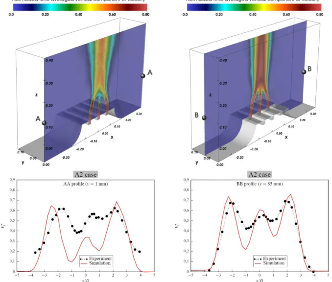
A2 results of velocity are first analyzed. On Figure 4 and Figure 5, the predicted velocity components in A2 case are plotted in vertical planes at midpoint between the front and back frontiers, and at close distance from the metal plate. The vertical velocity shows distinct peaks which are correctly reproduced, except the inaccurate location of the firs peak in comparison with experiment. The velocity variations between them are underestimated. The contrary occurs for horizontal velocity which is overestimated at the side peaks but is better predicted in the central area. In the simulation, the mean vertical flow is transformed into a mean horizontal movement in a larger way than in experiment.

Figure 4. Contours of time-averaged vertical velocity and associated profiles in A2 case. Overall the best agreement with the experiment is achieved along the center line, not along the near-wall line. For the A1-B1 results analyzed from now on, the same is true for the temperature distributions. In A1 case, the middle profiles are well reproduced with and without mesh refinement, as reported on Figure 6. Mesh refinement using a 5 mm layer of prisms has no obvious effect on the temperature results in iso-velocity case. In hetero-iso-velocity case, the asymmetry of the temperature near the steel plate is not captured by the LES contrary to the middle profile. The computed near-wall profile seems strongly symmetrical. It would probably be interesting to refine the mesh near the wall in B1 simulation to determine whether the effect would be more significant than in A1 case. It can also be suspected that the precision of spatial discretization schemes (of second order here) is insufficient. However the temperature levels are well predicted.

Figure 5. Contours of time-averaged horizontal velocity and associated profiles in A2 case. Figure 7 shows the distribution of temperature fluctuation intensity in A1 and B1 cases. It highlights a variability of results with regards to mesh refinement. In A1 case, the near-wall profiles are quite different but none reproduces correctly both side peaks. For the middle line, the slight asymmetry is captured only with the refined mesh, but the TFI is still a little overestimated. In B1 case, the variation of TFI are correctly predicted but distinctly overestimated for the center profile. Thus in every cases the instantaneous temperature values are more dispersed, which is interpreted as a reduced mixing compared to experiment.

Figure 8 compares the LES predictions for the decay of temperature fluctuation intensity with the normal distance from the metal plate surface. The profile C-C plotted in the figure is located at the height of 100 mm from the jet nozzles. A correct estimation of the decay of temperature fluctuation intensity is essential since it is in major part responsible for the thermal fatigue of the metal plate. There is a global good agreement for both meshes. In the near-wall region, the decay is underestimated at the closest experimental point from the wall in fluid side. However the mesh coarseness has a visible influence. The mesh refinement improves the result for the closest point but still seems insufficient.

Figure 7. Contours of time-averaged temperature fluctuation intensity in A1 case and associated profiles in A1-B1 cases.

Figure 8. Decay of time average temperature fluctuation intensity in normal direction to wall surface in case A1.

Power Spectral Densities are performed from the temperature time trends at different locations in the fluid and the solid. The PSD are compared to experimental data in Figure 9, after computing the convolution with the window filter in order to reduce the numerical noise.

Figure 9. Normalized power spectral densities of temperature at different locations in A1-A2 cases.

The PSD represents the response of the solid to the thermal excitation at its interface with the fluid. The PSD in solid in A1 case shows a greater attenuation and dispersion of the signal compared to experiment. Nevertheless, the refined mesh predicts well the predominant frequency of approximately 2-3 Hz while

the original mesh does not. In fluid the decay of power spectral densities is remarkably predicted, especially at the middle point. No real improvement is observed with the refined mesh. The actual number of computational nodes after refinement in fluid seems convenient for an accurate calculation of the thermal excitation near the plate. However the solid mesh should also be refined for a better prediction of the thermal fatigue modes of the metal plate.

4. CONCLUSIONS

This paper presented LES predictions for WAJECO and PLAJEST experiments using the TrioCFD software. Iso and hetero-velocity conditions were simulated according to given experimental jets parameters in order to evaluate the thermal fatigue on a stainless metal plate. Numerical results showed a good agreement with sodium and water experiments in most cases. The influence of a near-wall mesh refinement was investigated. Temperature and temperature fluctuation intensity are the most important quantities for this thermal fatigue study and their distributions were found to achieve the best agreements with the experimental results, while fluid velocity in the water case is on the whole underestimated. Near the wall, the mesh refinement using prism layers has positive consequences and improves most results. The thermal excitation is well estimated. However, the solid mesh remains too coarse to get a satisfactory representation of the metal plate response to the interfacial thermal excitation. The numerical study presented in the present paper confirms the relevance of the LES model in the context of thermal striping study for sodium nuclear reactors. They also bring overall the expected results to the benchmark exercise. Finally, they demonstrate the capability of the TrioCFD code to produce satisfactory results for such phenomena.

ACKNOWLEDGEMENTS

The author is grateful to JAEA for providing the experimental data. REFERENCES

[1] D. S. Wood, “Proposal for design against thermal striping”, Nucl. Energy, 19 (6), pp. 433-437 (1980).

[2] J. E. Brunings, “LMFBR thermal-striping evaluation”, Interim report, Research Project 1704-11, prepared by Rockwell International Energy Systems Group, EPRI-NP-2672 (1982).

[3] C. Betts, C. Bourman and N. Sheriff, “Thermal Striping in Liquid Metal Cooled Fast Breeder Reactors”, NURETH-2, Vol.2, pp. 1292-1301 (1983).

[4] S. Moriya, S. Ushijima, N. Tanaka, S. Adachi and I. Ohshima, “Prediction of Thermal Striping in Reactors”, Int. Conf. Fast Reactors and Related Fuel Cycles, Vol.1, pp. 10.6.1-10.6.10 (1991). [5] Tokuhiro, N. Kimura, J. Kobayashi and H. Miyakoshi, “An investigation on convective mixing of

two buoyant, quasi-planar jets with a non-buoyant jet in-between by ultrasound Doppler velocimetry”, ICONE-6, ICONE-6058 (1998).

[6] D. Tenchine and H. Y. Nam, “Thermal hydraulics of co-axial sodium jets”, Am. Inst. Chem. Engrs. Symp. Ser., 83 (257), pp. 151-156 (1987).

[7] D. Tenchine and J. P. Moro, “Experimental and numerical study of coaxial jets”, NURETH-8, Vol. 3, pp. 1381-1387 (1997).

[8] Tokuhiro, N. Kimura and H. Miyakoshi, “An experimental investigation on thermal striping. Part I: Mixing of a vertical jet with two buoyant heated jets as measured by ultrasound Doppler velocimetry”, NURETH-8, Vol. 3, pp. 1712-1723 (1997).

[9] Tokuhiro and N. Kimura, “An experimental investigation on thermal striping. Mixing phenomena of a vertical non-buoyant jet with two adjacent buoyant jets as measured by ultrasound Doppler velocimetry”, Nucl. Eng. Des., 188, pp. 49-73 (1999).

[10] N. Kimura, A. Tokuhiro and H. Miyakoshi, “An experimental investigation on thermal striping. Part II: Heat transfer and temperature measurement results”, NURETH-8, Vol. 3, pp. 1724-1734 (1997).

[11] N. Kimura, H. Miyakoshi and H. Kamide, “Experimental Investigation on Transfer Characteristics of Temperature Fluctuation from Liquid Sodium to Wall in Parallel Triple-Jet”, Int. J. Heat and Mass Transfer, 50, pp. 2024-2036, 2007.

[12] N. Kimura, H. Miyakoshi, H. Ogawa, H. Kamide, Y. Miyake and K. Nagasawa, “Study on Convective Mixing Phenomena in Parallel Triple-Jet along Wall - Comparison of Temperature Fluctuation Characteristics between Sodium and Water -”, NURETH-11, Paper: 427, Avignon, France, October 2-6 (2005).

[13] N. Kimura, H. Kamide, P. Emonot and K. Nagasawa, “Study on Thermal Striping Phenomena in Triple-Parallel Jet - Transfer Characteristics of Temperature Fluctuation in Sodium and Water based on Conjugated Numerical Simulation -”, NUTHOS-7, Seoul, Korea, October 5-9 (2008). [14] N. Kimura, H. Kamide, P. Emonot and K. Nagasawa, “Study on Thermal Striping Phenomena in

Triple-Parallel Jet - Investigation on Non-Stationary Heat Transfer Characteristics Based on Numerical Simulation -”, NURETH-12, Log Number: 117, Pittsburgh, Pennsylvania, U.S.A., September 30 - October 4 (2007).

[15] CEA/DEN/DANS/DM2S/STMF/LMSF, Trio_U User’s Manual, v1.7.0 (2014).

[16] P.-E. Angeli, U. Bieder and G. Fauchet, “Overview of the TrioCFD code: main features, V&V procedures and typical applications to nuclear engineering”, Proceedings of 16th International Topical Meeting on Nuclear Reactor Thermal Hydraulics (NURETH-16), Chicago, USA (September 2015).

[17] U. Bieder and E. Graffard, Qualification of the CFD code Trio_U for full scale reactor applications, Nucl. Eng. Des., 238 (3), pp. 671-679 (2007).

[18] U. Bieder, F. Falk and G. Fauchet, LES analysis of the flow in a simplified PWR assembly with mixing Grid, Prog. Nucl. Energy, 75, pp. 15-24 (2014).

[19] U. Bieder, F. Falk and G. Fauchet, CFD analysis of the flow in the near wake of a generic PWR mixing grid, Ann. Nucl. Energy (2014).

[20] F. Nicoud and F. Ducros, Subgrid-scale stress modelling based on the square of the velocity gradient tensor, Flow Turb. Comb., 62, pp. 183-200 (1999).