HAL Id: inria-00591035
https://hal.inria.fr/inria-00591035
Submitted on 6 May 2011
HAL is a multi-disciplinary open access
archive for the deposit and dissemination of
sci-entific research documents, whether they are
pub-lished or not. The documents may come from
teaching and research institutions in France or
abroad, or from public or private research centers.
L’archive ouverte pluridisciplinaire HAL, est
destinée au dépôt et à la diffusion de documents
scientifiques de niveau recherche, publiés ou non,
émanant des établissements d’enseignement et de
recherche français ou étrangers, des laboratoires
publics ou privés.
Two constrained formulations for deblurring poisson
noisy images
Mikael Carlavan, Laure Blanc-Féraud
To cite this version:
Mikael Carlavan, Laure Blanc-Féraud. Two constrained formulations for deblurring poisson noisy
im-ages. IEEE International Conference on Image Processing, 2011, Brussels, Belgium. �inria-00591035�
TWO CONSTRAINED FORMULATIONS FOR DEBLURRING POISSON NOISY IMAGES
Mikael Carlavan and Laure Blanc-F´eraud
ARIANA joint research group INRIA/I3S/UNSA
2004 route des Lucioles, 06902 Sophia-Antipolis, France
{Mikael.Carlavan, Laure.Blanc Feraud}@inria.fr
ABSTRACT
Deblurring noisy Poisson images has recently been subject of an in-creasingly amount of works in many areas such as astronomy or bi-ological imaging. Several methods have promoted explicit prior on the solution to regularize the ill-posed inverse problem and to im-prove the quality of the image. In each of these methods, a regu-larizing parameter is introduced to control the weight of the prior. Unfortunately, this regularizing parameter has to be manually set such that it gives the best qualitative results. To tackle this issue, we present in this paper two constrained formulations for the Poisson deconvolution problem, derived from recent advances in regulariz-ing parameter estimation for Poisson noise. We first show how to improve the accuracy of these estimators and how to link these esti-mators to constrained formulations. We then propose an algorithm to solve the resulting optimization problems and detail how to per-form the projections on the constraints. Results on real and synthetic data are presented.
Index Terms— Poisson deconvolution, discrepancy principle, constrained convex optimization.
1. INTRODUCTION
Deblurring images corrupted by Poisson noise is a challenging pro-cess which has devoted much research in many applications such as astronomical or biological imaging. If we consider a discrete version of a scene x∈ Rn(n being the number of pixels of the image)
ob-served as an image y∈ Rn
through an optical system with a Point Spread Function (PSF)h and corrupted by a Poisson noise process P, then the image formation model can be written as:
y= P(Hx + b), (1) where H: Rn
→ Rn
stands for the matrix notation of the convo-lution of the PSFh (we assume moreover Hx ≥ 0 ∀x ≥ 0) and b∈ Rn
, b ≥ 0 is a known constant background.
Using a bayesian approach, we want to retrieve the image x which maximizes the likelihood probability of (1). This probability can be expressed as: p(y|x) = n−1 Y i=0 „ [(Hx + b)y ]iexp [− (Hx + b)]i yi! « . (2) Maximizing (2) with respect to x is equivalent to minimize − log p(y|x) that is to minimize:
JL(x, y) = 1T(Hx + b) − yTlog(Hx + b), (3)
This research work has been funded by the ANR DetecFine. The authors gratefully acknowledge Pierre Weiss for several interesting discussions.
A part of this work has been submitted to IEEE Transactions on Image Processing.
where 1 stands for an-size vector whose components are all equal to1.
As discussed previously, many works promote the introduction of explicit prior on the solution to regularize the ill-posed inverse prob-lem. Maximizing the a posteriori probabilityp(x|y) = p(y|x)p(x)p(y),
where p(x) is the prior model on the object given by p(x) = α exp[−τJR(x)] (α is a normalization constant and JRis the
regu-larizing term), is equivalent to solve: x∗= arg min J(x, y) := J
L(x, y) + τ JR(x)
subject to x∈ Rn ,
(4)
τ being the regularizing parameter. The regularizing term can often be written asJR(x) = kWxk1, where W: Rn → Rp(p ≥ n)
is a linear transform which promotes the regularity of the image x in some domain. Common transforms are gradient operator giving Total Variation (TV) [1] and wavelet frame transforms ([2, 3] and references therein). Therefore the problem of deblurring Poisson noisy images can be written as:
x∗= arg min 1T (Hx + b) − yT log(Hx + b) + τ kWxk1 subject to x∈ Rn , x ≥ 0 . (5) The function to minimize is a closed convex function and strictly convex if yi> 0 and if the intersection of the null spaces of JLand
JRis zero [4].
In most of the deconvolution methods proposed in the literature, the regularizing parameterτ has to be chosen such that it gives the best visual results. However, the interpretation of an image may be difficult in biology for example, specially when one use priors which could introduce artifacts. To overcome this problem, some authors proposed estimators of the distance of the restored image to the real unknown image x [2, 5, 6, 7]. For example, several meth-ods based on Stein’s principle have been proposed to minimize (in one instance) the Mean Square Error (MSE) in the case of Pois-son noise [5]. However, these methods require the solution of the restoration algorithm to be expressed in closed-form and consist, most of the time, in a shrinkage of some wavelet coefficients. Con-sequently, the deconvolution process is rarely included in these tech-niques. Some authors have proposed non-linear algorithms as (5) to solve the restoration problem and to select the regularizing parame-ter using discrepancy principles which state that the distance of the restored image to the observation should be equal to the amount of noise [6, 7]. This implies however to run the restoration algorithm several times to find a “good” value of the regularizing parameterτ (that is, which verifies this principle). For this reason, we propose in the next section to solve the problem of deblurring and denoising Poisson noisy images using two new constrained formulations which avoid the iterative computation of the solution for different values of the regularizing parameter.
2. CONSTRAINED FORMULATIONS 2.1. Gaussian approximation revisited
To the best of our knowledge, constrained formulations for Poisson noisy deblurring have been proposed only using a Gaussian approx-imation. More precisely, the Poisson noise in (1) is often approxi-mated as an additive Gaussian noise with mean0 and multidimen-sional variance y [8]. If we set [6]:
r= (Hx − (y − b)) /√y, (6) then r is a Gaussian random variable with mean0 and variance I (the n-size identity matrix). In this case, a standard result gives krk2
2 ∼
χ2(n), where χ2(n) is the chi-square distribution with n degree of freedom which has a mean equal ton. Therefore:
E`krk22´ = n. (7)
Then a restoration algorithm in its constrained formulation can be written as: x∗= arg min kWxk 1 subject to k (Hx − (y − b)) /√yk2 2≤ n x∈ Rn , x ≥ 0 . (8)
However, a closer calculation of (7) can be made. As we deal with Poisson data, we have that, with no background, the image formation model writes y= P(Hx). Thus for every pixel xiinside a centered
window (of the size of the kernel of the PSF) containing only0 val-ued pixels, we can write that[P(Hx)]i = 0. Consequently, from
(6)(r)iis a Gaussian random variable with mean0 but variance 0. It seems thus more accurate to write that r is a Gaussian random variable with mean0 but variance Σ with:
Σ = ( 1 if yi> 0, 0 otherwise . (9) Then: krk22∼ χ2(m) with m = #{yi, yi> 0}, (10) and (8) becomes: x∗= arg min kWxk 1 subject to k (Hx − (y − b)) /√yk2 2≤ m x∈ Rn , x ≥ 0 . (11)
2.2. Poisson constrained formulation
Even if the previous formulation avoids to manually select a regular-izing parameter, it does not handle the Poisson noise statistics prop-erly. For this reason, from (5) we propose the following constrained formulation: arg min kWxk1 subject to Υy(Hx + b) ≤ α x∈ Rn , x ≥ 0 , (12) with: Υy(x) = 1 T (x) − yTlog(x) + yT log(y) − 1Ty. (13) In that case, the estimation ofα comes from the recent advances of [7] which introduced a discrepancy principle for Poisson data. The work of [7] is based from [9] in which the authors proposed, for
their numerical simulations, to select the regularizing parameter by means of a discrepancy principle, that is it should verify (using our notations):
Υy(Hx∗+ b) = Υy(Hx + b), (14)
where x∗denotes a solution of (5) for a givenτ and x is the true
object which verifies (1). However, in the case of real dataΥy(Hx+
b) remains unknown. [7] showed that Υy(Hx+b) can be estimated
using the following technique. First, they considered the function: f (Yλ) = 2 (λ − Yλlog(λ) + Yλlog(y) − Yλ) , (15)
where Yλis a Poisson random variable with meanλ. They showed
that, for largeλ:
E(f (Yλ)) = 1 + O
„ 1 λ
«
. (16) In the case of deconvolution, we have y= P(Hx + b) and thus y is a Poisson random variable with mean Hx+ b. Therefore:
E(Υy(Hx + b)) ≃
n
2. (17) So, from this statement [7] proposed to select the regularizing pa-rameterτ such that the solution x∗of the optimization problem (5)
verifies:
Υy(Hx∗+ b) ≃
n
2. (18) Thus, we propose to write our restoration algorithm as:
x∗= arg min kWxk 1 subject to Υy(Hx + b) ≤ n 2 x∈ Rn , x ≥ 0 . (19)
Using the same remark as previously, we also propose a slight modi-fication of this constrained formulation. Back to (15), if we consider that0 log(0) = 0, then f (yλ) = 0 for λ = 0. In consequence, the
proposed constrained formulation of (5) writes: x∗= arg min kWxk 1 subject to Υy(Hx + b) ≤ m 2 x∈ Rn , x ≥ 0 , (20)
wherem is given by (10). Solving problems (11) and (20) is not trivial and we propose an algorithm in the next section to solve them.
3. ALTERNATING DIRECTION METHOD
The algorithm we propose to use to solve (11) and (20) is based on the Alternating Direction Method (ADM). The idea of the ADM method is to split the original variablex into several variables and then to minimize the augmented Lagrangian following each splitted variable. The ADM method has been recently proposed to solve the unconstrained formulation (5) in [4]. Its presentation is however be-yond the scope of this paper, and we refer the interested reader to [4] (and references therein). But this technique can also be used to solve our constrained Poissonian deconvolution problem, and we will di-rectly give the resulting algorithm.
The functions (11) and (20) to minimize in Rnare coercive, lower semi-continuous and the constraint sets are non-empty closed convex sets. Then, for each problem, a solution x∗exists and an estimate of
this solution can be computed by the algorithm 1. This algorithm in-troduces a relaxation parameterγ, which has to belong to ]0,√5+12 [
to ensure the convergence of the algorithm [10], andβ which is the parameter which controls the constraint. Theoritically, the algorithm converges for anyβ > 0, but the speed of convergence strongly de-pends on this parameter. For our expriments, we will setβ = 10 and γ = 1. Finally, ΠK is the orthogonal projection on the convex set
K defined by:
K =˘w ∈ Rn, wi> 0, k(w − y)/√yk22≤ m¯ . (21)
for the problem (11) and :
K =nw∈ Rn, wi> 0, Υy(w) ≤
m 2
o
. (22) for the problem (20). The orthogonal projection (21) can be seen as a projection on a weightedl2-ball and can be found in [11] for
example. So we do not detail any further the computation of this projection. We focus instead on the orthogonal projection (22) which is not obvious. Even if we can not give a closed-form solution of this projection, we propose an iterative scheme to solve it. We recall that the orthogonal projection problem is to find:
w∗= Π K(w0) = arg min 12kw − w0k22 subject to Υy(w) ≤ m 2 w∈ Rn . (23)
First notice that ifΥy(w0) ≤ m
2 then w∗= w0. Otherwise, there
existsδ ∈ ]0, +∞[ such that: w∗= arg min 1
2kw − w0k 2
2+ δΥy(w)
subject to w∈ Rn . (24)
From [12], we get that: w∗=1 2 » w0− δ + q (w0− δ)2+ 4δy – = Φ(δ). (25) The problem is thus to findδ such that Υy(Φ(δ)) ≤
m 2. Let us define: f (δ) := Υy(Φ(δ)) − m 2. (26) It can be shown thatf is a convex and decreasing function with respect toδ. In order to find the root of the function f , we propose to use a Newton method and we only need to findf′(δ). Simply remark that from the composition of functions, we have:
f′(δ) = 1 T 2 ( " δ − x0+ 2y p(x0− δ)2+ 4δy − 1 # " 1 − 2y x0− δ +p(x0− δ)2+ 4δy # ) . (27)
The resulting algorithm is then given in the algorithm 2. In all our simulations, we checked that 20 iterations of this scheme are more than enough to get a machine precision.
4. RESULTS
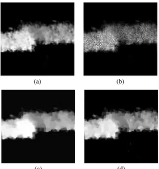
We compared the results obtained using the Poisson constrained for-mulation (20) and the ones obtained using the weighted Gaussian constrained formulation (11) with the TV regularization. Results on synthetic image are given on figure 1. On this image, the blur H is a7 × 7 Gaussian kernel. For low intensity images like the im-age (a) on the figure 1, the weighted Gaussan approximation is not efficient, and the results given by the Poisson formulation (20) are
Algorithm 1: ADM to solve (11) and (20) Data: Number of iterationsN ;
Starting points x0= y, λ01= 0, λ02= 0, λ03= 0;
Value of the parametersγ > 0 and β > 0;
Result: xNan estimated of the solution of (11) and (20). begin 1. s0= Hx0+ b 2. t0= Wx0 fork from 0 to N − 1 do 3. xk+1= max“xk+λ k 1 β , 0 ” 4. uk+1= ΠK “ sk+λ k 2 β ” 5. vk+1= sign“tk+λ k 3 β ” max“˛˛ ˛t k+λk3 β ˛ ˛ ˛ − 1 β, 0 ” 6. zk+1= xk+1−λ k 1 β + H∗“uk+1− b − λ k 2 β ” + W∗“vk+1−λ k 3 β ” 7. xk+1= (H∗H+ W∗W+ I)−1zk+1 8. sk+1= Hxk+1+ b 9. tk+1= Wxk+1 10. λk+11 = λk1+ βγxk+1 11. λk+1 2 = λ k 2+ βγsk+1 12. λk+13 = λk 3+ βγtk+1 end end
Algorithm 2: Newton method to solve (23) Data: Number of iterationsN ;
A starting pointδ0= 0;
Result: w∗an estimated of the solution of (23).
begin fork from 0 to N − 1 do Step 1. δk+1= δk −ff(δ′(δkk)) end w∗= 1 2 » w0− δN+ q (w0− δN)2+ 4δNy – end
clearly better (the image (d) on the figure 1 shows an improvement of 2.5dB). The Poisson formulation (20) may however be slightly outperformed by the the weighted Gaussian constrained formulation (11) on high intensity images for which the Poisson distribution is well approximated by a weighted Gaussian distribution (not shown here). Results on a real image are given on the figure 2. On this image, H is a confocal microscope PSF whose model is described in [1]. The image retrieved with the proposed formulation (image (d) on the figure 2) is less smoothed than the one retrieved with the weighted Gaussian approximation. We can distinguish more easily the details of the cells of the object.
5. CONCLUSION
We have studied the problem of deconvolution of images corrupted by blur and Poisson noise and have proposed two new constrained formulations derived from recent regularizing estimation techniques. We have shown that the accuracy of these estimators can be
im-(a) (b)
(c) (d)
Fig. 1. Results of constrained formulations (11) and (20) on a low synthetic intensity image. (a) is the original image, (b) is the blur and noisy observation (P SN R = 23.9 dB), (c) is the result with the weighted Gaussian constrained formulation (11) (P SN R = 28.0 dB) and (d) is the result with the Poisson constrained formulation (20) (P SN R = 30.5 dB). The original Gaussian constrained for-mulation (8) and the original Poisson constrained forfor-mulation (19) respectively giveP SN R = 22.8 dB and P SN R = 23.4 dB (im-ages not included here)
proved by taking into account the properties of the Poisson statistics of the noise, and that these estimators can also be used to write con-straint formulations which avoid the computational burden required by the regularizing parameter estimation in the unconstrained form. Finally, we have proposed an algorithm to solve the resulting opti-mization problems and their respective projections. A comparison of both formulations has been presented on synthetic and real data showing that the Poisson formulation is actually very promising for images with low intensity.
6. REFERENCES
[1] N. Dey, L. Blanc-F´eraud, C. Zimmer, Z. Kam, P. Roux, J. C. Olivo-Marin, and J. Zerubia, “Richardson-lucy algorithm with total variation regularization for 3d confocal microscope de-convolution,” Microscopy Research Technique, vol. 69, pp. 260–266, 2006.
[2] F.-X. Dup´e, J. Fadili, and J.-L. Starck, “A proximal iteration for deconvolving poisson noisy images using sparse represen-tations,” IEEE Transactions on Image Processing, vol. 18, no. 2, pp. 310–321, Feb. 2009.
[3] N. Pustelnik, C. Chaux, and J.-C. Pesquet, “Hybrid regulariza-tion for data restoraregulariza-tion in the presence of Poisson noise,” in 17th European Signal Processing Conference (EUSIPCO’09), Aug. 2009.
[4] M. A. T. Figueiredo and J. M. Bioucas-Dias, “Restoration of
(a) (b)
(c) (d)
Fig. 2. Results of constrained formulations (11) and (20) on a3D real biological image. (a) is the observed image (sample of mouse intestine), (b) is a zoom on the observation, (c) is the result with the weighted Gaussian constrained formulation (11) and (d) is the result with the Poisson constrained formulation (20)
poissonian images using alternating direction optimization,” Accepted to IEEE Transactions on Image Processing, Jan. 2010.
[5] F. Luisier, T. Blu, and M. Unser, “Image denoising in mixed poisson-gaussian noise,” IEEE Transactions on Image Pro-cessing, vol. 20, no. 3, pp. 696 –708, Mar. 2011.
[6] J. M. Bardsley and J. John Goldes, “Regularization parameter selection methods for ill-posed poisson maximum likelihood estimation,” Inverse Problems, vol. 25, no. 9, 2009.
[7] M. Bertero, P. Boccacci, G. Talenti, R. Zanella, and Zanni L., “A discrepancy principle for poisson data,” Inverse Problems, vol. 26, 2010.
[8] A. Grinvald and I. Z. Steinberg, “On the analysis of fluores-cence decay kinetics by the method of least-squares,” Analyti-cal Biochemistry, vol. 59, no. 2, pp. 583–598, 1974.
[9] T. Le, R. Chartrand, and T. J. Asaki, “A variational approach to reconstructing images corrupted by poisson noise,” J. Math. Imaging Vis., vol. 27, pp. 257–263, Apr. 2007.
[10] R. Glowinski, Numerical Methods for Nonlinear variation al Problems, Springer-Verlag, 1984.
[11] P. Weiss, L. Blanc-F´eraud, and G. Aubert, “Efficient schemes for total variation minimization under constraints in image pro-cessing,” SIAM journal on Scientific Computing, vol. 31, no. 3, pp. 2047–2080, 2009.
[12] P. L. Combettes and V. R. Wajs, “Signal recovery by proximal forward-backward splitting,” Multiscale Modeling & Simula-tion, vol. 4, no. 4, pp. 1168–1200, 2005.