HAL Id: cea-01485216
https://hal-cea.archives-ouvertes.fr/cea-01485216
Submitted on 8 Mar 2017
HAL is a multi-disciplinary open access
archive for the deposit and dissemination of
sci-entific research documents, whether they are
pub-lished or not. The documents may come from
teaching and research institutions in France or
abroad, or from public or private research centers.
L’archive ouverte pluridisciplinaire HAL, est
destinée au dépôt et à la diffusion de documents
scientifiques de niveau recherche, publiés ou non,
émanant des établissements d’enseignement et de
recherche français ou étrangers, des laboratoires
publics ou privés.
Turbulent drag in a rotating frame
Antoine Campagne, Nathanaël Machicoane, Basile Gallet, Pierre-Philippe
Cortet, Frédéric Moisy
To cite this version:
Antoine Campagne, Nathanaël Machicoane, Basile Gallet, Pierre-Philippe Cortet, Frédéric Moisy.
Turbulent drag in a rotating frame. Journal of Fluid Mechanics, Cambridge University Press (CUP),
2016, 794, �10.1017/jfm.2016.214�. �cea-01485216�
arXiv:1603.06484v1 [physics.flu-dyn] 21 Mar 2016
This draft was prepared using the LaTeX style file belonging to the Journal of Fluid Mechanics 1
Turbulent drag in a rotating frame
Antoine Campagne
1, Nathana¨
el Machicoane
1, Basile Gallet
2,
Pierre-Philippe Cortet
1, and Fr´
ed´
eric Moisy
11
Laboratoire FAST, CNRS, Univ. Paris-Sud, Universit´e Paris-Saclay, 91405 Orsay, France 2
Service de Physique de l’´Etat Condens´e, CEA, CNRS, Universit´e Paris-Saclay, CEA Saclay, 91191 Gif-sur-Yvette, France
(Received xx; revised xx; accepted xx)
What is the turbulent drag force experienced by an object moving in a rotating fluid? This open and fundamental question can be addressed by measuring the torque needed to drive an impeller at constant angular velocity ω in a water tank mounted on a platform rotating at a rate Ω. We report a dramatic reduction in drag as Ω increases, down to values as low as 12% of the non-rotating drag. At small Rossby number Ro = ω/Ω, the decrease in drag coefficient K follows the approximate scaling law K ∼ Ro, which is predicted in the framework of nonlinear inertial wave interactions and weak-turbulence theory. However, stereoscopic particle image velocimetry measurements indicate that this drag reduction rather originates from a weakening of the turbulence intensity in line with the two-dimensionalization of the large-scale flow.
1. Introduction
Determining the drag force on a moving object is a central question of turbulence research and the main goal of aerodynamics. A characteristic feature of turbulent flows is the “dissipation anomaly”: the drag force becomes independent of the fluid’s viscosity when the latter is low enough (Frisch 1995). A simple experiment highlighting this behavior consists in spinning an impeller of radius R and height h at constant angular velocity ω inside a tank filled with fluid of density ρ and kinematic viscosity ν: when the Reynolds number Re = R2ω/ν is large enough, the torque Γ required to drive the
impeller follows the ν-independent scaling Γ = KρR4hω2, where the dimensionless drag
coefficient K depends only on the shape of the impeller.
Here we consider the effect of global rotation at constant rate Ω on this fundamental experiment: how does the drag coefficient depend on the Rossby number Ro = ω/Ω? Global rotation is encountered in many industrial, geophysical and astrophysical flows. Rotating turbulence has therefore been studied intensively using experimental, theoret-ical and numertheoret-ical tools (Davidson 2013; Godeferd & Moisy 2015). For strong global rotation, the behavior of rotating turbulent flows may be summarized as follows: the large-scale flow structures tend to become invariant along the global rotation axis, in qualitative agreement with the Taylor-Proudman theorem (Greenspan 1968), while the remaining vertically dependent fluctuations can be described in terms of inertial waves that interact nonlinearly, together and with the 2D flow (Clark di Leoni et al. 2014; Yarom & Sharon 2014; Campagne et al. 2014, 2015; Alexakis 2015). Rotating turbulence is therefore intermediate between 2D and 3D turbulence; one naturally wonders how its energy dissipation rate compares to the laminar dissipation of 2D turbulence, or to the dissipation anomaly of 3D turbulence.
(a)
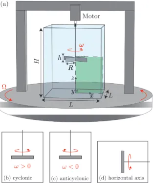
(b) cyclonic (c) anticyclonic (d) horizontal axis x x x y y z z Motor Ω ω ω ω L R R R h h L H ω>0 ω<0
Figure 1.Experimental setup. We measure the mean torque Γ developed by the motor driving an impeller at constant rotation rate ω in a water-filled tank mounted on a platform rotating at rate Ω (L = 45 cm, H = 55 cm, R = 12 cm, h = 3.2 cm). In (a), (b) and (c), the platform and the impeller rotate around the same axis (in the laboratory frame, the impeller spins at a rate ω + Ω). PIV measurements are performed in a vertical plane (green dashed region). In (d), the axis of the impeller is perpendicular to the global rotation axis of the platform.
turbulent dissipation. Indeed, torque measurements give access to the drag coefficient: K = Γ/(ρR4hω2) , (1.1)
i.e., to the normalized energy dissipation rate. We report on the behavior of K as a function of the Rossby number Ro, in the fully turbulent regime where K is independent of Re, for a rotation axis of the impeller either parallel or perpendicular to the global rotation axis.
2. Experimental setup
The experimental setup is sketched in figure 1(a). It consists of a parallelepipedic water-filled tank of height H = 55 cm and square base of side L = 45 cm. A brushless servo-motor drives a four-rectangular-blade impeller of radius R = 12 cm and height h = 3.2 cm at constant angular velocity ω between 20 and 400 rpm. The tank and the motor are mounted on a 2-meter-diameter platform rotating at constant rate Ω > 0 up to 30 rpm around the vertical axis. For each set of parameters (ω, Ω), we measure the time-averaged torque Γ developed by the motor driving the impeller. The maximum applied torque is Γm= 5 N m. We subtract the non-hydrodynamic torque, determined
for each value of ω by repeating the measurement using air instead of water. This non-hydrodynamic torque includes losses in the motor and in the o-ring seal through which
Turbulent drag in a rotating frame 3 100 101 102 103 10−1 100 Ω (rpm)
K
∞K
ω< 0 ω> 0 h. a.|Ro|
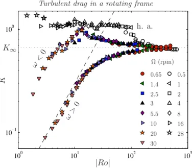
0.65 1.4 2.5 3 5.5 10 20 30 0.5 1 2 4 8 16 28Figure 2.Drag coefficient K = Γ/ρR4 hω2
as a function of the Rossby number |Ro| = |ω|/Ω. Color symbols: vertical-axis configuration, cyclonic and anticyclonic (figure 1b,c); Open symbols: horizontal-axis configuration (figure 1d). The horizontal dotted line is the drag coefficient for fully developed turbulence without rotation, K∞ = 0.67 ± 0.02. The tilted dashed line shows K ∝ Ro.
the shaft enters the tank. It is determined with a precision of ∆Γ = 50 mN m, allowing us to span a range of two orders of magnitude in hydrodynamic torque.
Two configurations are considered. In the first configuration, the impeller rotates around the vertical axis, either cyclonically (ω > 0, figure 1b) or anti-cyclonically (ω < 0, figure 1c); in the second configuration, the impeller rotates around a horizontal axis in the rotating frame (figure 1d). These configurations allow us to examine the two physically relevant situations of a driving velocity either normal or parallel to the global rotation axis. The vertical-axis configuration (figure 1b,c) bears some similarities with the Taylor-Couette flow between rotating cylinders, the key difference being that the flow is driven inertially: the Taylor-Couette geometry is well-suited to study the effect of global rotation on viscous friction near a smooth wall, while our experiment considers the turbulent drag due to the inertially driven flow.
3. Drag measurements
We first focus on the vertical-axis configuration. Figure 2 shows the drag coefficient (1.1) as a function of the Rossby number |Ro| = |ω|/Ω. K is related to the spatial distribution of energy dissipation rate per unit mass ǫ(x) = νh|∇u|2i
t through the
balance between input and dissipated power: Γ ω = ρV hǫix, where h it denotes a time
average and h ixthe space average over the volume V = L
2H of the tank. In the absence
of global rotation, because of the large Reynolds number of the flow (Re = 6.4 × 10⁴ to
6.7 × 10⁵), the drag coefficient is independent of Re, K
∞= 0.67 ± 0.02, in agreement with
the fully turbulent scaling law ǫ ∼ R3ω3/h. For nonzero global rotation Ω > 0, the drag
coefficient remains independent of Re, but it is now a function of the Rossby number: the high-Re data for Γ (ω, Ω) collapse onto two master branches when plotted as K vs. |Ro|, a cyclonic branch for ω > 0 and an anticyclonic branch for ω < 0.
−0.30 −0.15 0 0.15 0.3 0.4 0.8 1.2 0.65 1.4 2.5 3 5.5 10 20 30 0 Ω (rpm) K 1/Ro
Figure 3.The drag coefficient K departs from K∞approximately linearly in inverse Rossby number Ro−1
= Ω/ω, when the latter is small (same data as figure 2).
the two branches split symmetrically about K∞, with drag reduction for cyclonic motion
(Ro > 0) and drag enhancement for anticyclonic motion (Ro < 0). Such small departure from K∞ can be described through a regular expansion in Ro
−1= Ω/ω, assuming that
the weak Coriolis force can be accounted for perturbatively: writing the velocity field as u = u0+ Ro−1u1+ O(Ro−2), where u0 is the flow without global rotation, leads to
u1|−Ω= u1|Ω. The mean energy dissipation rate per unit mass is hǫix= νh|∇u0| 2i
x,t+
2νRo−1h∇u
0 · ∇u1ix,t+ O(Ro
−2), where h i
x,t denotes space and time average, and
νh|∇u0|2ix,tis the energy dissipation rate of the non-rotating flow. The drag coefficient
becomes
K K∞
= 1 + αRo−1+ O(Ro−2) , where α = 2h∇u0· ∇u1ix,t
h|∇u0|2ix,t
. (3.1) The sign of α can be inferred from the fact that global rotation tends to reduce the velocity gradients along the rotation axis. In the laboratory frame, and for fixed Ω > 0, the fluid spins faster for cyclonic rotation of the impeller (ω > 0) than for anticyclonic rotation (ω < 0). As a consequence, we expect lower vertical velocity gradients in the cyclonic case, i.e., α < 0, implying consistently a negative correlation between the perturbed vertical derivative ∂zu1 and ∂zu0 in equation (3.1). The data in figure 3 are in good
agreement with this prediction: the departure of K from K∞ is approximately linear in
Ro−1 for Ro−1∈ [−0.07; 0.07], which corresponds to the range |Ro| > 15 in figure 2.
We now discuss the regime Ro ≃ 1, which is probably the most interesting one: the cyclonic branch of figure 2 displays a dramatic drop in drag coefficient, with K reaching values as low as 12% of K∞ for the lowest Rossby numbers. This decrease
in drag with increasing Ω follows the approximate scaling law K ∼ Ro. A similar – although less pronounced – decrease in drag coefficient is observed for the anticyclonic branch. However, it is preceded by a dissipation peak at intermediate Ro: a maximum dimensionless drag Kpeak ≃ 1.5K∞ is achieved for Ropeak ≃ −12. Once again, this
difference between the two branches can be related to the effective global rotation of the fluid: the dissipation peak corresponds to anticyclonic impeller motion ω < 0 partly compensating the rotation Ω > 0 of the platform, so that the fluid has minimum global rotation in the laboratory frame. A similar peak of dissipation has been
Turbulent drag in a rotating frame 5 reported for counter-rotating Taylor-Couette flow, and corresponds to optimal transport of angular momentum between the two cylinders (Dubrulle et al. 2005; Van Gils et al. 2011; Paoletti & Lathrop 2011; Ostilla-M´onico et al. 2014). Such intermediate negative Rossby numbers also represent the most unstable configuration for vortices in rotating flows (Kloorsterziel & Van Heijst 1991; Mutabazi et al. 1992), which rapidly break down into highly-dissipative 3D structures. The Taylor-Couette dissipation peak can then be traced back to strong instabilities driving dissipative 3D flow structures. In a similar fashion, the PIV measurements described in section 4 indicate that highly-dissipative 3D flow structures are responsible for the dissipation peak of the present experiment (see figure 4c).
How to explain such a strong drag reduction for rapid global rotation? Two scenarios can be put forward. A first scenario relies on the modification of the energy transfers by the background rotation. In this approach, the velocity fluctuations are described in terms of propagating inertial waves, which disrupt the phase relation needed for efficient energy transfers (Cambon & Jacquin 1989). This scenario was first put forward in the context of magnetohydrodynamic turbulence (Iroshnikov 1964; Kraichnan 1965), and later applied to rapidly rotating turbulence (Zhou 1995; Smith et al. 1996). It predicts reduced energy transfers ǫ ≃ ǫ∞Ro
′
in the limit Ro′
≪ 1, where ǫ∞≃ u
′3/ℓ is the usual
(non-rotating) dissipation rate constructed on the turbulent velocity u′
and the energy-containing size ℓ, and Ro′
= u′
/2Ωℓ is the turbulent Rossby number. This result, which relies on dimensional analysis, can be made more quantitative in the framework of wave turbulence theory (Galtier 2003; Cambon et al. 2004; Nazarenko 2011). Even though the latter theory is valid for Ro′
≪ 1 only (to be compared to the lowest value Ro′
≃ 0.2 of the present study, see Table 1), the scaling law K ∼ Ro reported in figure 2 turns out to be in agreement with this prediction, if one assumes that u′
∼ Rω holds regardless of Ro.
Another explanation for the decrease in drag coefficient is partial two-dimensionalization. Indeed, the forcing geometry in the vertical-axis configuration (figure 1b,c) is compatible with the Taylor-Proudman theorem, which predicts for low Ro a purely 2D vertically invariant solution corresponding to solid-body rotation in the cylinder tangent to the impeller, at angular velocity ω in the rotating frame of the platform. This solution is valid for a perfect fluid only, which slips on the top and bottom boundaries. For a realistic viscous fluid, additional boundary layers and poloidal recirculations develop and coexist with the solid-body motion (Hide & Titman 1967; Greenspan 1968). As a matter of fact, for periodic boundary conditions and idealized vertically invariant forcing, it was recently proven that the high-Re flow settles in a purely 2D state for low enough Rossby number (Gallet 2015). For the experiment at stake here, the rapidly rotating flow can be thought of as a coexistence of this 2D asymptotic flow, together with weak 3D turbulent fluctuations, the intensity of which decreases as global rotation increases. The 2D flow dissipates very little energy, at a laminar rate, typically proportional to viscosity. Accordingly, energy dissipation is due to the 3D flow structures, the intensity of which decreases for decreasing Ro. We therefore expect a decrease in energy dissipation – and therefore in drag coefficient – for increasing global rotation rate.
4. Turbulent flow structure
To discriminate between the inertial-wave scenario and the partial two-dimensionalization one, we measure the velocity field using a stereoscopic PIV system mounted on the rotating platform. The field of view is vertical, illuminated by a laser sheet containing the axis of the impeller, and represents one quarter of the tank section, below the impeller
z 0 −H/2 z 0 −H/2 z 0 −H/2 x 0 L/2 x 0 L/2
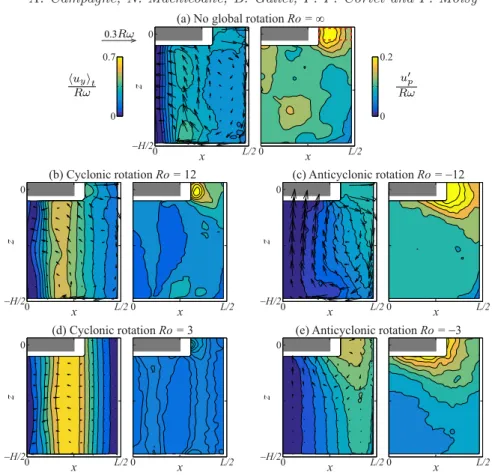
(a) No global rotation Ro = ∞
0 0.1 0.2 0 0.7 Rω t i y u h 0.3Rω z 0 −H/2 (c) Anticyclonic rotation Ro = −12 x 0 L/2 x 0 L/2 x 0 L/2 x 0 L/2 x 0 L/2 x 0 L/2 z 0 −H/2 x 0 L/2 x 0 L/2
(e) Anticyclonic rotation Ro = −3 (b) Cyclonic rotation Ro = 12 (d) Cyclonic rotation Ro = 3 Rω p ′ u 0 0.2 0 0.1 0.2
Figure 4.Time-averaged flow (left) and rms fluctuations of the poloidal flow (right), measured by stereoscopic PIV in the frame of the rotating platform. In the left panels, the color codes the toroidal (out-of-plane) velocity. (a), no background rotation (ω = 150 rpm, Ω = 0). (b,d), cyclonic background rotation (Ro = 12 and 3). The two-dimensionalization results in a gradual weakening of the poloidal flow upand a strengthening of the toroidal flow; at the largest global rotation (d), the fluid column below the impeller rotates rigidly at ω in the rotating frame, with weak turbulent fluctuations. (c,e), anticyclonic background rotation (Ro = −12 and −3). The peak dissipation at Ro ≃ −12 in figure 2 corresponds to the maximum poloidal recirculation and maximum turbulent fluctuations in the vicinity of the impeller (panel c).
Panel Ro = ω Ω Re = ωR2 ν Ro ′ = u ′ p 2Ωh Re ′ =u ′ ph ν (a) ∞ 2.3 × 10⁵ ∞ 7.2 × 10³ (b) 12 1.8 × 10⁵ 2.4 5.1 × 10³ (c) −12 1.8 × 10⁵ 3.3 7.2 × 10³ (d) 3 1.4 × 10⁵ 0.2 1.6 × 10³ (e) −3 1.4 × 10⁵ 0.7 4.4 × 10³
Table 1.Dimensionless numbers for the five panels of figure 4, based either on the control parameters or on the fluctuating poloidal velocity (inside the red-dashed domain of figure 4a).
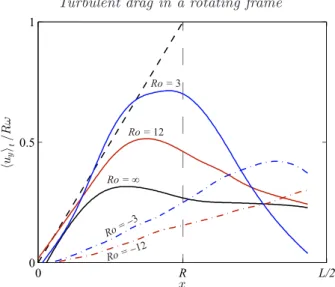
Turbulent drag in a rotating frame 7 Ro = ∞ Ro = 12 Ro = 3 Ro = −12 Ro = −3 R L/2 0 0 0.5 1 x huy it / R ω
Figure 5. Mean azimuthal (out-of-plane) velocity profile huyit, measured 200 mm below the propeller (z/H = −0.36), showing the strong two-dimensionalization of the flow for cyclonic background rotation (Ro > 0). The dashed line shows the Taylor-Proudman prediction huyit= ωx (solid-body rotation at angular velocity ω in the rotating frame).
(see figure 1a). Stereoscopic PIV measurements are achieved by two high-resolution cameras aimed at the measurement plane at an incidence angle of 45◦
, at a frame rate of 5 Hz.
In figure 4, we show the mean velocity field, and the standard deviation u′
p(x, z) of
the poloidal velocity, with and without global rotation. The non-rotating mean flow corresponds to a toroidal (out-of-plane) flow driven by the propeller, together with a strong poloidal (in-plane) recirculation. The flow displays 3D turbulence, the intensity of which is maximum at the edge of the impeller’s blades. In table 1, we provide values of the turbulent Reynolds and Rossby numbers based on the rms poloidal velocity in this flow region (red-dashed domain in figure 4a).
The non-rotating flow contrasts strongly with the rapidly rotating one measured for cy-clonic impeller motion: in line with the Taylor-Proudman theorem, the mean toroidal flow gradually tends to solid-body rotation at frequency ω inside the tangential cylinder, while the mean poloidal recirculation weakens as Ω increases. This two-dimensionalization is clearly visible in figure 5, which shows the mean azimuthal velocity profile well below the impeller (z/H = −0.36). Another consequence of the Taylor-Proudman theorem is a strong decrease of the 3D turbulent fluctuations for decreasing Rossby number, as can be seen on the right-hand panels of figure 4b,d: in the vicinity of the blades, i.e., inside the red-dashed domain sketched in figure 4a, both the poloidal and toroidal rms velocities strongly decrease for decreasing Rossby number (we show only the former), the ratio of the two being approximately 1.2 regardless of Ro.
The anticyclonic case is different: for intermediate global rotation (Ro = −12, fig-ure 4c), the mean flow displays minimum toroidal component and maximum poloidal recirculation, and the 3D turbulent structures in the vicinity of the propeller have maximum intensity. This situation corresponds to the dissipation peak in figure 2. However, as global rotation is further increased (Ro = −3, figure 4e), the measured flows once again follow the Taylor-Proudman phenomenology, with stronger toroidal mean flow and reduced mean and fluctuating poloidal velocities (although the flow remains further from the 2D state than for cyclonic propeller motion).
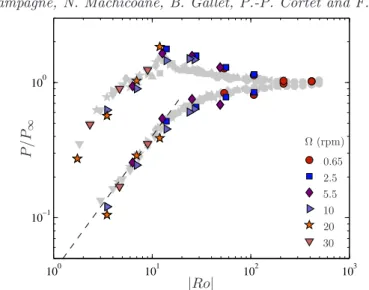
100 101 102 103 10−1 100 Ω (rpm) P /P ∞ |Ro| 0.65 2.5 5.5 10 20 30
Figure 6.Dissipated power P , estimated by the turbulent fluctuations u′
pof the poloidal flow measured through stereoscopic PIV, using the non-rotating estimate u′3
p/h, and normalized by its non-rotating value P∞. The good agreement between P/P∞and the input power K/K∞ measured from torque data (data shown as faint symbols reproduced from figure 2) demonstrates that the non-rotating estimate u′3
p/h correctly describes the energy dissipation rate, even in the rotating case.
On a qualitative level, these observations therefore support the partial two-dimensionalization scenario: most of the kinetic energy of the rapidly-rotating flow corresponds to 2D z-invariant motion, which is discarded at the outset of wave turbulence theories. A quantitative criterion is however needed to distinguish more clearly between the two scenarios. To wit, we evaluate the energy dissipation rate of the turbulent poloidal flow directly from the PIV measurements: assuming that the energy-containing scale is given by the impeller height h, the non-rotating estimate of this quantity is u′3
p/h, whereas the wave turbulence estimate is u ′4
p/Ωh2. We compute
the spatial integral of the non-rotating estimate u′3
p/h in the vicinity of the impeller,
inside the dashed region shown in the upper-right panel of figure 4. We denote as P the resulting quantity, and report its behavior with Ro in figure 6. It matches remarkably the behavior of K, both curves being normalized by their asymptotic non-rotating value, with K∞/P∞= 0.6±0.1. This good agreement confirms that energy dissipation is mostly
due to the 3D part of the flow, the laminar dissipation of the 2D flow being negligible. But more importantly, for the moderate Rossby numbers studied here, it demonstrates that energy dissipation can be estimated locally from the usual non-rotating scaling-law u′3
p/h, ruling out the modified energy dissipation u ′4
p/Ωh2predicted by weak turbulence
theory (such non-rotating scaling-law is also consistent with studies of grid-generated rotating turbulence (Hopfinger et al. 1982; Staplehurst et al. 2008; Moisy et al. 2011), which showed that the small-scale turbulent fluctuations start developing some rotation-induced anisotropy for Ro′
.0.2 only). The quantitative criterion illustrated in figure 6 allows to clearly discriminate between the two scenarios, and we conclude that drag reduction originates from a partial two-dimensionalization of the flow, with reduced 3D turbulent fluctuations.
Turbulent drag in a rotating frame 9
5. Concluding remarks
The two-dimensionalization scenario for drag reduction is supported so far by the vertical axis configuration (figure 1b,c), which is compatible with the Taylor-Proudman theorem. What if the axis of the impeller is horizontal (see figure 1d)? Such a configura-tion is incompatible with the Taylor-Proudman theorem: there is no vertically invariant flow solution compatible with the boundary conditions, even for a perfect fluid, because of the nonzero vertical velocity imposed by the impeller. This geometry therefore prohibits the partial two-dimensionalization scenario, while it still allows for the inertial-wave one. The vertical motion of the blades induces 3D turbulent velocity fluctuations of order Rω, regardless of Ro. The usual non-rotating estimate for the energy dissipation rate then gives R3ω3/h, from which we predict no dependence of K on Ro, whereas the
wave turbulence prediction gives R4ω4/h2Ω, with a strong decrease in drag coefficient
K ∼ Ro for decreasing Ro. Once again, the data in figure 2 clearly depart from the wave-turbulence prediction: for the moderate Rossby numbers considered here, there is no drop in drag coefficient in this horizontal-axis configuration.
To conclude, we observe strong drag reduction whenever two-dimensionalization is allowed, i.e., when the forcing geometry is compatible with the Taylor-Proudman the-orem: the drag coefficient is dramatically reduced for motion perpendicular to the global rotation axis, while it is very weakly affected for motion parallel to the global rotation axis. Importantly, for the moderate Rossby numbers considered here, the energy dissipation rate obeys the classical non-rotating scaling-law, and not the wave-turbulence one. The decrease in drag is a consequence of a decrease in 3D turbulence intensity, in line with the two-dimensionalization of the large-scale flow. It would be of great interest to achieve even faster global rotation, to determine how the flow approaches the asymptotic 2D state: is there a threshold Ro under which the flow becomes exactly 2D (up to boundary layers), as in the stress-free case considered by Gallet (2015), or is there a clear-cut scaling-law governing the decrease in 3D energy as a function of Ro?
Such experiments would also indicate how much further the drag can be reduced: for very fast global rotation, the decrease in bulk dissipation may be hidden by increasing Ekman friction in the boundary layers, which probably becomes the dominant cause of dissipation for large Ω. As a consequence, there would be an optimum rotation rate that leads to a minimum in drag.
We acknowledge S. Fauve for providing the fruitful seed idea, and A. Aubertin, L. Auffray, C. Borget and R. Pidoux for their experimental help. This work is supported by “Investissements d’Avenir” LabEx PALM (ANR-10-LABX-0039-PALM). F.M. acknowl-edges the Institut Universitaire de France.
REFERENCES
Alexakis, A.2015 Rotating Taylor-Green flow. J. Fluid Mech. 769, 46.
Baqui, Y. B. & Davidson, P. A. 2015 A phenomenological theory of rotating turbulence. Phys. Fluids 27, 025107.
Cambon C. & Jacquin, L.1989 Spectral approach to non-isotropic turbulence subjected to rotation. J. Fluid Mech. 202, 295.
Cambon, C., Rubinstein, R. & Godeferd, F. S.2004 Advances in wave turbulence: rapidly rotating flows. New J. Phys. 6, 73.
Campagne, A., Gallet, B., Moisy, F. & Cortet, P.-P. 2014 Direct and inverse energy cascades in a forced rotating turbulence experiment. Phys. Fluids 26, 125112.
Campagne, A., Gallet, B., Moisy, F., & Cortet, P.-P.2015 Disentangling inertial waves from eddy turbulence in a forced rotating turbulence experiment. Phys. Rev. E 91, 043016. Clark di Leoni, P., Cobelli, P. J., Mininni, P. D., Dmitruk, P. & Matthaeus, W. H.
2014 Quantification of the strength of inertial waves in a rotating turbulent flow. Phys. Fluids. 26, 035106.
Davidson, P. A. 2013 Turbulence in Rotating, Stratified and Electrically Conducting Fluids. Cambridge University Press.
Dubrulle, B., Dauchot, O., Daviaud, F., Longaretti, P.-Y., Richard, D. & Zahn, J.-P. 2005 Stability and turbulent transport in Taylor-Couette flow from analysis of experimental data. Phys. Fluids. 17, 095103.
Frisch, U.1995 Turbulence - The Legacy of A. N. Kolmogorov. Cambridge University Press. Gallet, B.2015 Exact two-dimensionalization of rapidly rotating large-Reynolds-number flows
J. Fluid Mech. 783, 412-447.
Galtier, S.2003 Weak inertial-wave turbulence theory. Phys. Rev. E 68, 015301.
Godeferd, F. S. & Moisy, F.2015 Structure and dynamics of rotating turbulence: a review of recent experimental and numerical results. Appl. Mech. Rev. 67, 030802.
Greenspan, H.1968 The theory of rotating fluids. Cambridge University Press.
Hide, R. & Titman, C. W.1967 Detached shear layers in a rotating fluid. J. Fluid Mech. 29, 1.
Hopfinger, E.J., Browand, F.K. & Gagne, Y. 1982 Turbulence and waves in a rotating tank. J. Fluid Mech. 125, 505-534.
Iroshnikov, P. S.1964 Turbulence of a Conducting Fluid in a Strong Magnetic Field. Soviet Astronomy 7, 4.
Kloorsterziel, R. C. & Van Heijst, G. J. F. 1991 An experimental study of unstable barotropic vortices in a rotating fluid. J. Fluid Mech. 223, 1.
Kraichnan, R. H.1965 Inertial-range spectrum of hydromagnetic turbulence. Phys. Fluids 8, 1385.
Moisy, F., Morize, C., Rabaud, M. & Sommeria, J. 2011 Decay laws, anisotropy and cyclone-anticyclone asymmetry in decaying rotating turbulence. J. Fluid Mech. 666, 5-35. Mutabazi, I., Normand, C. & Wesfreid, J. E. 1992 Gap size effects on centrifugally and
rotationally driven instabilities. Phys. Fluids 4, 1199. Nazarenko, S.2011 Wave Turbulence. Springer-Verlag.
Ostilla-M´onico, R., Huisman, S. G., Jannink, T. J. G., Van Gils, D. P. M., Verzicco, R., Grossmann, S., Sun, C. & Lohse, D. 2014 Optimal Taylor-Couette flow: radius ratio dependence. J. Fluid Mech. 747, 1.
Paoletti, M. S. & Lathrop, D. P.2011 Angular Momentum Transport in Turbulent Flow between Independently Rotating Cylinders. Phys. Rev. Lett. 106, 024501.
Smith, L. M., Chasnov, J. R. & Waleffe F. 1996 Inertial transfers in the helical decomposition. Phys. Rev. Lett. 77, 2467.
Staplehurst, P.J., Davidson, P.A. & Dalziel, S.B. 2008 Structure formation in homogeneous freely decaying rotating turbulence. J. Fluid Mech. 598, 81-105.
Van Gils, D. P. M., Huisman, S. G., Bruggert, G.-W., Sun, C., & Lohse, D.2011 Torque scaling in turbulent Taylor-Couette flow with co- and counterrotating cylinders. Phys. Rev. Lett. 106, 024502.
Yarom E. & Sharon E.2014 Experimental observation of steady inertial wave turbulence in deep rotating flows. Nature Phys. 10, 510-514.