The MIT Faculty has made this article openly available. Please share
how this access benefits you. Your story matters.
Citation Guo, Syuan-Ming, Jun He, Nilah Monnier, Guangyu Sun, Thorsten Wohland, and Mark Bathe. “Bayesian Approach to the Analysis of Fluorescence Correlation Spectroscopy Data II: Application to Simulated and In Vitro Data.” Analytical Chemistry 84, no. 9 (May 2012): 3880–3888.
As Published http://dx.doi.org/10.1021/ac2034375
Publisher American Chemical Society (ACS)
Version Author's final manuscript
Citable link http://hdl.handle.net/1721.1/92290
Terms of Use Creative Commons Attribution-Noncommercial-Share Alike
A Bayesian approach to the analysis of fluorescence correlation spectroscopy data II:
Application to simulated and in vitro data
Journal: Analytical Chemistry Manuscript ID: ac-2011-034375.R1 Manuscript Type: Article
Date Submitted by the
Author: 12-Mar-2012
Complete List of Authors: Guo, Syuan-Ming; Massachusetts Institute of Technology, Chemistry He, Jun; Massachusetts Institute of Technology, Biological
Engineering
Monnier, Nilah; Massachusetts Institute of Technology, Biological Engineering
Guangyu, Sun; National University of Singapore, Chemistry and Centre for Bioimaging Sciences
Wohland, Thorsten; National University of Singapore, Chemistry and Centre for Bioimaging Sciences
Bathe, Mark; MIT, Biological Engineering
177x203mm (300 x 300 DPI) 3 4 5 6 7 8 9 10 11 12 13 14 15 16 17 18 19 20 21 22 23 24 25 26 27 28 29 30 31 32 33 34 35 36 37 38 39 40 41 42 43 44 45 46 47 48 49 50 51 52 53 54 55 56 57 58
106x190mm (300 x 300 DPI) 3 4 5 6 7 8 9 10 11 12 13 14 15 16 17 18 19 20 21 22 23 24 25 26 27 28 29 30 31 32 33 34 35 36 37 38 39 40 41 42 43 44 45 46 47 48 49 50 51 52 53 54 55 56 57
456x316mm (171 x 171 DPI) 3 4 5 6 7 8 9 10 11 12 13 14 15 16 17 18 19 20 21 22 23 24 25 26 27 28 29 30 31 32 33 34 35 36 37 38 39 40 41 42 43 44 45 46 47 48 49 50 51 52 53 54 55 56 57 58
469x229mm (300 x 300 DPI) 3 4 5 6 7 8 9 10 11 12 13 14 15 16 17 18 19 20 21 22 23 24 25 26 27 28 29 30 31 32 33 34 35 36 37 38 39 40 41 42 43 44 45 46 47 48 49 50 51 52 53 54 55 56 57
143x227mm (300 x 300 DPI) 3 4 5 6 7 8 9 10 11 12 13 14 15 16 17 18 19 20 21 22 23 24 25 26 27 28 29 30 31 32 33 34 35 36 37 38 39 40 41 42 43 44 45 46 47 48 49 50 51 52 53 54 55 56 57 58
A Bayesian approach to the analysis of fluorescence correlation spectroscopy data II: Application to simulated and in vitro data
Syuan-Ming Guo1, Jun He1, Nilah Monnier1, Guangyu Sun2, Thorsten Wohland2, Mark Bathe1* 1Laboratory for Computational Biology & Biophysics, Department of Biological Engineering,
Massachusetts Institute of Technology, Cambridge, MA 02139, USA
2Department of Chemistry and Centre for Bioimaging Sciences, National University of Singapore, 117543 Singapore
KEYWORDS fluorescence correlation spectroscopy, multiple hypothesis testing, Bayesian
inference, statistical accuracy, diffusion
*Corresponding Author: Mark Bathe 77 Massachusetts Avenue Building 16, Room 255 Cambridge, MA 02139, USA Tel. (617) 324-5685 Fax (617) 324-7554 [email protected] 3 4 5 6 7 8 9 10 11 12 13 14 15 16 17 18 19 20 21 22 23 24 25 26 27 28 29 30 31 32 33 34 35 36 37 38 39 40 41 42 43 44 45 46 47 48 49 50 51 52 53 54 55 56 57
ABSTRACT
Fluorescence Correlation Spectroscopy (FCS) is a powerful approach to characterizing the binding and transport dynamics of macromolecules. The unbiased interpretation of FCS data relies on the evaluation of multiple competing hypotheses to describe an underlying physical process under study, which is typically unknown a priori. Bayesian inference provides a convenient framework for this evaluation based on the temporal autocorrelation function (TACF), as previously shown theoretically using model TACF curves1. Here, we apply this procedure to simulated and experimentally measured photon-count traces analyzed using a multi-tau correlator, which results in complex noise properties in TACF curves that cannot be modeled easily. As a critical component of our technique, we develop two means of estimating the noise in TACF curves based either on multiple independent TACF curves themselves or a single raw underlying intensity trace, including a general procedure to ensure that independent, uncorrelated samples are used in the latter approach. Using these noise definitions, we demonstrate that the Bayesian approach selects the simplest hypothesis that describes the FCS data based on sampling and signal limitations, naturally avoiding over-fitting. Further, we show that model probabilities computed using the Bayesian approach provide a reliability test for the downstream interpretation of model parameter values estimated from FCS data. Our procedure is generally applicable to FCS and image correlation spectroscopy, and therefore provides an important advance in the application of these methods to the quantitative biophysical investigation of complex analytical and biological systems.
3 4 5 6 7 8 9 10 11 12 13 14 15 16 17 18 19 20 21 22 23 24 25 26 27 28 29 30 31 32 33 34 35 36 37 38 39 40 41 42 43 44 45 46 47 48 49 50 51 52 53 54 55 56 57 58
INTRODUCTION
Fluorescence Correlation Spectroscopy (FCS) is an established technique to measure molecular dynamics ranging from binding to transport in living and non-living samples2-6. As with all measurements, interpretation of FCS data relies on an inference process in which multiple competing hypotheses are tested for the ability to describe the physical process under study, which is generally assumed to be unknown a priori, followed by interpretation of parameter values of the inferred model. Controlled molecular or other perturbations to the system then provide insight into the mechanistic origin of the inferred model, as well as its parameter values.
Broad application of FCS to biological and other complex systems has in part been hindered by sample heterogeneity7-9 and measurement limitations that include low signal-to-noise ratios10, non-stationarity of the physical process under study, and photobleaching11, which render objective interpretation of FCS data challenging12-14. As a first step towards overcoming these obstacles in order to apply FCS broadly to complex chemical systems, we recently developed a multiple hypothesis-testing framework that is based on Bayesian inference that enables the automatic, objective evaluation of multiple competing models in the interpretation of FCS data from Temporal Autocorrelation Functions (TACFs)1. In that work, we simulated analytical TACFs from various transport processes with controlled noise features in order to test systematically the ability of the proposed procedure to detect the underlying physical process in the presence of various types of noise and data limitations that are characteristic of FCS applications. Precise and independent control of these distinct noise and sampling properties of the TACF, in addition to the physical transport process, were essential to enable the systematic evaluation of the proposed theoretical procedure in a controlled setting without the complicating features of real measurements noted above.
In conventional FCS, fluorescence fluctuations are measured in femtoliter volumes at a fixed spatial position (or series of positions) using a sensitive photon counting device such as a Photomultiplier Tube (PMT) or Avalanche Photodiode (APD)15-17. TACFs are subsequently computed from measured photon counts using a hardware correlator. These intensity-derived TACFs have characteristic noise features that cannot be controlled independently because they depend nonlinearly both on various features of the measurement system as well as on the manner in which the correlation function itself is computed. For example, multi-tau correlators result in 3 4 5 6 7 8 9 10 11 12 13 14 15 16 17 18 19 20 21 22 23 24 25 26 27 28 29 30 31 32 33 34 35 36 37 38 39 40 41 42 43 44 45 46 47 48 49 50 51 52 53 54 55 56 57
correlated, inhomogeneous noise that decays with increasing lag-time18-20, whereas uniform sliding window averaging used to compute the TACF in image correlation spectroscopy results in correlated but largely homogeneous noise21. Existing theoretical models for noise levels in TACFs are derived assuming particular forms of the correlation function such as an exponential or single hyperbolic function and therefore cannot be applied to FCS data from physical processes containing more complex correlations18, 20, 22, 23. Calculating standard deviations of multiple TACFs measured from the same physical process provides one model-free procedure to estimating the noise in TACFs20, 24. However, the large number of repeated measurements required for a reliable estimate of standard deviation is time-consuming and not always feasible for a non-stationary system. Importantly, Schätzel et al.19 previously showed that ignoring noise correlations in the analysis of TACFs may result in over-fitting and therefore improper interpretation of FCS data. Notwithstanding, noise correlations are still typically ignored in the analysis and interpretation of TACFs due to the lack of suitable procedures for their estimation.
To apply the theoretical Bayesian framework1 to FCS data from fluorescence intensity traces, we investigate here its ability to infer the known physical process of multi-component diffusion based on TACFs computed from simulated and experimental fluorescence intensity traces under various measurement and sampling conditions. As a critical component of the application of our procedure, we present two approaches to estimating the noise magnitude and its correlation from either multiple independent TACF curves or a single photon-count trace. In the latter, we introduce an analysis procedure that ensures that the noise covariance matrix is properly estimated from underlying intensity traces, eliminating potential bias introduced by over-fitting TACF data. Following Wohland et al.20, fluorescence intensity traces are simulated from single-particle diffusion and fluorescence emission and collection from a confocal volume to control and vary systematically fluorophore emission and light collection properties, which is impossible in real experiments. Importantly, TACFs calculated from simulated and real intensity traces have noise properties that cannot be modeled and therefore investigated using our previous approach that applied Bayesian inference to model TACFs with superposed simulated noise1. Subsequently, we apply the procedure to examine the effect of triplet fraction of excited fluorescence molecules and molecular diffusion from experimental samples of aqueous Atto565 and Atto565-labeled Streptavidin solutions. Subsequent developments will focus on the application of the proposed Bayesian approach to biological samples in which additional 3 4 5 6 7 8 9 10 11 12 13 14 15 16 17 18 19 20 21 22 23 24 25 26 27 28 29 30 31 32 33 34 35 36 37 38 39 40 41 42 43 44 45 46 47 48 49 50 51 52 53 54 55 56 57 58
important complexities beyond those encountered here are present, including non-stationarity of the underlying physical process, sample heterogeneity, and photobleaching.
THEORY FCS models
The TACF of fluctuations in the measured fluorescence intensity is calculated using,
(1)
where is the fluctuation of the measured fluorescence intensity and brackets denote ensemble average, which is equal to the time-average if the system is ergodic25.
For a system of non-interacting fluorescent species undergoing normal diffusion and a 3D Gaussian ellipsoid focal volume with transverse width and height 0, the TACF has the closed-form solution2, 17, 26, 27,
1 1 (2)
where 2 / ∑ 2 and 02/4 are the correlation amplitude and the
diffusion time of component , respectively. / is the aspect ratio of the focal volume or the molecule detection function (MDF)28, and is the brightness of component and is given by , where is the absorption cross-section of the fluorophore, is the quantum yield of fluorophores, is the overall transmittance of the optics that accounts for total photon loss due to light transmission and collection of optical components, is the quantum efficiency of the detection device.
In the case of high illumination intensity, the high fraction of molecules being excited to the non-fluorescent triplet state results in additional fluctuations in intensity on a short time scale, which can be described by29,
3 4 5 6 7 8 9 10 11 12 13 14 15 16 17 18 19 20 21 22 23 24 25 26 27 28 29 30 31 32 33 34 35 36 37 38 39 40 41 42 43 44 45 46 47 48 49 50 51 52 53 54 55 56 57
1
1 exp , (3)
where is the mean fraction of molecules in the triplet state, and is the triplet blinking time. increases with increasing illumination intensity and can be approximated by
when 1 or .
Bayesian model selection
The detailed theory for the Bayesian inference procedure based on TACF curves is described in previous work1. In that work, various distributions of noise were assumed in order to test the approach generally, whereas here we compute the noise directly from the multi-tau correlator. This results in non-uniform and correlated noise due in part to the sampling time that increases with increasing lag-time, . The data probability given by the parameters of the model is described by a general multivariate general multivariate normal distribution,
, (4)
where , , … , is the data vector of the measured TACF, is the
analytical TACF FCS model with the vector of sampled lag time , , … , and the
parameter vector , and is the covariance matrix of the errors in the measured TACF values. Modeling the noise in the TACF with the normal distribution is justified by the central limit theorem because each value in the TACF is the average of a large number of the underlying intensity products (Eq. 1 and Supporting Information, S1). The nonlinear regression process that seeks the maximum-likelihood estimate to maximize Eq. 4 is called generalized least squares (GLS), in contrast to weighted least squares (WLS), in which independent errors are assumed30. The estimation of for the TACF is described in later sections.
The probability of model given the observed data is given by Bayes’ theorem, β ( , ) f x β T 1 /2 1 1 ( | ) exp [ ( , )] [ ( , )] 2 (2 )n det( ) P f f y β y x β C y x β C ( , ) f x β β C MLE β C k P M y( k ) 3 4 5 6 7 8 9 10 11 12 13 14 15 16 17 18 19 20 21 22 23 24 25 26 27 28 29 30 31 32 33 34 35 36 37 38 39 40 41 42 43 44 45 46 47 48 49 50 51 52 53 54 55 56 57 58
, (5)
where the proportionality holds if the prior probabilities of all the models are equal for all . Because the normalized model probability is typically reported, in practice we only need to know the marginal likelihood of the data, .
in Eq. 5 is obtained by an integral over the parameter space , which can be evaluated analytically using the Laplace approximation that is asymptotically exact,
(6)
where is the maximum of the posterior distribution of parameters , or the Bayesian point estimate, and is the covariance matrix of estimated at . When a uniform prior in the parameter space is chosen, and are equivalent to and . Use of the Laplace approximation is justified when the posterior distribution of the parameters approaches a Gaussian, as was shown in our previous work to be the case for typical TACF curves1. Once is computed, model probabilities may be calculated using Eq. 5. Calculation of the probabilities of a set of competing models for describing FCS data thereby enables their direct comparison and evaluation in the presence of measurement noise, data limitations, as well as sample heterogeneity, though we explore only the first two features of FCS data in this work.
Estimation of noise and noise correlations from multiple TACFs
Proper estimation of the noise and the noise correlation in the TACF is essential for the calculation of model probabilities using Bayesian inference, as well as for accurate parameter estimation20. We present two independent approaches to estimating the covariance matrix in
( ) ( ) ( ) ( ) ( ) k k k k P M P M P M P M P y y y y k ( k) P y M ( k) P y M ( k) ( , k) ( k) P M
P M P M d β y y β β β /2 1/2 ˆ ˆ ( ) (2 )p | | ( ) ( | )k Bayes Bayes k Bayes k
P | My P y | β M P β M ˆ Bayes β P(β y,Mk) Bayes Σ β βˆBayes ˆ Bayes
β Bayes βˆMLE MLE
( k) P y M C 3 4 5 6 7 8 9 10 11 12 13 14 15 16 17 18 19 20 21 22 23 24 25 26 27 28 29 30 31 32 33 34 35 36 37 38 39 40 41 42 43 44 45 46 47 48 49 50 51 52 53 54 55 56 57
Figure 1 Flowchart of Bayesian model selection procedures for FCS data of multiple TACF
curves or a single intensity trace. See text for details. 3 4 5 6 7 8 9 10 11 12 13 14 15 16 17 18 19 20 21 22 23 24 25 26 27 28 29 30 31 32 33 34 35 36 37 38 39 40 41 42 43 44 45 46 47 48 49 50 51 52 53 54 55 56 57 58
Eq. 4 for distinct types of FCS data (Fig. 1). First, when multiple independent TACF curves measured from the same physical process are available, may be estimated by calculating the sample covariance matrix using all TACF curves. The matrix elements in the sample covariance matrix are given by,
(7)
where denotes the total number of TACF curves analyzed and denotes an individual curve j. The covariance of the mean curve from the average of individual curves is then given by 1⁄ . However, this sample-based estimate of the covariance matrix is only well-conditioned when the number of observations (i.e., the number of available independent TACF curves) is much larger than the dimension of , which is generally not true for high dimensional data such as TACF curves (typically 128 points). Therefore, we use the regularized shrinkage estimator for covariance matrices to ensure that the estimated matrix is well-conditioned and has lower mean squared error (MSE) than the sample covariance matrix31, 32. The shrinkage estimator for the covariance is typically the linear combination of the sample covariance matrix and a low dimensional shrinkage target,
(8)
where is the shrinkage target, which is usually diagonal, and is the optimal shrinkage weight associated with the specific shrinkage target. The shrinkage weight depends on the uncertainty in , which is determined by the number of samples from which is calculated. decreases monotonically as the number of available samples increases so that approaches asymptotically. While we found that different shrinkage targets all reduce the MSE and yield well-conditioned estimates for the covariance structure of the noise in the TACF, we choose the “two-way” target33 here because it preserves the correlation structure and yields smaller uncertainty in model probabilities at the same time (Supporting Information, S2).
C S Skl S Skl 1 J1 G ( j)( k)G(k)
G( j )( l)G(l)
j1 J
J G( )j ( ) ( )l G J C * (1 ) S T S T
S S
* S S 3 4 5 6 7 8 9 10 11 12 13 14 15 16 17 18 19 20 21 22 23 24 25 26 27 28 29 30 31 32 33 34 35 36 37 38 39 40 41 42 43 44 45 46 47 48 49 50 51 52 53 54 55 56 57Estimation of noise and noise correlations from a single photon-count trace
Estimating the noise from multiple TACF curves is only justified when all of the curves come from repeated measurements of the same physical process and the variation across curves is purely from intrinsic statistical error in the correlation function estimator due to the finite sample size. However, in applications of FCS to in vivo biological data it may be preferable to evaluate model probabilities directly from the same, single sample. In this case, an alternative approach is to estimate the noise in a single TACF by calculating the noise from the underlying photon-count products20, assuming that the raw photon-count trace or photon arrival time information is available. For the multi-tau correlator, the TACF for a photon-count trace with an acquisition time Taq is calculated from
(9) with (10)
where is the sampling time (or channel width) used to calculate , is the photon count at , , , and M Taq i k is the number of possible
products . According to Eq. 9, because G
is the mean of the underlying photon-count products, the covariance of and may be calculated from these underlying samples .Note that calculating the variance or covariance in the photon-count products between time lags requires either independent samples of these products at each or knowledge of the correlations between the samples of these products at each , otherwise the noise level will be underestimated. For FCS data, the photon-count products at any are not
1 0 1 ( ) M m m k m k i k n n M G G k n n
1 1 M j m j m n n M
i G
k nm i m nmnmn0 nm k nm k nk m m k n n
k G G
l
,
1 M m m k m m l m n n n n k k
1 M m m k m n n k 3 4 5 6 7 8 9 10 11 12 13 14 15 16 17 18 19 20 21 22 23 24 25 26 27 28 29 30 31 32 33 34 35 36 37 38 39 40 41 42 43 44 45 46 47 48 49 50 51 52 53 54 55 56 57 58independent and their correlations are given by a fourth-order correlation function23, 24. Here we introduce a procedure to circumvent this problem by performing a block-transformation on the photon-count products to obtain independent samples34. This approach is used extensively in the molecular simulation community to obtain independent estimates from highly correlated molecular trajectories35. The covariance matrix of the mean can then be calculated directly from these transformed, independent samples without the evaluation of the higher order correlation function.
The blocking method seeks the minimal averaging time (or block-time) beyond which the transformed samples (or the block-averages) of the photon-count products are no longer
correlated. Defining Eq. 9 becomes,
. (11)
The block-transformed sample pm
kwith the block-time is given by the block-average of all
within , namely,
1 1
1 2
1 m m m m p k p k p k p k (12)where is the number of samples in the block. The covariance between pm
k at different decrease as increases because correlations between the underlying photon count decay over time. Note that Eq. 11 still holds for the transformed samples pm
k , so the covariance of and can be calculated from pm
k as well. When is beyond the minimal block-time needed to obtain independent blocked samples, the matrix elements in the sample covariance matrix of can be calculated directly from these independent transformed samples:
0 m m k m k n n p k n n
1 1 ( i) M m m G k p k M
b t
m p k tb b i t m tb
k G G
l tb kl S S G( ) 3 4 5 6 7 8 9 10 11 12 13 14 15 16 17 18 19 20 21 22 23 24 25 26 27 28 29 30 31 32 33 34 35 36 37 38 39 40 41 42 43 44 45 46 47 48 49 50 51 52 53 54 55 56 57(13)
where is the number of transformed samples. The minimal block-time depends on the correlation time of the measured physical process and the functional form of its decay. In practice, the minimal block-time can be determined by plotting at as a function of the block-time , and finding the minimal time after which becomes invariant to 34, 35.
RESULTS AND DISCUSSION
Effects of acquisition parameters and physical processes on model probabilities when multiple TACF measurements are available
To evaluate the performance of the proposed Bayesian analysis procedures we first apply Approach 1 (Fig. 1) to TACF curves computed from simulated fluorescence intensity traces of two species with the same brightness undergoing normal diffusion and test their ability to detect the two species for varying conditions of acquisition and physical processes typically encountered experimentally (Supporting Information, S3 and S4). The noise correlation calculated from multiple TACF curves has a structure consistent with the expected noise correlation structure for a TACF curve calculated from a multi-tau correlator (Fig. 2B)19, 24. At small the noise is dominated by uncorrelated photon counting noise due to the short sampling time ( ) there. As increases with increasing , the photon count increase and the noise becomes dominated by intensity fluctuations from particle motions, which are highly correlated on the time-scale of diffusion in the focal volume. When is much larger than the correlation time , the noise in this regime becomes uncorrelated again because intensity fluctuations are uncorrelated on this time-scale.
To investigate systematically the effect of variable experimental noise, which can result from low count rate of the particles or insufficient acquisition time, on the ability of the Bayesian approach to identify the number of components present, we varied the optical transmittance or the acquisition time of the photon-count trace and calculated model probabilities from the resulting TACF curves. Again, the noise levels and correlations in TACFs are estimated using multiple curves as in Approach 1 (Fig. 3A and B). As observed in our previous work1, the
1
1 1 M kl m m m S p k p k p l p l M M
M kk S k b t Skk tb i i i i i D T 3 4 5 6 7 8 9 10 11 12 13 14 15 16 17 18 19 20 21 22 23 24 25 26 27 28 29 30 31 32 33 34 35 36 37 38 39 40 41 42 43 44 45 46 47 48 49 50 51 52 53 54 55 56 57 58Figure 2 (A) Generalized least-squares fits of the one- and two-component models to the mean,
G , of eight individual TACFs, G( )j
, where each G( )j
is computed using the multi-tau algorithm from a simulated photon-count trace of two distinct, point-like fluorescent species with the same brightness undergoing normal diffusion. 34 particles with D1 63.1 μm2/sec and 35 particles with D2 121.8 μm2/sec are simulated in a sphere of 3 μm radius, corresponding to a mean concentration of 1 nM, with P100 W , 514.5 nm, 2.2 10 m 12 2abs , ,
0.01
, pinhole diameter 50 μm, and acquisition time 3.3 sec, corresponding to count rates of ~35 kHz for each species. Errors bars denote noise in the mean TACF estimated using Approach 1 (see text for details). Normalized residuals from the two fits are shown in the lower panel. (B) Shrinkage estimate of the noise correlation matrix in G
estimated from 64 individual TACF curves calculated from simulated photon-count traces with the same simulation parameters as in (A) except D1 270 μm2/sec and D2 27 μm
2/sec. The simulation parameters in (B) are used for all simulations in future figures unless otherwise noted.
0.98 f q 3 4 5 6 7 8 9 10 11 12 13 14 15 16 17 18 19 20 21 22 23 24 25 26 27 28 29 30 31 32 33 34 35 36 37 38 39 40 41 42 43 44 45 46 47 48 49 50 51 52 53 54 55 56 57
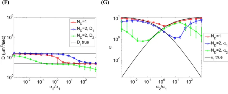
Figure 3 Bayesian analysis of simulated two-component diffusion using Approach 1. Eight
mean TACF curves are fit to obtain each data point, where each mean TACF is the average of eight individual TACF curves generated using the same simulation parameters as in Fig. 2B. The noise correlation matrix is estimated using 64 individual TACFs and regularized using the shrinkage estimator as described in the main text. (A-E) Inferred model probabilities as a function of (A) κ, (B) acquisition time, (C) minimum sampling time, (D)
2/ 1, and (E)2/ 1
D D. (F) Diffusion coefficients obtained from the one- and two-component model fits in (E). Black lines represent the prescribed values of D1 and D2 for the two-component model. (G) N values obtained from the one- and two-component model fits in (E). The black lines represent the prescribed N values for the two-component model. In all cases, medians and upper and lower quartiles are shown for the eight mean curves analyzed for each data point. In (A) and (B), the lower panels show the relative noise level
0 G0 in the TACF curves, which is calculated by averaging over the first 16 values in
|G
|. The count rate per particle corresponding to the range of κ scanned in (A) is 0.35-350 kHz. A background with count rate of 5 kHz was added to the signal before detection in (A) to avoid zero correlation at low .
0 G0 is not monotonically decreasing in (A) because the signal at low is almost from the uncorrelated background and results in noisy TACFs with in (E) is varied by changing whileholding fixed at 63.1 μm2/sec.
2/ 1 D D D2 1 D 3 4 5 6 7 8 9 10 11 12 13 14 15 16 17 18 19 20 21 22 23 24 25 26 27 28 29 30 31 32 33 34 35 36 37 38 39 40 41 42 43 44 45 46 47 48 49 50 51 52 53 54 55 56 57 58Bayesian procedure resolves the two-component model at low noise levels, but prefers the one-component model when the noise level increases because the additional complexity of the two-component model is not justified there given the uncertainty in the TACF data. Importantly, the three-component model is never preferred, demonstrating that the Bayesian approach does not over-fit the data. While the maximum relative noise level ( ) that can be tolerated for the Bayesian approach to resolve the two-component model is found here to be ~10%, this maximum relative noise level depends on the separation of the diffusion times and the relative amplitudes of the two components.
The minimum sampling time is also expected to eliminate the ability of the Bayesian approach to resolve the two species. When the minimum sampling time exceeds the diffusion time of the fast diffusing component (55 μs), the fast component is no longer apparent in the TACF curve and the Bayesian approach correspondingly prefers the one-component model (Fig. 3C). While the sampling time is not generally a concern for single-point FCS measurements using APDs or PMTs, limitations in minimum sampling time are of major concern in image-based FCS methods where sampling time is on the scale of milliseconds or longer21, 36-39.
Next we examined the effect of varying the underlying physical process by varying the relative brightness of the two species, which alters their relative amplitudes (Fig. 3D). Experimentally, may vary due to differences either in the brightness or the concentration of the particles examined. When the amplitudes of the two components are similar ( ~ 1), the Bayesian approach is able to resolve the two species (Fig. 3D). In contrast, when the relative amplitude of the two components becomes considerably different from unity, the contribution to the TACF from one of the species is too small to be detected above the noise so that the Bayesian procedure prefers the simpler, one-component model (Fig. 3D). Similar to the effect of varying , the ability of the Bayesian approach to resolve the two species depends on the ratio of their diffusion coefficients (Fig. 3E). When and are approximately equal, the simpler one-component model is preferred because the two components cannot be sufficiently resolved due to their similar diffusion time-scales, as observed previously1. Outside of this regime, the two-component model is preferred because the diffusion time-scales of the two components are well separated and can be distinguished at the given noise level. Again, the over-parameterized three-component model is never preferred. Note that the transition in model
0 G0 i B
2/ 1
2/ 1
2/
1
2 / 1 D D D2 D1 3 4 5 6 7 8 9 10 11 12 13 14 15 16 17 18 19 20 21 22 23 24 25 26 27 28 29 30 31 32 33 34 35 36 37 38 39 40 41 42 43 44 45 46 47 48 49 50 51 52 53 54 55 56 57probabilities at is sharper than the transition at . This is because the value of is smaller in the latter case, and slower diffusion of particles increases the variability in observed TACF curves given a fixed observation time, increasing noise and reducing the ability to resolve complex models.
The parameter estimates from the two-component model are reliable when the probability of this model is high, and become less reliable when the model probability is low, with greater uncertainty in the latter case (Figure 3F, 3G, and S3). The estimated values of the diffusion coefficients are better predicted than the mean particle numbers when the two-component model probability is low because the system becomes effectively one-component when ⁄ 1. In this regime, and in the model need to be close to the overall effective diffusion coefficient, whereas the amplitudes and need only to satisfy the constraint , where is the overall amplitude. As a general rule, these results suggest that parameter estimates from a complex model should only be interpreted when this model is preferred decisively by the Bayesian inference procedure.
In contrast to accounting for noise correlations in the Bayesian procedure, we find that ignoring noise correlations as performed in conventional analysis of FCS data results in over-fitting due to the underestimation of the effective level of noise in the TACF (Fig. S4). The increase in mean model probabilities of complex models as well as uncertainties of model probabilities indicate noise correlations are over-fit by the extra component in more complex models when these correlations are not accounted for in the fitting process, whereas parameter estimates are more robust to ignoring noise correlations in TACFs (Fig. S5). Thus, for proper interpretation of FCS data, noise correlations should be considered for hypothesis testing of competing FCS models.
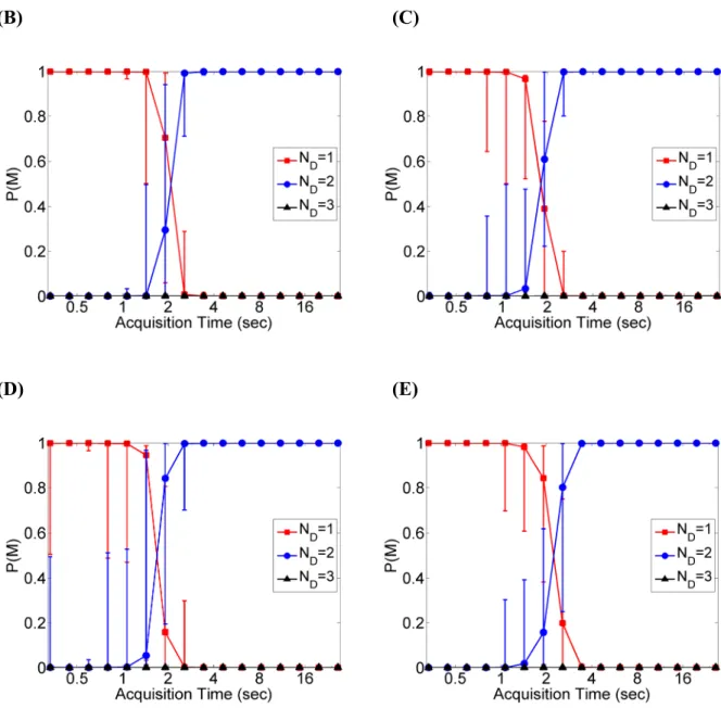
Application of the Bayesian approach to single intensity traces
When multiple TACF measurements are not available for a system of interest, the noise in a single TACF may be estimated directly from underlying photon-count products using the block-transformation procedure in Approach 2 (Fig. 1). The block-transformation results in increasing noise with increasing block-size , indicating the presence of correlation in samples
2/ 1 1 D D D D2/ 1 1 1 D 1 D D2 1 2 1 2 t t b t 3 4 5 6 7 8 9 10 11 12 13 14 15 16 17 18 19 20 21 22 23 24 25 26 27 28 29 30 31 32 33 34 35 36 37 38 39 40 41 42 43 44 45 46 47 48 49 50 51 52 53 54 55 56 57 58
Figure 4 (A) Estimated noise level in the value of at
= 10-5 sec as a function of block-time for two independent realizations (red and blue) of a simulated photon-count trace with simulation parameters = 0.01, D1270 μm2/sec, D2 27 μm2/sec, acquisition time of 26.4 sec, and background = 5 kHz. For both curves, the fixed point is reached at a block-time of approximately 20 msec. Error bars are standard deviations in the noise estimate assuming independent samples. (B) Estimated noise level in the TACF in (A) with and without the
blocking method. Block-time is 26.4 msec. (C) and (D) Bayesian analysis of simulated
two-component diffusion using Approach 2. Simulation parameters are identical to those in Fig. 3D and E except that each curve has an acquisition time of 26.4 sec so that the overall acquisition times in Fig. 3 and Fig. 4 are the same. (E) Diffusion coefficients obtained from the one- and
two-component model fits in (C). (F) N values obtained from the one- and two-component
model fits in (C). Medians and upper and lower quartiles are shown in (C-F) from the results of fitting eight individual TACF curves.
k G b t 3 4 5 6 7 8 9 10 11 12 13 14 15 16 17 18 19 20 21 22 23 24 25 26 27 28 29 30 31 32 33 34 35 36 37 38 39 40 41 42 43 44 45 46 47 48 49 50 51 52 53 54 55 56 57used to estimate the noise level (Fig. 4A). When , the rate of increase is small because fluctuations on this time-scale result primarily from uncorrelated photon counting noise. However, as the block-time increases to the scale ~ , the rate of increase is high because particle motion, which results in correlated intensity changes, is now the major source of the fluctuations. The estimated noise increases and approaches the true noise level because the covariance in the samples decreases with increasing . Finally, when (beyond the correlation time-scale of the particle motions), the transformed photon-count products become nearly independent and further increases in no longer change the estimated noise. Note that the statistical error in the noise estimate also grows with increasing block-size due to fewer samples at larger , therefore the choice of the optimal block-time is a trade-off between the bias and the variance in the noise estimate.
In practice, the optimal block-time (fixed point) can be determined by seeking the first point at which the noise estimate is invariant (within statistical error) to increasing . However, when the acquisition time is not considerably longer than the correlation time of the physical process, which in this case is the diffusion time-scale of the slower species, determining the fixed point might be hindered by the large error in the noise estimate due to the insufficient number of transformed samples. The noise level along the TACF estimated before and after the block-transformation using 26.4 ms exhibits a large increase due to the lack of correlations accounted in the samples by the former (Fig. 4B). Importantly, this apparent reduced error in the absence of the blocking procedure may clearly lead to over-fitting complex models to experimental FCS data.
To evaluate the performance of the Bayesian procedure with noise estimated from a single photon-count trace using the block-transformation, we apply Approach 2 to TACFs calculated from simulated intensity traces with varying simulation parameters as was performed in Fig. 3. Approaches 1 and 2 exhibit similar behaviors in terms of model probabilities and parameter estimates when data with equal simulation times are analyzed (Fig. 4C, D and S6). These results demonstrate that proper estimation of the noise and its correlations in the TACF may be obtained using the block-transformation when multiple independent measurements from a sample are not available. b t b t b t b t T 3 4 5 6 7 8 9 10 11 12 13 14 15 16 17 18 19 20 21 22 23 24 25 26 27 28 29 30 31 32 33 34 35 36 37 38 39 40 41 42 43 44 45 46 47 48 49 50 51 52 53 54 55 56 57 58
Application to experimental FCS measurements
To test the applicability of the proposed Bayesian approaches to experimental FCS measurements with varying physical process, we analyzed one-component fluorescein solutions with varying excitation laser powers using Approach 1 (Fig. 5A and Supporting Information, S5). The fraction of fluorescein molecules in the triplet state increases with the increase of the excitation laser power (Eq. 3). When the excitation laser power is low, the Bayesian approach prefers the one-component model because the fraction of fluorescein in the triplet state is low. As the laser power increases, the one-component with triplet state model is eventually preferred because the brightness of the dye increases as well as the fraction of dye molecules in the triplet state and the triplet state can be resolved. Again, the over-parameterized two-component with triplet state model is never preferred.
Finally, we tested the ability of the procedure to detect multiple diffusing species at distinct concentration ratios using mixtures of Atto565 and Atto565-labeled Streptavidin (Fig. 5B). For all models, the triplet blinking time was fixed at 1.5 μs, which is the triplet blinking
time of Atto565 measured under the same experimental condition. As the concentration of Atto565-Streptavidin increases, the model probability transitions from the one-component to the two-component model, which is consistent with the simulations analyzed above (Fig. 3D). The above results demonstrate the capability of the Bayesian model procedure to successfully identify the number of components in experimental systems.
CONCLUSION
TACF curves generated from correlated photon-count signal have noise properties that are in general highly correlated, which may lead to over-fitting of complex models when independent noise is assumed. We present two practical approaches to properly estimate the noise and its correlation using either multiple TACF curves or a single photon-count trace, both of which can be implemented easily by FCS practitioners. Estimating noise and its correlation from a single photon-count trace is model-free and thus general for any form of TACF, which will prove useful for applications of the Bayesian approach as well as other hypothesis testing procedures to biological datasets in which multiple measurements from the same process may not be feasible. 3 4 5 6 7 8 9 10 11 12 13 14 15 16 17 18 19 20 21 22 23 24 25 26 27 28 29 30 31 32 33 34 35 36 37 38 39 40 41 42 43 44 45 46 47 48 49 50 51 52 53 54 55 56 57
Figure 5 Bayesian analysis of experimental FCS data with varying physical process using
Approach 1. Five mean TACF curves are fit to obtain each data point, where each mean TACF is the average of two individual TACF curves with acquisition time >20 s calculated by the correlator. The noise correlation matrix is estimated using 10 individual TACFs and regularized using the shrinkage estimator as described in the main text. (A) Inferred model probabilities as a
function of laser power from FCS data for fluorescein measured with varying laser power. Each mean TACF is fitted with models of one-component diffusion, one-component diffusion with one-triplet state, and two-component diffusion with one-triplet state. (B) Inferred model
probabilities as a function of
2/ 1from FCS data for mixtures of Atto565 and Atto565-Streptavidin with 2/1
Atto565-Streptavidin
/
Atto565
. Each mean TACF is fitted with one-component-one-triplet, two-component-one-triplet, and three-component-one-triplet models. The triplet blinking time is fixed at 1.5 μs for all models because the low fraction of molecules inthe triplet state cannot be detected by the fitting algorithm.
2/ 1 is always below approximately 0.61 due to the presence of some residual free Atto565 in the ‘pure’ Atto565-Streptavidin sample, which is confirmed by the analysis of the ‘pure’ Atto565-Atto565-Streptavidin solution alone. Medians and upper and lower quartiles are shown from the results of fitting five mean TACF curves.3 4 5 6 7 8 9 10 11 12 13 14 15 16 17 18 19 20 21 22 23 24 25 26 27 28 29 30 31 32 33 34 35 36 37 38 39 40 41 42 43 44 45 46 47 48 49 50 51 52 53 54 55 56 57 58
We demonstrate that proper estimation of noise correlations allows the Bayesian approach to infer multiple component diffusion models from TACFs under a variety of noise levels and sampling conditions. Consistent with previous work1, complex models are only preferred over simple models when the data resolution (i.e., noise level) justifies the use of additional complexity, whereas simpler models are preferred when noise is high. Importantly, the interpretation of parameter estimates from a complex model is only justified when this model is preferred decisively by the Bayesian inference procedure. Thus, if noise and its correlations are properly estimated then the Bayesian approach provides a pre-screening filter for the downstream interpretation of model parameter values.
Ignoring noise correlations leads to over-fitting data and artificially increases the probability of overly complex models, leading to the over-interpretation of measured data. Thus, noise correlations should be considered generally for the proper analysis of FCS data whenever possible. We also illustrate the capability of the Bayesian approach to identify the correct number of diffusing components in experimental FCS data by analyzing experimental datasets for a two-component system with different component fractions. Incorporating additional models and/or physical processes into the current Bayesian framework is straightforward, including comparison with non-nested models that cannot be included in standard statistical tests, as shown previously1. Thus, the proposed procedure provides a convenient framework in which to interpret FCS data generally in an objective manner, in particular when testing multiple competing hypotheses of biophysical mechanism in complex biological systems in which underlying physical processes are generally unknown. Our approach is available to the broader scientific community at http://fcs-bayes.org.
Automation of the blocking procedure presented will enable the broad application of the proposed hypothesis testing approach to parallel FCS as implemented for example in image correlation spectroscopy (ICS), in which a large number of correlation functions are derived from sub-images of high spatial and temporal resolution image data. Further, non-uniform model and parameter priors may be used, as evidence is accumulated in specific biological systems for the preference of specific models and their parameters in various contexts40, 41. In this context, application of traditional statistics approaches that rely on pair-wise tests are impractical because they do not allow for the direct comparison of multiple non-nested competing models via the generation of model probabilities because they do not condition hypothesis-testing on the models 3 4 5 6 7 8 9 10 11 12 13 14 15 16 17 18 19 20 21 22 23 24 25 26 27 28 29 30 31 32 33 34 35 36 37 38 39 40 41 42 43 44 45 46 47 48 49 50 51 52 53 54 55 56 57
themselves, as performed in Bayesian inference40, 42, 43. Future application of the proposed procedure to complex analytical and biological samples will probe the effects of sample heterogeneity, non-stationarity of the underlying physical process, and photobleaching on model and parameter inference.
ACKNOWLEDGEMENTS
We are grateful to Korbinian Strimmer (University of Leipzig) for advice on covariance matrix regularization techniques and Jan Ellenberg for helpful discussions. This work was funded by MIT Faculty Start-up Funds and the Samuel A. Goldblith Career Development Professorship awarded to M.B. G.S. gratefully acknowledges a graduate scholarship from the National University of Singapore (NUS). T.W. was funded by a NUS – Baden-Württemberg grant (R-142-000-422-646).
REFERENCES
(1) He, J.; Guo, S. M.; Bathe, M. Submitted 2011.
(2) Elson, E. L.; Magde, D. Biopolymers 1974, 13, 1-27.
(3) Berland, K. M.; So, P. T. C.; Gratton, E. Biophysical Journal 1995, 68, 694-701.
(4) Elson, E. L. Traffic 2001, 2, 789-796.
(5) Schwille, P. Cell Biochem. Biophys. 2001, 34, 383-408.
(6) Chattopadhyay, K.; Saffarian, S.; Elson, E. L.; Frieden, C. Proc. Natl. Acad. Sci. U. S. A.
2002, 99, 14171-14176.
(7) Milon, S.; Hovius, R.; Vogel, H.; Wohland, T. Chem. Phys. 2003, 288, 171-186.
(8) Hac, A. E.; Seeger, H. M.; Fidorra, M.; Heimburg, T. Biophysical Journal 2005, 88,
317-333.
(9) Sanguigno, L.; De Santo, I.; Causa, F.; Netti, P. A. Anal. Chem. 2011, 83, 8101-8107.
(10) Tcherniak, A.; Reznik, C.; Link, S.; Landes, C. F. Anal. Chem. 2009, 81, 746-754.
(11) Delon, A.; Usson, Y.; Derouard, J.; Biben, T.; Souchier, C. Biophysical Journal 2006, 90,
2548-2562.
(12) Kim, S. A.; Heinze, K. G.; Schwille, P. Nature Methods 2007, 4, 963-973.
(13) Wachsmuth, M.; Waldeck, W.; Langowski, J. J. Mol. Biol. 2000, 298, 677-689.
(14) Culbertson, M. J.; Williams, J. T. B.; Cheng, W. W. L.; Stults, D. A.; Wiebracht, E. R.; Kasianowicz, J. J.; Burden, D. L. Anal. Chem. 2007, 79, 4031-4039.
(15) Magde, D.; Elson, E. L.; Webb, W. W. Biopolymers 1974, 13, 29-61.
(16) Petrov, E. P.; Schwille, P. In Springer Series in Fluorescence; Springer-Verlag: Berlin,
2008; Vol. 6.
(17) Thompson, N. L. In Topics in Fluorescence Spectroscopy; Lakowicz, J. R., Ed.; Plenum
Press: New York, 1991; Vol. 1: Techniques, pp 337-378. (18) Koppel, D. E. Physical Review A 1974, 10, 1938-1945.
3 4 5 6 7 8 9 10 11 12 13 14 15 16 17 18 19 20 21 22 23 24 25 26 27 28 29 30 31 32 33 34 35 36 37 38 39 40 41 42 43 44 45 46 47 48 49 50 51 52 53 54 55 56 57 58
(19) Schätzel, K.; Peters, R. Noise on multiple-tau photon correlation data; SPIE - Int Soc
Optical Engineering: Bellingham, 1991.
(20) Wohland, T.; Rigler, R.; Vogel, H. Biophysical Journal 2001, 80, 2987-2999.
(21) Kolin, D. L.; Costantino, S.; Wiseman, P. W. Biophysical Journal 2006, 90, 628.
(22) Qian, H. Biophysical Chemistry 1990, 38, 49-57.
(23) Saffarian, S.; Elson, E. L. Biophysical Journal 2003, 84, 2030-2042.
(24) Starchev, K.; Ricka, J.; Buffle, J. Journal of Colloid and Interface Science 2001, 233,
50-55.
(25) McQuarrie, D. A. Statistical Mechanics; Harper & Row: New York, 1975.
(26) Lakowicz, J. R. In Principles of Fluorescence Spectroscopy; Springer: New York, 2006.
(27) Petrov, E. P.; Schwille, P. In Standardization and Quality Assurance in Fluorescence Measurements II; Springer: Berlin Heidelberg, 2008; Vol. 6, pp 145–197.
(28) Rigler, R.; Mets, U.; Widengren, J.; Kask, P. European Biophysics Journal with Biophysics Letters 1993, 22, 169-175.
(29) Widengren, J.; Mets, U.; Rigler, R. J. Phys. Chem. 1995, 99, 13368-13379.
(30) Seber, G. A. F.; Wild, C. J. Nonlinear Regression; Wiley: New York, 1989.
(31) Schafer, J.; Strimmer, K. Stat. Appl. Genet. Mol. Biol. 2005, 4, 32.
(32) Ledoit, O.; Wolf, M. J. Multivar. Anal. 2004, 88, 365-411.
(33) Opgen-Rhein, R.; Strimmer, K. Stat. Appl. Genet. Mol. Biol. 2007, 6, 20.
(34) Flyvbjerg, H.; Petersen, H. G. Journal of Chemical Physics 1989, 91, 461-466.
(35) Frenkel, D.; Smit, B. Understanding molecular simulation : from algorithms to applications, 2nd ed.; Academic Press: San Diego, Calif. London, 2002.
(36) Sisan, D. R.; Arevalo, R.; Graves, C.; McAllister, R.; Urbach, J. S. Biophysical Journal
2006, 91, 4241.
(37) Burkhardt, M.; Schwille, P. Optics Express 2006, 14, 5013.
(38) Kannan, B.; Har, J. Y.; Liu, P.; Maruyama, I.; Ding, J. L.; Wohland, T. Anal. Chem. 2006,
78, 3444-3451.
(39) Digman, M. A.; Brown, C. M.; Sengupta, P.; Wiseman, P. W.; Horwitz, A. R.; Gratton, E.
Biophysical Journal 2005, 89, 1317-1327.
(40) Sivia, D. S.; Skilling, J. Data analysis : a Bayesian tutorial, 2nd ed.; Oxford University
Press: Oxford, 2006.
(41) Beaumont, M. A.; Rannala, B. Nat. Rev. Genet. 2004, 5, 251-261.
(42) Kass, R. E.; Raftery, A. E. J. Am. Stat. Assoc. 1995, 90, 773-795.
(43) Raftery, A. E. In Sociological Methodology 1995, Vol 25, 1995; Vol. 25, pp 111-163.
3 4 5 6 7 8 9 10 11 12 13 14 15 16 17 18 19 20 21 22 23 24 25 26 27 28 29 30 31 32 33 34 35 36 37 38 39 40 41 42 43 44 45 46 47 48 49 50 51 52 53 54 55 56 57
For TOC only 3 4 5 6 7 8 9 10 11 12 13 14 15 16 17 18 19 20 21 22 23 24 25 26 27 28 29 30 31 32 33 34 35 36 37 38 39 40 41 42 43 44 45 46 47 48 49 50 51 52 53 54 55 56 57 58
Syuan-Ming Guo1, Jun He1, Nilah Monnier1, Guangyu Sun2, Thorsten Wohland2, Mark Bathe1* 1Laboratory for Computational Biology & Biophysics, Department of Biological Engineering,
Massachusetts Institute of Technology, Cambridge, MA 02139, USA
2Department of Chemistry and Centre for Bioimaging Sciences, National University of Singapore, 117543 Singapore *Corresponding Author: Mark Bathe 77 Massachusetts Avenue Building 16, Room 255 Cambridge, MA 02139, USA Tel. (617) 324-5685 Fax (617) 324-7554 [email protected]
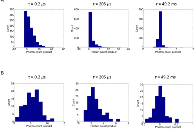
TACF using increasing block-times. The distribution of the block-transformed photon-count products approaches the distribution of the TACF asymptotically as the block-time increases because the TACF corresponds to the block-transformed photon-count product with the maximum possible block-time (block number = 1). When the block-time is short, however, the distributions of the transformed photon-count products are not normally distributed due to the Poisson statistics of both the photon detection process and the occupation number of particles in the focal volume (Fig. S1A). As the block-time increases, the distributions become normal, as predicted by the central limit theorem (Fig. S1B), and assumed in Eq. 4 for the noise in the TACF. Note that the use of Eq. 13 to estimate the covariance matrix in the normal noise model (Eq. 4) only requires the samples to be independent, but not necessarily normally distributed.
Figure S1 Analysis of the distribution of noise in the TACF using the block-transformation. (A)
Distributions of the block-transformed photon-count products at three different lag-times (τ = 0.2 μs, 205 μs, 49.2 ms) are calculated from a simulated photon-count trace with block-time 26.4 ms. The photon-count trace is simulated for two-component diffusion with the same simulation parameters as in Fig 2B except for the simulation time of 26.4 sec. (B) Distributions of the block-transformed photon-count products calculated from the same simulated photon-count trace with block-time of 264 ms. As shown in Figure 4A, the distributions in S1A and S1B are both generated from independent samples.
likelihood estimate and a low dimensional shrinkage target with an optimal shrinkage weight associated with the specific shrinkage target. For covariance estimators, the high dimensional maximum likelihood estimate is the sample covariance, and the low dimensional shrinkage target can be a diagonal matrix. A good choice of the shrinkage target should yield the shrinkage estimate with the structure close to the expected structure. To choose the optimal shrinkage target for covariance estimates of noise in TACFs, we explore different shrinkage targets that preserve the characteristic structure of the noise covariance in the TACF1, 2. For target B and D, the shrinkage estimate of the covariance is given by Eq. 8. Target B is a uniform diagonal matrix with the matrix element and its associated shrinkage weight given by
E if
0 if (1)
∑ Var,
∑ ∑ (2)
where s is the matrix element of the sample covariance matrix S; E and Var denote the sample mean and variance respectively. Target D is the non-uniform diagonal matrix of the variance:
if
0 if (3)
∑ Var
∑ . (4)
Target D shrinks the covariance but preserves the variance. In contrast, the “two-way” target shrinks the variance and the correlation individually. The matrix element of the shrinkage estimate with the “two-way” target is given by
where 1 (6) · 1 (7) min 1,∑ Var ∑ (8) min 1,∑ ∑ Var (9)
and is the matrix element of the sample correlation matrix. We examine structures of regularized correlation matrices and the performance of Approach 2 with different shrinkage targets when the underlying photon-count trace is short (Fig. S2). We choose the “two-way” target for the current procedure because it preserves the correlation structure and yields smaller uncertainty in model probabilities at the same time.
(D) (E)
Figure S2 Comparison of shrinkage estimators for covariance with different targets. (A) Top:
sample correlation matrix of noise in the TACF for two-component diffusion with parameters
kappa = 0.01, 2
1 270 / sec
D m , 2
2 27 / sec
D m , and T 26.4 sec. The covariance matrix is estimated from 1005 independent photon-count products after blocking transformation. Bottom: noise correlation matrices given by different shrinkage estimators for the TACF calculated from only the first 1/80 of the same photon-count trace, which gives 11 independent photon-count products after blocking transformation. (B-E) Model probabilities as a function of acquisition time calculated using Approach 2 with different covariance estimates: (B) “two-way” target (C) diagonal only (variance) (D) target D (E) target B. In all cases, medians and upper and lower quartiles are shown for the eight individual curves analyzed for each data point.
volume is implemented according to Wohland et al., 2001. Briefly, diffusion of a fixed number of particles corresponding to approximately 1 nM concentration ( 69 is simulated using a random walk in a sphere of 3 µm radius. A new particle is placed at a random position on the surface of the sphere when a particle leaves the sphere in order to maintain constant number density. The step size of the random walk in each Cartesian coordinate direction is given by , where is the particle diffusion coefficient, is a normally distributed random number with unit variance and zero mean, and Δ is the size of the time-step (0.2 μs). Fluorescence excitation by a microscope objective of 63x magnification and 1.2 numerical aperture (NA) is simulated assuming a Gaussian Laser Beam (GLB) profile3, with laser power P (100 µW), wavelength (514.5 nm), and characteristic beam width of 261 µm. Fluorescence emission is simulated accounting for the actual position of the particle in the focal volume, its absorption cross-section ( ), and its fluorescence quantum yield (0.98). The emission photon count for a particle at from the center of the sphere is thus
given by , where is the GLB profile in cylindrical
coordinates. Effects of photobleaching, saturation, and the triplet state of the fluorophore are ignored in the current simulation.
The mean number of collected photons from a particle depends on the Collection
Efficiency Function (CEF) of the pinhole4, 5 through , where
is a constant representing the ambient light, and and were defined above.
for a pinhole with diameter of 50 μm is calculated by numerical integration according to Rigler et al. 19935. For all simulations in this work, and if not otherwise specified.
is used except for the simulation for varying , in which a constant corresponding to a count rate of 5 kHz is used to avoid zero correlation at low . and 0 of the focal volume, or MDF, are obtained by fitting a 3D-Gaussian function to the resulting MDF, which is given by
. The simulation is implemented in MATLAB (The MathWorks,
(i1, 2, 3) 2 i x D t D abs 2.2 10 m 20 2 f q e N
r, z
I , e phot abs f N r z e t q I , z
r CEF( , ) D e D bg N N r z q N bg N q
D CEF( , )r z 0.01
qD0.25 0 bg N Nbg
MDF( , ) CEF( , ) I( , )r z r z r zparticle is ~ 35 kHz, which is within the typical range of count rates of fluorophores 20-60 kHz. TACF curves are computed using the multi-tau algorithm6, which has 128 channels recording fluorescence intensities with a quasi-logarithmic scale time increment; namely, the time increment is doubled after the first 16 channels and then doubled every 8 channels. The counts in two adjacent channels are summed before being passed to the next channel with double time increment (see Wohland et al. 2001 for details).
S4 Nonlinear regression and calculation of model probabilities
The noise covariance matrix in Eq. 4 is estimated from multiple independent TACF curves or from the blocked-transformed photon-count products using the regularized shrinkage estimator with the “two-way” target2 (Fig. 1, Supporting Information S2). In the current work we employ a uniform parameter prior ; therefore and are equivalent to and , which can be computed using standard nonlinear regression algorithms.. Generalized least squares regression with is performed using the MATLAB function nlinfit, which employs the Levenberg–Marquardt algorithm to implement a nonlinear least squares regression assuming uniform, independent error terms, thereby minimizing . To adapt this approach to handle correlated noise, we note that the negative logarithm of Eq. 4 is
proportional to , which can be written as
, where is given by the Cholesky decomposition of the covariance matrix 7. The regression problem can then be transformed to an ordinary least squares problem with the transformed data vector and the transformed vector of the function values , which can be solved using the MATLAB function nlinfit. All TACFs are fit with the FCS models defined in Eq. 2 and 3 with an additional constant term to account for the random fluctuation in about zero due to finite acquisition time. The best-fit estimate and the covariance matrix of the parameters are then used to compute the model probabilities using Eq. 6. The prior probability is taken as a constant that is normalized
C
( , k)
P β M βˆBayes Bayes βˆMLE
MLE C 2 [ i ( , )]i i y f x
β T 1 [y f( , )]x β C y[ f( , )]x β
T 1 1 [y f( , )]x β L TL y[ f( , )]x β L T C LL 1 L y 1f( , ) L x β G ˆ MLE β MLE ( , ) P β Mdeviations are estimated as the square root of the diagonal terms of . is chosen to be 200 so that the prior range is significantly larger than the range of parameters suggested by the MLE. The effect of different choices of prior on model probabilities was examined in detail in8. Once has been computed for each model, the normalized model probability is given by
assuming uniform model priors .
Bayes Σ
f ( k) P y M 1 ( k ) ( k) / d ( k) k P M y P y M
P y M P M( k)(B) (C)
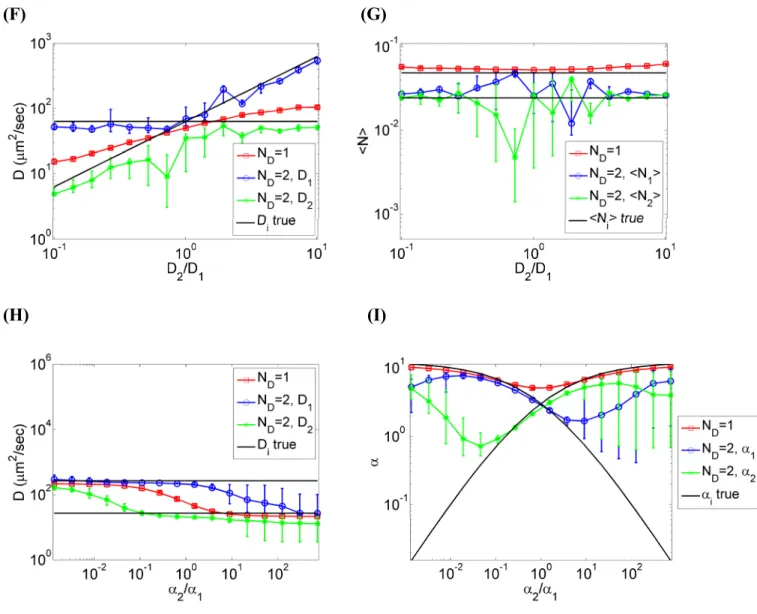
Figure S3 Parameter estimates from the Bayesian analysis of simulations in Fig. 3A-D using
Approach 1 (GLS fitting). In all cases, medians and upper and lower quartiles are shown for the eight mean curves analyzed for each data point.
Figure S4 Bayesian analysis of the same simulations as in Fig. 3A-E using Approach 1 without
incorporating noise correlations (WLS fitting). In all cases, medians and upper and lower quartiles are shown for the eight mean curves analyzed for each data point.
(B) (C)
(H) (I)
Figure S5 Parameter estimates from the Bayesian analysis of simulations in Fig. S4 using
Approach 1 without incorporating noise correlations (WLS fitting). In all cases, medians and upper and lower quartiles are shown for the eight mean curves analyzed for each data point.
(C)
Figure S6 Bayesian analysis of simulations for two-component diffusion with varying
simulation parameters using Approach 2 (GLS fitting). All the simulation parameters are identical as in Fig. 3 except that each curve has simulation time 26.4 sec; thus overall simulation times are the same as in Fig. 3. In all cases, medians and upper and lower quartiles are shown for the eight individual curves analyzed for each data point. The top panel in (B) shows the ratio of sample size and the dimension (n p/ ) for the covariance estimate.
(B) (C)
(D) (E)
Figure S7 Parameter estimates from the Bayesian analysis of simulations in Fig. 4C, 4D and
S6A-C using Approach 1 (GLS fitting). In all cases, medians and upper and lower quartiles are shown for the eight individual curves analyzed for each data point.
Figure S8 Bayesian analysis of the simulations in Fig. 4C, 4D and S6A-C using Approach 2
without incorporating noise correlations (WLS fitting). In all cases, medians and upper and lower quartiles are shown for the eight individual curves analyzed for each data point.
(B) (C)
(H) (I)
Figure S9 Parameter estimates from the Bayesian analysis of simulations in Fig. S8 using
Approach 2 without incorporating noise correlations (WLS fitting). In all cases, medians and upper and lower quartiles are shown for the eight individual curves analyzed for each data point.