Dynamic Pricing: A learning Approach
Texte intégral
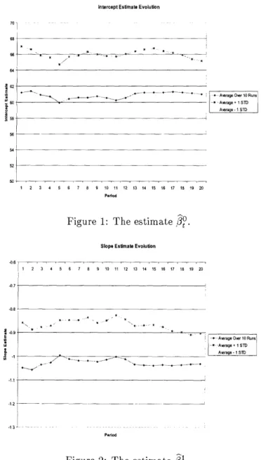
Figure
Documents relatifs
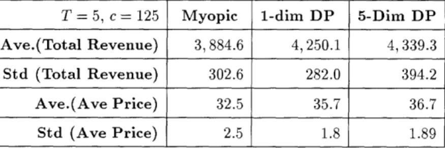
Each time the optimization problem has been solved, all pricing policies obtained from the four models have been recorded and compared with the pricing policy found by the
In a competitive environment, we consider the problem faced by a service firm that makes decisions with respect to both the location and service levels of its facilities, taking
In a competitive environment, we consider the problem faced by a service firm that makes decisions with respect to both the location and service levels of its facilities, taking
Keywords— Quantitative finance, option pricing, European option, dynamic hedging, replication, arbitrage, time series, trends, volatility, abrupt changes, model-free
In this section we establish the link between the viability kernel and the zero level set of the value function of a related Dynamic Programming (DP) problem.. Consequently,
To illustrate the price endogeneity effect caused by model misspecification, we specifi- cally consider a dynamic pricing setting where the true demand model is
simultaneous dynamic pricing can result in revenue gains of between 5 and 7 per cent over traditional RM when used in a simple network with one airline and two flights.. The
In the other experiments, we will compare the performance of the robust pricing models, using three different types of robust objectives (MaxMin, MinMax Regret, MaxMin Ratio) and
