DNS and LES of turbulent flow in a closed channel
featuring a pattern of hemispherical roughness elements
The MIT Faculty has made this article openly available. Please share how this access benefits you. Your story matters.
Citation Chatzikyriakou, D.; Buongiorno, J.; Caviezel, D. and Lakehal, D. “DNS and LES of Turbulent Flow in a Closed Channel Featuring a Pattern of Hemispherical Roughness Elements.” International Journal of Heat and Fluid Flow 53 (June 2015): 29–43 © 2015 Elsevier Inc
As Published http://dx.doi.org/10.1016/j.ijheatfluidflow.2015.01.002
Publisher Elsevier
Version Author's final manuscript
Citable link http://hdl.handle.net/1721.1/109404
Terms of Use Creative Commons Attribution-NonCommercial-NoDerivs License
DNS and LES of Turbulent Flow in a Closed Channel Featuring a Pattern of Hemispherical Roughness Elements
D. Chatzikyriakou1, J. Buongiorno1*, D. Caviezel2, D. Lakehal1, 2
1 Massachusetts Institute of Technology, 77 Massachusetts Avenue,
Cambridge, MA 02139, USA
2 ASCOMP GmbH, Zurich, Switzerland
Corresponding Author: * jacopo@mit.edu
ABSTRACT
Direct Numerical Simulations (DNS) and Large Eddy Simulations (LES) were performed for fully-developed turbulent flow in channels with smooth walls and walls featuring hemispherical roughness elements at shear Reynolds numbers Reτ = 180 and
400, with the goal to study the effect of these roughness elements on the wall-layer structure and on the friction factor. The LES and DNS approaches were verified first by comparison with existing DNS databases for smooth walls. Then, a parametric study for the hemispherical roughness elements was conducted, including the effects of shear Reynolds number, normalized roughness height (k+=10-20) and relative roughness spacing (s+/k+=2-6). The sensitivity study also included the effect of distribution pattern (regular square lattice vs. random pattern) of the roughness elements on the walls. The hemispherical roughness elements generate turbulence, thus increasing the friction factor with respect to the smooth-wall case, and causing a downward shift in the mean velocity profiles. The simulations revealed that the friction factor decreases with increasing Reynolds number and roughness spacing, and increases strongly with increasing roughness height. The effect of random element
distribution on friction factor and mean velocities is however weak. In all cases, there is a clear cut between the inner layer near the wall, which is affected by the presence of the roughness elements, and the outer layer, which remains relatively unaffected. The study reveals that the presence of roughness elements of this shape promotes locally the instantaneous flow motion in the lateral direction in the wall layer, causing a transfer of energy from the streamwise Reynolds stress to the lateral component. The study indicates also that the coherent structures developing in the wall layer are rather similar to the smooth case but are lifted up by almost a constant wall-unit shift y+ (~10-15), which, interestingly, corresponds to the relative roughness
k+=10.
I. Introduction
The effect of wall roughness on the structure of the wall boundary layer has always been a subject of dedicated research, since the pioneering work of Colebrook [1] and Nikuradse [2]. An abundant literature is available for single-phase, turbulent flow in channels with large roughness elements of various shapes – see for instance the review of experimental work provided in Ref. [3]; however, there is little to cite as to the effect of small hemispherical roughness elements regularly or randomly distributed on the channel wall; a situation that is relevant to various energy systems such as fossil boilers and nuclear reactors, in which vapor bubbles are attached to the wall in subcooled flow boiling and effectively behave like small (<100 µm), near-hemispherical, roughness elements. The objective of this study is to investigate the effects of small solid hemispherical roughness elements on fully developed turbulent channel flow by using high-fidelity DNS and LES simulations. In particular, the effect
of shear Reynolds number, roughness size, spacing and distribution (random vs. regular pattern) for roughness elements is explored here in a systematic way.
The size and distribution of the hemispherical roughness elements studied here are informed by the subcooled flow boiling situation in the hot fuel assembly of a Pressurized Water Reactor (PWR). However, here there is no intent to simulate actual bubbles, only small solid hemispherical roughness elements.
Background and a brief literature review are given in Section II. The numerical procedure is described in Section III. The DNS and LES studies for smooth wall channel flow and one representative case with hemispherical roughness elements are presented in Section IV. A parametric LES analysis for hemispherical roughness elements is presented in Section V. The conclusions and recommendations for future work are discussed in Section VI. The LES quality and solution verification are reported in the Appendix
II. Background
The introduction of high fidelity simulation approaches and ever more powerful computers has allowed a series of DNS studies of fully developed flow over rough-walled rectangular channels with two dimensional ribs, with detailed PIV data [4, 5] for model validation. In most of these studies, the ribs were quite large, reaching up to 20% of the channel half height. The effect of rib spacing was studied widely with DNS and LES [6] [7] [8] [9] [10] [11], and resulted in a classification of the flow behavior based on the height-to-spacing ratio of the ribs. One of these studies dealt with the effect of uneven rod height [9]. Refs. [12] and [13] report on the effect of randomly distributed height of 2D roughness elements. 3D roughness elements were
studied as well with DNS [14] [8, 15-17], including the effects of the Reynolds number and the spacing between elements.
However, numerical data for small roughness elements are limited. The numerical study presented in this paper investigates fully-developed turbulent flow over small hemispherical roughness elements at high Reynolds number; here ‘small’ means that the size of the roughness elements is of the order of the near-wall viscous boundary layer, which of course decreases at increasing Reynolds number. Data so obtained fill the gap between the smooth-wall data and other large-roughness results abundant in the literature. The availability of high performance computing facilities lifts the obstacle of inadequate resolution of the small roughness elements.
The interaction between the roughness elements attached to the wall and the streamwise vortices modifies the near-wall layer with respect to the case of a smooth-wall flow. The effect of roughness elements on the velocity profile can be described by means of the following formalism.
The velocity defect, defined as the difference between the mean velocity and the
centerline velocity can be normalized by u (shear velocityu w
) and correlated
only to y u y (
is the kinematic viscosity), according to the following equation:
1 ln
U y A
(1)
where is the von Karman constant (~0.4) and A is the smooth wall constant (A~5.1 for flow in a pipe). The + symbol indicates normalization. In the rough wall regime,
the velocity profile in the inner layer would be modified according to the following equation:
1 1 ln y , ln U B k B k A U k k (2) U is the modification of the smooth wall constant due to roughness effects and is frequently called the roughness function. k is the wall-normal height of the roughness
elements in meters. The shear Reynolds number is given as: Re hu
, where h is the
half channel height. Also the friction coefficient is defined as:
2 2 8 8 w b b u f U U (3)
where Ub is the bulk fluid velocity.
III. Numerical Procedure
A. Computational algorithm
The three-dimensional DNS and the LES simulations presented here were performed with the finite volume CFD/CMFD code TransAT©. A collocated, Cartesian grid was used and the incompressible Navier-Stokes equations were solved. The approach employed here is to represent the solid obstacles in a Cartesian mesh (rather than using a body-fitted grid). The method used [18] is a specific variant of the Immersed Boundary Method of Peskin [19, 20]. In the present Immersed Surface Technique (IST), the solid object is captured in the Cartesian grid using a level set function; where the positive values denote the fluid domain, the negative values identify the solid domain and the surface of the wall is implicitly represented by the zero level set. The fluid domain indicator function (derived from the level set function) varies smoothly across the wall surface with a support of two cells on each side of the fluid-solid interface. The no-slip condition at the wall is imposed through a relaxation term
which acts as a distributed momentum sink reducing the fluid velocity as the indicator function goes to zero [21].
The mesh was locally refined in the regions of interest, namely in the region right next to the walls extending into the wall-normal direction beyond the end of the roughness elements and up to the buffer layer. In those regions, the grid had two layers of ghost cells enabling the high resolution of the roughness elements (~10 grid points per element radius). Then, the meshed domain was decomposed into a number of blocks equal to the number of processors to be used for the calculation. Transfer of information between neighboring blocks was performed using MPI parallelization. All simulations were carried out using the 2nd order Central Difference scheme for the discretization of the convective fluxes. An explicit 3rd order Runge-Kutta scheme was used for the time integration. The time-step was adaptive and bound by a Courant number fixed between 0.1 and 0.3 to guarantee stability of the simulations. For the pressure-velocity coupling the SIMPLEC algorithm was used. The SIP preconditioned GMRES augmented by the use of the parallel PETSc solver library was used for the pressure solver.
In the LES simulations, the WALE subgrid scale model [22] was used to account for the unresolved, subgrid-scale turbulence. This is a zero-equation model with features similar to Smagorinsky’s model [23][24], albeit including the rate of change of vorticity in the definition of the eddy viscosity, besides the strain rate tensor.
All simulations were set up and post-processed on a local, 64 bit, 12-core workstation machine and run on hundreds or thousands of MPI-enabled processors in the Oak Ridge Leadership Computing Facility ‘Jaguar’, now called ‘Titan’.
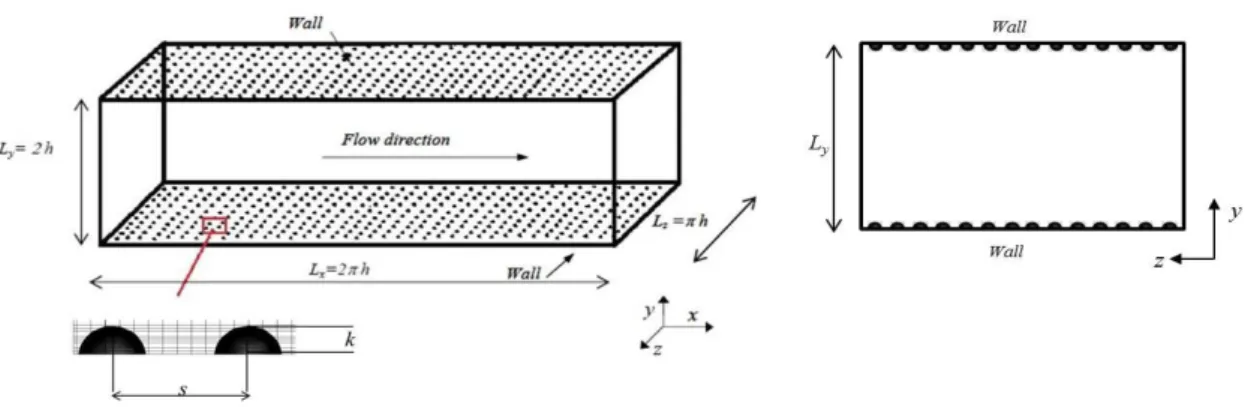
In all simulations the domain consisted of a Cartesian box (Figure 1), the size of which was selected to include the largest eddies in the flow and such that the turbulent eddies would not be correlated. Thus, for the smooth wall flow the Cartesian box had dimensions Lx = 2πh, Ly = 2h, and Lz =πh, where h is the half-channel height (wall-normal direction). h was kept constant in all our simulations. The streamwise and spanwise dimensions of the box were varied slightly between simulations in order to account for the different number of roughness elements or the increase or decrease in the spacing between roughness elements. Since fully developed turbulent channel flow is homogeneous in the streamwise and spanwise directions, x and z respectively, periodic boundary conditions could be applied in these directions. No-slip boundary conditions were applied both on the upper and lower horizontal planes of the channel and on the roughness elements surface.
Figure 1. Schematic of computational domain for roughened-channel flow simulations
The shear Reynolds number Reτ was set at 400 and 180. A pressure gradient source
term was imposed in the x-momentum equation in order to achieve the imposed shear velocity, and thus the target shear Reynolds number. The shear velocity relates to the pressure gradient (dp/dx) in the following way:
1/2 h dp u dx (4)
For the coarsest LES simulation of rough wall channel flow, the flow field was initialized using a previously-run fine grid LES simulation of smooth turbulent channel flow with the same shear Reynolds number (Reτ=400 or 180 respectively).
For all subsequent simulations of rough wall channel flow, both LES and DNS, the coarsest rough-wall LES simulation velocity and pressure fields were used to initialize the flow field.
Turbulent statistics were computed from solution samples, once statistically ergodic conditions were obtained. Space averaging was also performed in the streamwise and spanwise directions throughout the entire domain. More details are given separately with the presentation of each case.
IV. Simulations
A. Overview
The following sequence of simulations and analyses was performed:
1. Smooth wall LES and DNS, including solution verification and validation.
2. LES of one representative hemispherical element case, including solution verification.
3. DNS simulations of one representative hemispherical element case.
4. Comparison of LES and DNS for the representative hemispherical element case. 5. LES parametric study for hemispherical roughness elements, with variation of the
spacing between hemispheres, hemisphere height and Reτ. LES with random
The simulation matrix is reported in Table I.
Table I. Simulation matrix of LES and DNS cases Smooth
Wall
Wall with Hemispherical Roughness Elements
Regular distribution Random
distribution Simulation
type DNS LES DNS LES
roughness size (k+) N/A 10 10 10 10 10 20 10 10 - 20 spacing/size (s+/k+) 2 2 2 4 6 2 2 2 Reτ 400, 180 400, 180 400 400 400, 180 400 400 400, 180 400 400
B. DNS and LES of turbulent flow in smooth channel 1. DNS of smooth channel flow
Three DNS simulations were performed with increasingly finer meshes. The geometry and the boundary conditions are those described above in Section III.B, identical in all three simulations. The streamwise and spanwise spatial discretization was uniform throughout the domain. However, the grid was refined near the wall in the wall normal direction. The minimum and maximum grid-cell values expressed in
h
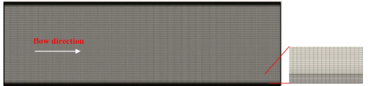
units can be seen in Table II. A typical grid for these DNS simulations can be seen in Figure 2. The refinement ratio between two consecutive grids is (=42),
applied uniformly in the domain. The same scaling applies to both the number of processors used and the total number of cells for each simulation.
Figure 2. Typical grid used for the DNS and LES smooth wall simulations flow direction
Turbulence was established relatively quickly; statistically steady (ergodic) conditions were reached before the collection of statistics started from individual flow fields for the total number of non-dimensional time steps (
2
tu
t
) reported in the bottom row
of Table II. Space averaging was performed in the homogeneous streamwise and spanwise directions in order to increase the statistical sample.
Table II. Simulation characteristics and statistics collection parameters for DNS
simulations of smooth wall channel flow
Grid 1 'vc' Very coarse Grid 2 'c' Coarse Grid 3 'f' Fine Number of nodes x 256 304 362 y 192 228 272 z 192 228 272 Resolution x 9.81 8.18 6.92 min y 0.91 0.76 0.67 max y 5.65 4.71 4 z 6.54 5.45 4.65 Number of processors 480 800 1344 Number of cells (M) 9.3 15.6 26.3
Statistically steady state
after (t+) 12,000 18,000 16,800
Averaging performed
after steady state for (t+) 10,800 10,000 7,200
The mean streamwise velocity for all three DNS cases is presented in Figure 3. The streamwise wall-normal, spanwise and shear stresses are plotted in Figure 4, which also includes two sets of DNS data: those of Krogstad et al. [5] for the same shear Reynolds number and those of Hoyas and Jimenez [25] at Re=550. It can be seen
that the present DNS are in accord with the selected sets of published DNS, for the same order of shear Reynolds number.
Figure 3. Mean streamwise velocity from smooth wall DNS simulations (Re 400).
Figure 4. Streamwise, wall-normal, spanwise and shear stresses from smooth wall DNS simulations (Re 400).
2. LES of smooth channel flow
The LES equations are well known and so is the subgrid-scale (SGS) stress definition and modeling within the eddy viscosity context, linking linearly the SGS eddy viscosity to the gradients of the filtered velocity field. The WALE SGS model [22] was employed in the present context; it defines the SGS eddy viscosity as follows:
3/ 2 2 5/ 4 5/ 2 d d ij ij t w d d ij ij ij ij S S v C S S S S (5) where, 2 10.6 w s C C and Sijd reads:
2 2
2 2 1 1 2 3 d ij ij ji ij kk i ij ij ik kj j S g g g du g and g g g dx (6)where ij is the Kronecker symbol. In the current simulations, the Smagorinsky constantCS is assigned the value of 0.08, and the filter width is set equal to2grid. The model has been shown to behave very well in wall-bounded flows, without a specific damping function similar to Van Driest’s [26]. It has also been shown to be less dissipative and able to capture the thin-shear layer accurately.
Three LES simulations were performed with increasing mesh refinement. The geometry and the boundary conditions shown in Figure 1 were used also for these LES simulations. The grid was refined near the wall in the wall normal direction. The refinement ratio between two consecutive grids was = 2, applied uniformly in the domain. The simulation setup and statistics are presented in Table III. The number of grid points was obviously lower than DNS, however the grid resolution near the wall approached that of the DNS.
Table III. Simulation characteristics and statistics collection parameters for LES
simulations of smooth wall channel flow
Grid 1 'vc' Very coarse Grid 2 'c' coarse Grid 3 'f' Fine Number of nodes x 91 128 181 y 68 96 136 z 68 96 136 Resolution x 27.74 19.61 13.87 min y 2.56 1.81 1.28 max y 16.00 11.31 8.00 z 18.48 13.07 9.24 Number of processors 24 60 168
Number of cells (Million) 0.4 1.2 3.3
Statistically steady state
after (t+) 40,000 20,000 12,000
Averaging performed
after steady state for (t+) 24,400 18,400 10,800
The mean streamwise velocity for all three LES grids is presented in Figure 5, along with the streamwise wall-normal, spanwise and shear stresses in Figure 6. For comparison, the figures also report our DNS results. Note that the LES solution approaches the DNS solution as the mesh is refined, which is the expected behavior. The accuracy of the LES was high even at low grid resolutions, as it predicted both the mean velocity and the stresses distributions well. The mean streamwise velocity value at the center of the channel had maximum and average deviations from the DNS solution of 3.5% and 1%, respectively. The convergence and the quality of the LES simulations are discussed in the Appendix.
Figure 5. Mean streamwise velocity profile from smooth wall LES simulations, compared to DNS of the same case (Re 400).
Figure 6. Streamwise, wall-normal, spanwise and shear stresses from smooth wall LES simulations, compared to DNS of the same case (Re 400).
C. DNS and LES of channel flow with hemispherical roughness elements
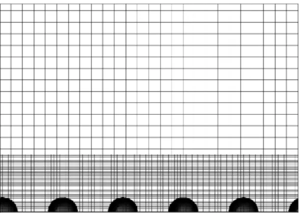
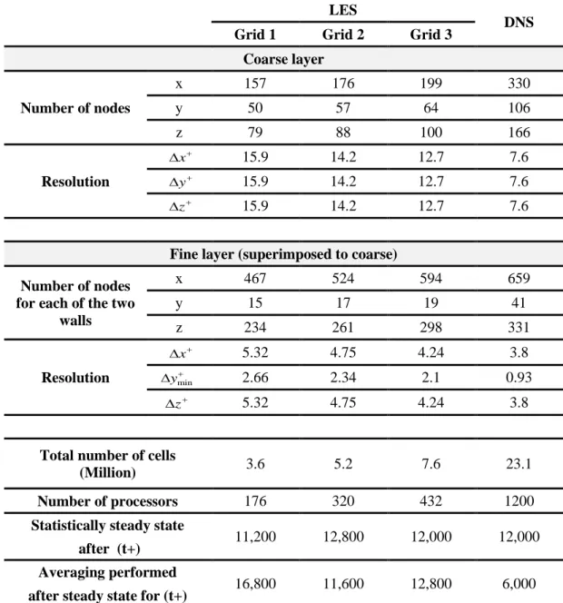
One DNS and three LES simulations of the turbulent channel flow case with hemispherical roughness elements were performed. The geometry and boundary conditions are those shown in Figure 1. The BMR (short for Block Mesh Refinement) technique was used in all hemispherical roughness elements cases to resolve the wall layer containing the roughness elements in order to alleviate the resolution limitations of simple, single-block refined grids as used in the smooth cases (Figure 2). The BMR gridding is shown in Figure 7. A uniform coarse grid was used as the first layer and a refined grid was superimposed to that first layer covering the region starting from the wall and up to y+~40 (applied to both walls). The refined layer featured a gradually decreasing resolution in the y-direction while in the x- and z directions the resolution was fine yet uniform.
Figure 7. Block Mesh Refinement (BMR) technique used for rough wall LES and
DNS simulations.
Beyond y+~40 the resolution is decreased towards the center of the channel with the mean grid size increasing from the near wall region (min 2.4-DNS case) to the mid channel plane (max 7.6-DNS case). Both the minimum and the maximum mean grid
sizes satisfy the criterion for sufficient grid resolution [27]. That criterion dictates that the average should be lower than . In our case, the non-dimensional Kolmogorov lengthscale was + ~ 4.5. The simulation characteristics along with the
averaging details and the statistics are reported in Table IV both for LES and DNS.
Table IV. Simulation characteristics and statistics collection parameters for DNS and
LES simulations of hemispherical roughness channel flow (using the BMR meshing method)
LES DNS
Grid 1 Grid 2 Grid 3
Coarse layer Number of nodes x 157 176 199 330 y 50 57 64 106 z 79 88 100 166 Resolution x 15.9 14.2 12.7 7.6 y 15.9 14.2 12.7 7.6 z 15.9 14.2 12.7 7.6
Fine layer (superimposed to coarse) Number of nodes
for each of the two walls x 467 524 594 659 y 15 17 19 41 z 234 261 298 331 Resolution x 5.32 4.75 4.24 3.8 min y 2.66 2.34 2.1 0.93 z 5.32 4.75 4.24 3.8
Total number of cells
(Million) 3.6 5.2 7.6 23.1
Number of processors 176 320 432 1200
Statistically steady state
11,200 12,800 12,000 12,000
after (t+) Averaging performed
Space averaging is performed over the entire domain, both in x and z directions while
the regions obstructed by the hemispheres are excluded. Therefore, a single, representative y-distribution for velocity and Reynolds stress can be extracted. However, it is interesting and important to analyze also the flow structure locally, in the vicinity of the hemispherical roughness elements. Data was extracted from our DNS simulation results for several x-z locations, as shown in Figure 8. Position A in the sketch corresponds to the top of the obstacle whereas all other positions were taken in between obstacles.
Figure 8. Locations of data extraction on x-z plane.
The data extracted were the mean velocity profiles (only time averaged) in the y-direction, and are shown in Figure 9, using inner scaling. Note that the mean velocity profiles for the cases with hemispherical obstacles, a downward shift from the smooth wall solution was observed, since the drag created by the obstacles slows down the flow (for the same imposed pressure gradient). The shift was constant in the outer flow region (U+~2), which was way lower than what has been observed in other
inspection of the profiles suggested that this behavior was clearly dependent on the sampling location: while right at the top of the elements, the shift was complete, in-between locations (B, C, D) the flow exhibited transition mechanisms from smooth to rough scenario, with a gradual destruction of the viscous sublayer. It is noted that in
Figure 9, the origin of y+ (or point where y+ is 0) is always the boundary corresponding to the wall without the obstacles. As a result, the curve corresponding to point A starts from y+=10.
Figure 9. DNS Mean velocity profiles for s/k=2 for the locations shown in Figure 8. Comparison with smooth wall velocity profile and law of the wall.
On average, the velocity profiles should exhibit a roughness-induced structure similar to that of Figure 10. The streamwise mean velocity profiles obtained with both LES and DNS are presented in Figure 10 against wall units, and are compared to the
log-law. The normal and shear stresses are plotted in Figure 11, using outer scaling (y/h), which is the practice for grid and model convergence studies. As expected, the LES
solution approached indeed the DNS solution as the mesh was refined. The accuracy of the LES was rather high for such a complex geometry even at low grid resolutions (comparing to DNS; 7.6 million cells vs. 23 million cells; actually convergence was already attained for Grid 2 LES); both the mean velocity and the stresses were well predicted. The profiles clearly depicted a drag enhanced flow induced by the presence of the roughness elements, eliminating the viscous-layer flow features (y+ < 11.6) from the picture.
Figure 10.Mean streamwise velocity profiles for LES simulations of hemispherical roughness case, compared with DNS of the same case.
Figure 11. Streamwise, wall-normal, spanwise and shear stresses profiles for LES of
hemispherical roughness case, compared with DNS of the same case.
Let us now turn to the comparison of the smooth and rough cases. For this purpose we used the finest LES grid (Grid 3) results only. While it was clear that the inner scaling applied to the mean velocity profile exhibited a downward shift, it was interesting to address the universality of that shift and its dependence on the roughness elements. The mean velocity defect can be expressed as U+= (U+ - UCl) where UCL is the
centerline velocity. When plotted in outer scaling (vs. y/h), U+ for Re=400 showed a perfect overlap in the outer flow region (Figure 12a), meaning that either the shift function is universal or the velocity characteristics were independent of surface geometry in the outer region, which is consistent with Townsend’s [28] Reynolds number similarity hypothesis. Inner scaling (Figure 12b), however, suggests that the shift function is not universal in the inner layer. We thus concluded that the Reynolds
number similarity hypothesis could be justified only in the outer layer, and thus the velocity characteristics were somewhat dependent on the surface topology.
(a)
(b)
(a) Plots in outer scaling
(b) Plots in inner scaling
Figure 13. Streamwise, wall-normal, spanwise and shear stresses profiles for LES and
While the outer-scaling plots of the stresses (Figure 13a) did not show substantial differences, the inner-scaling plots revealed some interesting findings as to the effect of roughness on turbulence, interpreted broadly (Figure 13b). The vertical fluctuating stresses seemed to be unaffected by the presence of roughness elements. The fluctuating field decayed as the wall (smooth or rough) was approached in a similar way. The most important finding was that the rate of momentum transfer from the mean flow to the streamwise fluctuating field, and thus <u’2> reduced in effect compared to the smooth case by about 10%, with the peak location sliding towards the outer layer by about y+=10. Conservation of momentum and energy requires that the losses be absorbed by another component: the <w’2>. The peak location for this
quantity was now shifted back. Below y+=11, all energy components were drastically weaker than in the smooth case, apart from the vertical stress, where the similarity of the decay of turbulence was clearly independent of the surface topology.
Also, the turbulent kinetic energy (TKE=1/2 (<u’2>+<v’2>+<w’2>)) profiles for the
case of hemispherical roughness elements and the smooth wall case can be seen in
Figure 14. The TKE levels were lower near the wall for the rough case, while they
did not seem to differ in the middle of the channel. That is due to the flow slowdown in the streamwise direction. This means that there was a clear cut between the inner and outer layer in this case, a feature observed also with other types of roughness elements [5, 15]. The behavior of TKE is in fact similar to the streamwise stress component, which contributes most to TKE.
Figure 14.Turbulent kinetic energy distribution in the spanwise direction for rough and smooth wall DNS.
The sources of energy transfer between the three turbulent stress components can only be revealed through a detailed analysis of the source terms in the Reynolds stress budget. Looking solely at the production of turbulence kinetic energy term may be either misleading in the 3rd direction-flow-homogeneity assumption or may hide other
important subtle mechanisms.
The pressure diffusion source term provides a better and more straightforward way to explain the inter-component energy redistribution observed in Figure 13. The term provides a source of energy and a contribution mechanism to redistribute it. The energy redistributive part called the pressure-rate-of-strain tensor and defined as [29]
j i ij j i u u p R x x (7)
serves in effect to redistribute energy among the Reynolds stresses promoting isotropy of turbulence. By virtue of continuity, the trace of Rij is zero, and consequently this
term vanishes in the transport equation of the turbulent kinetic energy. Each term of the trace of Rij is then used to define the pressure–strain correlation,
i ii i u p R x (8)
a positive value of which implies a transfer of energy into component i from the other components, and vice versa. The transfer of energy from <u’2> to <w’2> observed in
Figure 13 can only by explained by R33 being > 0, reflecting the occurrence of local, instantaneous bulging flow in the third direction induced by the roughness elements,
thus w 0 z .
Contours of the instantaneous streamwise velocity in the entire domain are shown in
Figure 15Error! Reference source not found.a while Figure 15Error! Reference
source not found.b shows the instantaneous velocity contours at a slice in the middle of the hemispheres, as those where computed from the DNS simulation. The recirculation regions in between the hemispheres are also featured in the same figure. The flow was shown to penetrate the roughness layer with negative momentum sucking towards the wall, thus inducing inter-element flow recirculation.
(a) (b)
Figure 15. (a) Instantaneous streamwise velocity contours for slices at the
hemispheres crest and in between hemispheres. (b) Instantaneous velocity contours at a slice in the middle of the hemispheres. The recirculation regions in between the hemispheres can be clearly seen.
A further insight into the wall layer and the effect of the wall roughness on the flow structure could be gained by looking at the instantaneous flow structures in the vicinity of the roughness zone. Figure 16 compares the patchy quasi-coherent structures in the smooth case and rough case (for k+= 10 and s+=2) at different heights from the wall: at y+=5, 10, 15, 20, 25 and 30. Unlike previous similar studies, where the large square obstructions placed perpendicular to the flow direction caused large differences between the smooth and the rough wall flow structures [10], here we observed one important phenomenon worth reporting, that is: the coherent structures controlling the drag were rather similar to the smooth case (at least for this roughness configuration, spacing and height) but were lifted up by almost a constant wall-unit shift y+ (~10-15), which, interestingly, corresponds to the relative roughness k+=10.
Figure 16. Smooth wall (left) and hemispherical obstacles wall (right) instantaneous
streamwise velocity contours at various y+ locations from the wall. Planes parallel to the wall.
As explained in Section II, the effect of the roughness elements on the flow is to shift the mean velocity profile by U with respect to the mean velocity profile of a smooth wall.
The friction factor can be extracted from the simulations using equation (3) and then compared to the friction factor estimated from Moody's diagram (or equivalent correlations). In the smooth wall case, the channel Reynolds number was approximately 29,000 (both for LES and DNS with small deviations). For this value of the Reynolds number, Moody's diagram gives a friction factor value of 0.024, whereas our LES and DNS simulations plateaued at 0.025, as shown in Figure 17. The friction factor for the case with hemispherical roughness elements, extracted from the DNS and LES simulations, is shown in Figure 18. It plateaued at about 0.0324, which is higher than the smooth wall case, as expected. The relative roughness (i.e. ratio of height of hemispherical obstacles to the channel hydraulic diameter) is 0.00625 and the Reynolds number is 25,100 for the DNS simulation. For this input, Moody's diagram gives a friction factor of 0.0355. The two values are within 8%, so Moody’s diagram actually does a reasonable job at predicting the friction factor for our hemispherical roughness case. Note that the fine-grid LES simulation predicted a friction factor that is very close to the DNS-predicted value, again confirming the high quality of our LES approach despite the fact that the number of cells is less than 1/3 that of the DNS (LES: 7.6 million vs DNS: 23 millions).
Figure 17. Friction factor as a function of the number of cells for DNS and LES studies for smooth wall case. The solution actually converges at around 10 million cells already.
Figure 18. Friction factor as a function of the number of cells for DNS and LES
V. LES Parametric Study of Hemispherical Roughness Elements Effects
The effect of roughness elements on the mean velocity, wall shear stress and friction factor is expected to depend on the shape, size, pattern and spacing of the elements, as well as on the Reynolds number. There have been several studies in the literature investigating the nature of this dependence. The most relevant ones to our study are summarised in Table V. To the best knowledge of the authors, the present study is one of the few that address the effect of randomness of roughness distribution, and compare it to the case of a square lattice distribution.
To study such effects parametrically, the simulations summarized in Table VI were performed using the LES approach. The reference case described in the previous section was used as a baseline for comparison. The mesh used in all the LES simulations of this parametric study was the same and it was the finest LES mesh used in the analysis in Section III.C, which was proven to return results close to DNS. In this section, the averaging procedure has been performed both in time and in space; the latter was performed throughout the entire domain by averaging the values of the points at the same y-location only. Finally, a time and space averaged velocity was produced starting from the wall of the channel (y+=0), not the top of the obstacles.
Table V. Summary of previous and current work on rough channel flow
k+ h/k Random distribution Shape (2D, 3D) Variable size Simulation type Reτ [5] (Krogstad) 10 29.4 -Square ribs (2D) - DNS 400 [15] (Leonardi) 10 -Square ribs/triangular ribs (2D) - DNS 180, 480, 600 This study 10-20 40 Yes Hemispheres (3D) yes DNS/LES 180, 400
Table VI. Parametric simulation matrix and summary of main findings
smooth hemispherical elements cases
square lattice distribution random lattice roughness size (k+) 10 10 10 20 10 10-20 spacing/size (s/k) 2 4 6 2 2 2 Reτ 400 180 400 180 400 400 400 400 400 Friction Factor 0.025 0.032 0.033 0.035 0.030 0.029 0.044 0.034 0.041 % change from smooth wall case 30 7 21 15 79 37 66 U 3.33 0.9 2.33 1.64 6.11 3.08 5.16 A 4.26 5.05 0.96 4.15 1.93 2.62 -1.85 1.18 -0.9 0.36 0.38 0.34 0.37 0.34 0.35 0.32 0.35 0.33
A. Reynolds number effect
The reference case simulated in Section IV.C had a friction Reynolds number Reτ =
400. To examine the effect of Reynolds number on the flow, we simulated the case of turbulent channel flow with Reτ=180. There is relevant data in the literature for this
value of the Reynolds number and thus we could compare our results to other published data [4,10]. Also, the same grid resolution could be adopted for the lower Reynolds number, without loss of accuracy. We performed this simulation for both smooth and rough wall conditions. The comparison of the mean flow results can be seen in Figure 19. It can be seen that the law of the wall is independent of the Reynolds number for the smooth wall, as expected. For the rough cases, the similarity of the log law is preserved (obviously at y+ > 10) with the same lower velocity defect
U
as compared to the smooth cases (with the slope k remaining roughly unchanged (Table VI)), but with marked deviations in the region very close to the wall (y+ < 10). Both phenomena were explained previously, the lower shift in the core flow region and transition mechanism in the viscous-affected layer. In particular, as the shear
Reynolds number increases, the resistance caused by the roughness elements increases, too, meaning that the flow separates on the roughness surfaces earlier and more abruptly. This is in line with the statement put hitherto: in contrast to square-type of roughness where the flow separates naturally at the edges, in this case there is a Reynolds number effect in the viscosity-affected layer.
Figure 19. Mean streamwise velocity for cases of smooth Reτ=400, smooth Reτ=180,
rough Reτ=400, rough Reτ=180.
B. Size effect
In order to investigate the effect of the roughness size, a case with hemispherical elements of double the size of the reference elements (but with same center-to-center spacing) was simulated. The effect in the downward shift of the mean velocity was significant and the friction factor increased by almost 36% with respect to the reference case (Figure 20). This is consistent with the Moody’s diagram prediction: doubling the roughness increases the friction factor by about 2.5. The main conclusion
to draw here is that increasing the relative roughness k+ shifts the log law further into the core flow.
Figure 20. Mean streamwise velocity for Reτ=400 and two different roughness sizes:
k+=10 and k+=20
C. Spacing effect for regular roughness distribution
The effect of spacing between roughness elements has been studied extensively in the literature, though for square type of roughness mainly. A common classification is that of k-type (‘loose’ spacing) and d-type (‘tight’ spacing) roughness, per Ref. [29]. For k-type roughness, eddies with length scale of order k are shed into the flow above the crests of the elements. For a d-type roughness, stable vortices form within the grooves and there is no eddy shedding into the flow above the elements. Transitional roughness is intermediate between k and d-types [15]. However, this classification was developed for square cross section elements, and may not apply to hemispherical elements for the reasons explained earlier: flow separation is very sensitive and
dependent on the wall curvature. Therefore, the effect of spacing on hemispherical elements was studied for cases with s/k = 2, 4 and 6. The contour plots of the instantaneous velocity for these three cases can be seen below in Figure 21.
The size of these recirculation regions scales with the size of the elements, or the relative roughness. On the other hand, larger spacing seems to enhance momentum transfer from the core flow towards the wall; shorter spacing tends to homogenize the flow in the wall layer.
Figure 21. (left) Time averaged streamwise velocity contour plots and v’ contour
Figure 22. Mean streamwise velocity for Reτ=400 and three different cases: s/k=2, s/k=4, s/k=6.
There was a modest difference between the three cases, with the mean velocity profile (Figure 22) and the friction factor (Table VI) approaching the smooth wall values with increasing spacing, as expected. The log law similarity is perfectly preserved. Unlike d-type square-shaped roughness elements, here for the lowest s/k=2 there was detachment and reattachment of the flow between two adjacent hemispherical obstacles.
D. Effect of random spheres distribution and variable spheres size
The effect of the spatial distribution (pattern) of the roughness elements was also investigated. A random distribution pattern was implemented, with the constraint of a minimum distance between elements of at least s+=20. The instantaneous velocity
contour plot along with the hemispheres distribution can be seen below (Figure 23) for k+=10 and 10<k+<20, while the friction factor is reported in Table VI.
Figure 23. Instantaneous streamwise velocity contour plots for the case of random
spheres distribution. Upper plot: k+=10, Lower plot: 10<k+<20
The turbulent flow field is seen to be well established in both cases, featuring a similar structure to the non-random roughness distribution plotted in Figure 7 above. The details of the flow in the vicinity of the roughness layer cannot be seen. The random distribution has a modest effect on the friction factor, which increases by about 8% as compared to the regular lattice case for the same spacing and Re; by contrast, increasing the relative roughness from 10 to 20 increases the friction coefficient from 0.034 to 0.041, i.e. about 17%, which is not negligible.
Further, the effect of varying roughness elements sizes was also investigated for the (same) random spacing pattern to complete the analysis. The sizes were normally distributed in the range 10<k+<20. The resulting averaged velocity profiles can also
be seen in Figure 24, and again in Table VI as to the friction factor. The value of the friction factor for this case is lower than the case of random large obstacles, as expected. The figure shows that for k+=10, regular versus random roughness distributions present the same behaviour: a downward shift in the velocity profile, retaining the log law structure at the expense of washing out of the viscous sublayer. Increasing the relative roughness to k+=20 shifts further down the preserved log profile away from the wall, at the same time pushing its validity further up; y+> 30.
Figure 24. Mean streamwise velocity for Reτ=400 and four different cases: square pattern with s/k=2 and k+=10 and k+=20, and random lattice with k+=10 and 10< k+<20.
The effect of increasing roughness height elements from k+=10 to k+=20 is seen in
case of k+=10 with a random distribution does not show any difference with the regularly spaced case, and thus it is not included in the graph. As discussed previously in the context of Figure 13, increasing roughness height causes a transfer of energy from the streamwise component to the lateral one; the phenomenon seems to be pronounced with increasing roughness height, but is independent of their distribution.
VI. Conclusions
A detailed simulation campaign based on LES and DNS to investigate of the effect of hemispherical roughness elements on fully developed turbulent flow between parallel plates was presented here. Variations in the shear Reynolds number (Reτ=180-400),
element height (k+=10-20), element spacing (s+/k+=2-6) and distribution pattern (regular square lattice vs. random pattern) were explored to assess their effect on the friction factor and mean velocity and turbulent stresses profiles. The present LES/DNS campaign differs from the abundant published work centering on large sharp-edged roughness obstructions (k+=40-100), in that it deals with the transitional roughness regime, where the Reynolds number is relatively high (for a DNS), and the roughness elements are small and of round shape, and could thus be randomly distributed.
Overall the DNS results show a clear separation between the inner wall-layer, which is affected by the presence of the roughness elements, and the outer layer, which remains relatively unaffected. The roughness element height has a strong effect on the friction factor and on the mean velocity profile. The friction factor increases proportionally to the roughness element height, while the mean velocity profile shifts downward proportionally to the roughness element height. The type of roughness dealt with here also affects the turbulent stresses. In particular, the study reveals that
flow motion in the lateral direction in the wall layer, which was found to cause a transfer of energy from the streamwise Reynolds stress to the lateral component; the wall-normal stress component remains however unaffected regardless of the roughness height or arrangement. Consequently, the shape of the turbulent kinetic energy profile changes, featuring a lower peak value and forward shift away from the wall as compared to the smooth channel case.
Element spacing changes the point of re-attachment of the boundary layer downstream of an element; at low spacing, recirculation cells spanning the gap between adjacent elements appear. However, for given element height, spacing has a relatively weak effect on friction factor and mean velocity profile, which is somewhat surprising, given the previous results for channels with two-dimensional ribs reported in the literature. Finally, a random distribution pattern of the elements does not affect either the friction factor or the mean velocity appreciably.
The findings of this study are potentially relevant to subcooled boiling heat transfer applications where hemispherical bubbles may be attached to the heated wall in the region downstream of the bubble nucleation onset. Such bubbles effectively act as roughness elements, therefore using the laws of smooth wall channel flow would give an under-prediction of the friction factor in this case. An extension of the present study would be to investigate the effect of actual hemispherical bubbles attached to the walls, which would entail use of an interface tracking method (e.g. volume of fluid), and application a slip boundary condition at the bubble/flow interface.
Acknowledgements
This work was supported by the U.S. Department of Energy (DOE) through the Consortium for Advanced Simulation of Light Water Reactors (CASL) project.
References
1. Colebrook, C.F., Turbulent Flow in Pipes, with Particular Reference to the
Transition Region between Smooth and Rough Pipe Laws. Journal of the
Institution of Civil Engineers (London), 11(4), 1939, p. 133 –156, 1939. 2. Nikuradse, J., Laws of Flow in Rough Pipes. VDI Forschungsheft 361, 1933.
NACA TM 1292 (1950).
3. Jimenez, J., Turbulent Flows over Rough Walls. Annu. Rev. Fluid Mech., 2004. 36: p. 173-96.
4. Krogstad, P.-å., R.A. Antonia, and L.W.B. Browne, Comparison between
Rough- and Smooth-Wall Turbulent Boundary Layers. J. Fluid Mech, 1992.
245: p. 599-617.
5. Krogstad, P.-Å., et al., An Experimental and Numerical Study of Channel
Flow with Rough Walls. . J. Fluid Mech, 2005. 530: p. 327-352.
6. Leonardi, S. and I.P. Castro, Channel Flow over Large Cube Roughness: A
Direct Numerical Simulation Study. Journal of Fluid Mechanics, 2010. 651: p.
519-539.
7. Miyake, Y., K. Tsujimoto, and N. Masaru, Direct Numerical Simulation of
Rough Wall Heat Transfer in a Turbulent Channel Flow. Int. J. Heat and Fluid
Flow, 2001. 22: p. 237-244.
8. Leonardi, S., et al., Direct Numerical Simulations of Turbulent Channel Flow
with Transverse Square Bars on One Wal. J . Fluid Mech., 2003. 491: p.
229-238.
9. Nagano, Y., H. Hattori, and T. Houra, Dns of Velocity and Thermal Fields in
Turbulent Channel Flow with Transverse Rib Roughness. Int. J. Heat and
Fluid Flow, 2004. 25: p. 393-403.
10. Ashrafian, A., H.I. Andersson, and M. Manhart, Dns of Turbulent Flow in a
Rod-Roughened Channel. International Journal of Heat and Fluid Flow, 2004.
25(3): p. 373-383.
11. Hanjalic, K. and B. Launder, Fully Developed Asymmetric Flow in a Plane
Channel. J . Fluid Mech., 1972. 51: p. 301-335.
12. Bailon-Cuba, J., S. Leonardi, and L. Castillo, Turbulent Channel flow with 2d
Wedges of Random Height on One Wall. Int. J. Heat and Fluid Flow, 2009.
3(5).
13. Ikeda, T. and P.A. Durbin, Direct Simulation of a Rough-Wall Channel flow.
Journal of Fluid Mechanics. J . Fluid Mech., 2007. 571: p. 235-263.
14. Orlandi, P., S. Leonardi, and R.A. Antonia, Turbulent Channel Flow with
Either Transverse or Longitudinal Roughness Elements on One Wall. Journal
of Fluid Mechanics, 2006. 561: p. 279-305.
15. Leonardi, S., P. Orlandi, and R.A. Antonia, Properties of D- and K-Type
Roughness in a Turbulent Channel Flow. Phys. Fluids, 2007. 19: p. 125101.
16. Bhaganagar, K., J. Kim, and G. Coleman, Effect of Roughness on
Wall-Bounded Turbulence. Flow, Turbulence and Combustion, 2004. 72(2-4): p.
463-492.
17. Coceal, O., et al., Mean flow and Turbulence Statistics over Groups of
18. Labois, M., C. Narayanan, and D. Lakehal. On the Prediction of Boron
Dilution with the Cmfd Code Transat: The Rocom Test Case. in Proc. CFD4NRS 4. OECD-NEA, 2010. 14-16 November, Washington, USA.
19. Peskin, C.S., Numerical Analysis of Blood Flow in the Heart. J. Comp. Phys., 1977. 25: p. 220-234.
20. Mittal, R. and G. Iaccarino, Immersed Boundary Methods. 2005. 37(1): p. 239-261.
21. Beckermann, C., et al., Modelling Melt Convection in Phase-Field Simulations
of Solidification. J. Comp. Phys., 1999. 154: p. 468-496.
22. Nicoud, F. and F. Ducros, Subgrid-Scale Stress Modelling Based on the
Square of the Velocity Gradient Tensor. Flow, Turbulence and Combustion,
1999. 62: p. 183-200.
23. Smagorinsky, J., General Circulation Experiments with the Primitive
Equations. I. The Basic Experiment. Month. Wea. Rev., 1963. 91: p. 99-164.
24. Lilly, D.K., On the Application of Eddy Viscosity in the Inertial Subrange of
Turbulence, Report, NCAR Manuscript 123, University Corporation for
Atmospheric Research, January 1966.
25. Hoyas, S. and J. Jimenez, Reynolds Number Effects on the Reynolds-Stress
Budgets in Turbulent Channels. Phys. Fluids, 2008. 20(101511).
26. Van Driest, E.R., On Turbulent flow near a Wall. J. Aero. Sci, 1956. 23: p. 1007–1011.
27. Groetzbach, G., Spatial Resolution Requirements for Direct Numerical
Simulation of the Rayleigh–Benard Convection. J. Comput. Phys, 1983. 49: p.
241-264.
28. Townsend, A.A., The Structure of Turbulent Shear Flow, ed. C.U. Press. 1976, Cambridge, K.
29. Perry, A.E., W.H. Schofield, and P.N. Joubert, Rough Wall Turbulent
Boundary Layers. J . Fluid Mech., 1969. 37: p. 383-413.
30. Celik, I.B., Z.N. Cehreli, and I. Yavuz, Index of Resolution Quality for Large
Eddy Simulations. Journal of Fluids Engineering, 2005. 127: p. 949-958.
31. Rider, W.J., J.R. Kamm, and V.G. Weirs, Code Verification Workflow in
CASL, Report SAND2010-7060P, Sandia National Laboratories, September
Appendix- Quality and Grid Convergence of LES
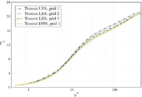
The quality of the LES simulations can be judged based on the comparison with the DNS results which are considered to be an exact solution of the Navier-Stokes equations. A quality index is introduced in Ref. [30] which is based on the total turbulent kinetic energy from the DNS, DNS
k , and the resolved turbulent kinetic energy from the LES, res
k . The local turbulent kinetic energy in both cases has been computed as:
2 2 2 ' ' ' 1 2 k u v v (A-1)where the bar sign above the velocity fluctuations indicates time average. The overall turbulent kinetic energy has been computed as the integral of equation (A-1) over the entire computational domain. The quality index is then given by the following equation _ 1 DNS res DNS k k IQ LES k (A-2)
The closer the index is to unity, the higher the “quality” of the LES simulations is, as it is able to capture more of the turbulent kinetic energy. The values of IQ_LES for our simulations are shown in Table 7. Note that the quality of all these LES simulations is high, as the resolved turbulent kinetic energy is >94% of the kinetic energy computed in the DNS simulation. By comparison, the quality index in the simulations has values of the order of 95%.
Obviously, the index in Eq. (A-2) cannot be the only measure by which the quality of a LES simulation is judged. Detailed comparison of the velocity and turbulent stress
distributions to their DNS counterparts also has to be made, as shown in the main body of the paper.
Table 7. Quality index for the LES simulations
LES for Re 400 Grid 1 Grid 2 Grid 3
_ smooth
IQ LES 0.941 0.957 0.967
_ hemisphere
IQ LES 0.99 0.995 0.997
The solution verification methodology recommended by Ref [31] was applied to both the LES and DNS simulations. Three solutions gk were obtained for different grid resolutions, for k= vc, c, f, where k is defined as 'very coarse (k=vc)', 'coarse (k=c)' and 'fine (k=f)', as shown in Tables II and III of the main body of the paper. The ratio of the signed error in the solution from one mesh refinement to the next can be used as a means to characterize the solution convergence:
( ) / ( ) 1 1 1 ( 1 0) f c c vc R g g g g
if R then monotonic convergence else if R then monotonic divergence else if R then oscillatory divergence else R then oscillatory convergence
(A-3)
For the solution verification analysis, one integral and one field variable were chosen as figures of merit: i) the space- (x and z directions) and time-averaged centerline (y=h) streamwise velocity, and ii) the turbulent kinetic energy of the entire domain (integral quantity). The results are shown in Table 8. The solution exhibits monotonic convergence for all figures of merit.
Table 8. Convergence for LES and DNS cases
LES smooth DNS smooth LES hemispherical
R (Ucent+) R (k) R (Ucent+) R (k) R (Ucent+) R (k)