HAL Id: hal-02596687
https://hal.archives-ouvertes.fr/hal-02596687v2
Submitted on 22 Nov 2013HAL is a multi-disciplinary open access archive for the deposit and dissemination of sci-entific research documents, whether they are pub-lished or not. The documents may come from
L’archive ouverte pluridisciplinaire HAL, est destinée au dépôt et à la diffusion de documents scientifiques de niveau recherche, publiés ou non, émanant des établissements d’enseignement et de
Assimilation of spatial distributed water levels into a
shallow-water flood model. Part II: using a remote
sensing image of Mosel river
Renaud Hostache, Xijun Lai, Jerome Monnier, Christian Puech
To cite this version:
Renaud Hostache, Xijun Lai, Jerome Monnier, Christian Puech. Assimilation of spatial distributed water levels into a shallow-water flood model. Part II: using a remote sensing image of Mosel river. Journal of Hydrology, Elsevier, 2010, 390 (3-4), pp.257-268. �10.1016/j.jhydrol.2010.07.003�. �hal-02596687v2�
Assimilation of spatially distributed water
levels into a shallow-water flood model. Part
II: use of a remote sensing image of Mosel
river.
Renaud Hostache
aXijun Lai
cJ´erˆome Monnier
bChristian Puech
aa
UMR TETIS, Cemagref, 500 rue JF Breton, 34093 Montpellier Cedex 5, France
b
INP-Grenoble & INRIA, Lab. LJK, B.P. 53, 38041 Grenoble Cedex 9, France
c
State Key Laboratory of Lake Science and Environment, Nanjing Institute of Geography & Limnology, Chinese Academy of Sciences, Nanjing, 210008, P.R.
China
Abstract
With rapid flood extent mapping capabilities, Synthetic Aperture Radar (SAR) im-ages of river inundation prove to be very relevant to operational flood management. In this context, a recently developed method provides distributed water levels from SAR images. Furthermore, in view of improving numerical flood prediction, a vari-ational data assimilation method (4D-var) using such distributed water level has been developed in Part I of this study. This method combines an optimal sense remote sensing data (distributed water levels extracted from spatial images) and a 2D shallow water model. In the present article (Part II of the study), we also derive water levels with a ± 40 cm average vertical uncertainty from a RADARSAT-1
im-age of a Mosel River flood event (1997, France). Assimilated in a 2D shallow water hydraulic model using the 4D-var developed method, these SAR derived spatially distributed water levels prove to be capable of enhancing model calibration. Indeed, the assimilation process can identify optimal Manning friction coefficients, at least in the river channel. Moreover, used as a guide for sensitivity analysis, remote sens-ing water levels allow also identifysens-ing some areas in the floodplain and the channel where Manning friction coefficients are homogeneous. This allows basing the spatial segmentation of roughness coefficient on floodplain hydraulic functioning.
Key words: Hydraulic modelling, roughness parameters, satellite SAR images, Digital Elevation Model, variational data assimilation, hydraulic coherence.
1 Introduction
Over the last decades, important efforts have been set up to better understand and manage floods, which is one of the most important natural hazard in the world. To identify flood prone areas and to manage flood events, satellite images could be very useful. Especially because of their all weather image acquisition capability, Synthetic Aperture Radar (SAR) sensors are relevant tools for the spatial characterization of floods. In this context, radar images of floods are nowadays mostly used for instantaneous flood extent extraction. Nevertheless, as mentioned by [25], there is no doubt that earth observation images contain information that goes beyond simple flood extents. In this context, [23] shown that high spatial resolution (25 m) SAR spaceborne images allow the estimation of distributed water levels in floodplains with reasonable
∗ Corresponding author.
uncertainty by merging SAR derived flood extent limits with a high-resolution high-accuracy Digital Elevation Model (DEM).
Furthermore, hydraulic modelling is of paramount importance in most flood forecasting and management systems. Due to huge stakes in flood manage-ment, the reliability of these flood inundation models is of primary concern. To be reliable, hydraulic models have to be constrained by using various ob-served data sets. The model calibration consists in forcing the model to provide outputs as close as possible to observed data by searching optimal values of its parameters. Generally, the main parameters to be calibrated in a hydraulic model are the roughness parameters (Manning coefficients) since these are dif-ficult to determine a priori. In an operational context, a “hand” calibration is often done through trial tests with the use of point observations, such as recorded hydrographs at stream gauges. Nevertheless these data are often in-sufficient to make the calibration reliable [1] as no reference data is available in the regions in-between those point measurements and a “hand” calibration is not accurate. As a matter of fact, taking into account complementary ob-servations in an advanced calibration could make a better constraining of the model and in return a better reliability. Spatially distributed data of a flood event, e.g.: water levels, would certainly help to enhance calibration reliability, but are very difficult to gauge in the field, especially due to the risk of peo-ple being injured. A rather simpeo-ple alternative way to obtain such distributed data is satellite imagery. Recent studies, [24, 14] have shown that SAR de-rived water levels allow the identification of Manning friction coefficients of one dimensional hydraulic models with a GLUE approach [3]. Furthermore, the recent improvements of mathematical tools provide more and more effi-cient means to calibrate numerical models. The variational data assimilation
method based on the optimal control theory of partial differential equations (also called 4D-var method) offers a special powerful tool to fuse in an opti-mal sense measurements (observations) and the mathematical model. In river hydraulics, variational data assimilation methods have been used successfully for shallow water models, see e.g. [6, 2, 22, 4,10, 7, 11,17, 12].
The present study aims at investigating whether the variational assimilation of water levels derived from a flood SAR image could help to enhance the calibration of flood inundation models. This would help getting benefits of both variational assimilation and recently developed remote sensing methods, improving flood model calibration.
Based on the study of [21], which provides water levels having an average un-certainty of ± 18 cm by using aerial photographs, the water level estimation method employed here is composed of three main steps [15]: i) extraction of the flood extent limits that are relevant to water level estimation, ii) primary estimation of water levels by merging the relevant limits and a high-resolution and high-accuracy Digital Elevation Model (DEM), iii) minimization of water level estimation uncertainties by hydraulic coherence constraints. This method is preferred in this study to the one developed by [23] since it can evaluate the observation uncertainty and does not need a one dimensional flow hypothesis. Regarding the variational data assimilation, we apply the method detailled to Part I, see [16].
The paper is organized as follows.
ground recorded hydrometric and remote sensing data. In Section 3, we present the methodology used to derive spatially distributed water levels from a SAR image. In Section 4, we recall very briefly the full mathematical and numeri-cal model, including the variational data assimilation process. In Section 5, we show the interest of assimilating SAR derived water levels in order to calibrate the Manning coefficients. This is done in two steps. First, we perform a twin experiment (i.e. observations are generated from direct model). This aims at evaluating the a priori potential efficiency of the assimilation process. Sec-ond, the identification of the hydraulic model friction parameters (Manning coefficients) is addressed by assimilating in situ and SAR derived observation. This is done by using various (and classical) land use based spatial distri-butions of the Manning coefficients. In Section 6, we perform the sensitivity analysis tests in order to evaluate if such a priori land-use based spatial distri-butions of the friction parameters leads to the most accurate numerical model.
2 Flood description and data extraction.
2.1 Study area
The area of interest includes a 28 km reach of the Mosel River between Uckange (France) and Perl (Germany) - see Fig. 1. In this area, the Mosel River me-anders in a flat plain having an average width of 3 km and a mean slope of 0.05 %. Most of the villages in the plain are located at an elevation slightly higher than the area covered by the February 1997 flood event. It is worth noting the presence of a narrow valley between Berg/Mosel and Perl cities
(Fig. 1). The latter behave as a bottleneck during flood events causing up-stream water retention area. In Perl city (downup-stream boundary), the Mosel basin has a size around 35500 km2
. The propagation velocity of the flood peak in the study area is low, around 2 km.h−1. The peak discharge recorded
at Uckange city stream gauge (upstream boundary) was around 1450 m3
s−1
(see Fig. 2), corresponding to a 4-5 year time return period [5]. Because of its representativeness of river inundations in floodplains, this area has already been investigated within the framework of the NOAH European project [18] and the PACTES French project [19] which aimed at analyzing the potential of remote sensing data - especially SPOT HRV images - for hydrological and hydraulic flood modelling. This shows the interest in analyzing this kind of river for generalizable methods.
2.2 Ground recorded hydrometric data
As hydrometric data, discharge hydrographs were available at three stream gauges located in the study area (see Fig. 1). These hydrographs are shown in Fig. 2. These have been provided respectively by the Environment Man-agement Direction of Lorraine (DIREN Lorraine), the French Company for Electricity (EDF) and the German Water Management and Navigation Di-rection (Wasser und Schifarts Direktion S¨udWest). The discharge hydrograph recorded in Perl hydrometric station looks contradict those recorded in EDF and Uckange hydrometric stations (no mass balance of water in the Mosel River during this flood event). Indeed, the water volume and the peak dis-charge recorded at Perl (downstream gauge station) during the flood events are higher (around 10 %) than those recorded in Uckange (upstream) and
EDF gauge stations (middle), although there is no lateral inflow in the study area and the variation of the basin area is negligible. As a matter of fact, these recordings are in opposition to the hydraulic principles of mass con-servation and peak discharge attenuation without inflow. Recorded discharge hydrographs araise from calculation using observed water stage hydrographs and rating curves: relationship between discharge and water level computed using discharge in situ measurements. Considering that higher magnitude dis-charges have been in situ measured in Uckange than in Perl for the the rating curve computation, the Uckange hydrograph has been assumed more reliable. As a consequence, only the discharge hydrographs in Uckange and EDF stream gauges are used as ground truth information in this study.
Consequently, available ground observations are fairly limited. The time series data of discharges at the EDF gauge station are only available at the begin-ning and the end of the flood period; the measurements are lacking during the high flood stage because of sensor disability (see Fig. 3).
2.3 Remote sensing data
The image used in this study has been acquired at 6:00 AM, during the Febru-ary 28th 1997 flood event, by the Synthetic Aperture Radar (SAR) sensor of the RADARSAT-1 satellite (descending orbit, standard beam S2, 5.6 cm wave-length, C band, Horizontal-Horizontal polarization). On C band radar images, the flood extent delineation is rather straightforward because the backscatter of smooth open water is very low due to specular reflection. However, wind may induce wavelets on water surface that may roughen it and increase its
backscatter. This may occur for the SAR sensor of RADARSAT-1 especially if these wavelets have vertical dimensions higher than 2.8 cm, according to Rayleigh’s criterion for a 5.6 cm C Band [26]. At the image acquisition time, the wind speed was moderate (7 m.s−1 in Metz city airport, French
Meteoro-logical Center record), thus the wind effects on open water surface roughness have been assumed negligible with respect to flooded area detection.
The SAR image, amplitude coded, has a pixel spacing of 12.5 m, resulting from the sampling of a complex image of 25 m spatial resolution. It was acquired a few hours after the flow peak, at the beginning of the recession, as shown in Fig. 2.
Furthermore, five air photographs at 1:15 000 scale, flown by the French Na-tional Institute of Geography (IGN) in 1999 out of flooding period, have been acquired. They have been used to digitize land use information : buildings, urban areas and sparse habitat, and high vegetation, forests, sparse trees, hedges etc. Indeed trees and buidings perturb the backscattering signal, so we choiced to mask these areas before processing : the whole process runs using only reliable areas.
The topographic and bathymetric raw data have been provided respectively by the North- Eastern French Navigation Services (SNNE) and the DIREN Lorraine as 3D points and 3D lines - calculated by photogrammetry using air photographs at 1:8 000 scale and SONAR sounding. The average altimetric uncertainty on the raw data is about 25 cm (DIREN information) for the floodplain and 1 cm (SNNE information) for the channel. Using a linear in-terpolation between points and lines, a Triangular Irregular Network (TIN)
Digital Elevation Model (DEM) has been generated and then converted to a RASTER DEM, easily superimposable with image data [13]. Hereafter, DEM acronym will be assigned to the topographic RASTER data. These interpola-tion choices are sufficient here, because main errors are not in the interpolainterpola-tion process : indeed, the initial data set (xyz points) is very dense, and sufficient to derive a good raster by linear interpolation ; moreover steep banks, poten-tially badly represented, are eliminated from the final process.
3 Water level estimation using SAR image
Based on the method developed by [21] providing water level estimates with a ± 18 cm mean uncertainty using flood aerial photographs, the water level estimation method used in this study is detailed in [15]. The current section presents the main steps and the general philosophy of this method. Using the RADARSAT image, this approach provides spatially distributed water level estimates within a ± 40 cm mean uncertainty. It can seem strange to reach such accuracy with large pixels (25m). Nevertheless, more than to pixel size, the accuracy in this process relates to DTM accuracy and the fact that the vertical estimates concern only places with very low slopes and no perturbing items (trees, houses ..).
3.1 Flood extent extraction
Flood extent mapping using SAR images is now a quite common issue [25] because water appears with very low backscatter compared to other objects.
In this study, to discriminate water from no-water on SAR images, radiomet-ric thresholding has been used because it is a robust and reliable way [9]. [15] shown that the use of a unique threshold value does not allow a satisfy-ing flood extent extraction since flooded areas may sometimes have the same backscattering values as non-flooded one in a SAR image. To deal with this radiometric uncertainty, the discrimination of flooded and non-flooded pixels is done using two threshold values. The first threshold value, Tmin, aims at
de-tecting only pixels that correspond to water bodies. Tmin has been determined
as the minimum radiometric value of non-flooded pixels inside grassland ar-eas (outside the floodplain and outside the permanent water surfaces) [15]. The second threshold value, Tmax, aims at detecting all flooded areas, at the
risk of detecting in addition non-flooded areas that have a similar radiometric value to the flooded one. Tmax has been determined as the maximum
radio-metric value of water bodies outside the flooded area, using the SAR image pixels located inside the Mirgenbach lake (see Fig. 1). The thresholding of the SAR image using Tmin and Tmax provide a flood extent map with fuzzy limits,
coded as follows (see [15]), depending on the intensity I of the SAR image pixels: 0 = non-flooded (I > Tmax), 1 = flooded (I < Tmin), 2 = fuzzy limit
(≈ potentially flooded) (Tmin ≤ I ≤ Tmax).
The innovative point of the SAR image processing is the analysis of the rele-vance of the remote sensing-derived flood extent limits for hydraulic purpose, and especially for water level estimation. To estimate water levels, the flood extent limits are merged with the underlying DEM. Using such a merging, any erroneous flood extent limit will lead to errors in water level estimation. Consequently, flood extent limits prone to error have to be identified before the merging. Errors in the flood extent limits are mainly due to emerging
objects such as building and high vegetation [15] that may mask water. To treat this potential errors, it has been chosen to remove all SAR derived flood extent limits located in habitat or vegetation areas. The remaining limits will be called relevant limits hereafter. Furthermore, since the flood extent limits are SAR image derived, they are prone to uncertainties arising mainly from the image spatial resolution and its georeferencing precision. To take account of these spatial uncertainties, the relevant limits have been enlarged (on both sides) using a distance equal to the sum of the image spatial resolution (25 m for the RADARSAT image) and the precision of the georeferencing (10 m for the RADARSAT image), as proposed in [15]. Considering that errors have been removed and that radiometric and spatial uncertainties have been taken into account previously, these “enlarged” relevant limits are then assumed to include the real flood extent limits (Hyp. 1 ). These are shaped as small patches which are sparsely distributed along the floodplain (Fig. 4).
3.2 Preliminary water level estimation
The second part of the process estimates one range of possible water levels IW LE = [W Lmin; W Lmax] for each relevant patch. To do so, the maximum
and the minimum elevation values are first extracted inside each relevant patch using the DEM Z values. Next, the DEM altimetric uncertainty (uncertDEM)
is taken into account by being respectively added/subtracted to the maxi-mum/minimum values extracted previously for each relevant patch:
IW LE = [min (Zpatch) − uncertDEM; max (Zpatch) + uncertDEM].
Since the DEM altimetric uncertainty is taken into account, Hyp. 1 allows to assume that each range of water level estimation - IW LE - includes the real
water level (Hyp. 2 ).
3.3 Final water level estimation
The last part of the process uses hydraulic rules to constrain the water level estimates and reduce their uncertainty, as proposed firstly by [20, 21]. In a floodplain, hydraulic laws manage the flow, so that water levels must follow an hydraulic logic : hydraulic energy decreases from upstream to downstream. With low flow velocity, like in the Mosel floodplain, this hydraulic rule can be simplified into a decrease of water level in the flow direction (Hyp. 3 ). To apply Hyp. 3 on the IW LE intervals, flow directions between patches (loca-tions of the water levels) have to be determined. As proposed in [15], some flow directions between patches have been determined using the shape of the SAR derived flood extent and the lines perpendicular to the elevation contour lines, oriented from the highest to the lowest elevation, called steeper lines hereafter. As a matter of fact, the knowledge of a up-/downstream relation-ship between two patches is conditioned by the connectivity of those on the SAR derived flood extent. If no hole in the flood extent is present between these two patches, an up-/downstream relationship can be determine. Fur-thermore, since the image has been acquired at the beginning of the flood recession, the main flow directions are assumed to be convergent toward the river channel, following the steeper lines. The steeper lines around relevant patches have been determined using the contour lines derived from the DEM. As a matter of fact, the sense of an up-/downstream relationship is given by the orientation of the steeper line. Using this criterion, some up/-downstream
relationship between patches have been determined. At the floodplain scale, these relationships constitute an hydraulic hierarchy of the relevant patches. Consequently, according to Hyp. 3, the water level must decrease from the patch A to the patch B if A is upstream of B. Due to Hyp. 2 this induce the following constraints:
Nmax(B) ≤ Nmax(A) (constraint on the maxima),
Nmin(A) ≥ Nmin(B) (constraint on the minima).
To apply these constraints, the algorithm that has been developed, is flow oriented and impose a decrease on the maxima from upstream to down-stream, and vice et versa, an increase on the minima from downstream to upstream. This finally provides intervals of constrained water level estimation IW LE = [W Lmin; W Lmax], with a half mean range of about ± 40 cm.
As a consequence, the method allow the definition of a set of distributed water levels across the floodplain at the satellite overpass time. These remote sensing-derived water levels are then used as new observation for the hydraulic modelling.
As a matter of fact, remote sensing derived data are assumed to be an obser-vation of water depth along the floodplain. The single image is extracted from the satellite image at 6:00 AM,Feb 28th,1997; The locations where the water level values have been extracted are shown in Fig.4.
4 Mathematical model with variational data assimilation (4D-var)
This section describes briefly the mathematical model with the variational data assimilation (4D-var) method. For more details, we refer to Part I of
the present study, [16], where the method has been validated on a test case. Numerical computations are performed by using the DassFlow software [10].
4.1 Mathematical model
The flood flow is modeled by the two-dimensional shallow water equations (2D-SWEs): ∂U ∂t + ∂F(U) ∂x + ∂G(U) ∂y = B(U) (1)
where x,y are the coordinates and t is the time, U is the state vector, F and G are the x- and y-directional flux vector respectively, B is the source term vector. These vectors are defined as follows:
U = (h, hu, hv)T = (h, qx, qy)T (2) F = (hu, hu2 + 1 2gh 2 , huv)T (3) G = (hv, huv, hv2 + 1 2gh 2 )T (4) B = (0, gh(S0x− Sf x), gh(S0y− Sf y))T (5)
where h is the water depth; u and v are the x- and y-directional velocity components; qx = hu and qy = hv are the unit discharge in the x- and
y-directions. S0x and Sf x are the bed and friction slopes, respectively along the
x axis and similarly S0y and Sf yfor the y axis. The friction slopes are evaluated
using the Manning formula.
The full inverse model (with variational data assimilation) includes the forward model (2D SWEs), the adjoint model and the minimization algorithm. The 2D-SWEs is solved using a finite volume method on unstructured meshes. The adjoint model is directly derived from the source codes of forward model by automatic differention [8]. The cost function J that has to be minimized
is defined in detail later (see (6) in the next section). As a matter of fact, the optimization problem to be solved is: minpJ(p), where p is the control
variable. The latter can be the initial condition, the Manning coefficient and/or inflow discharge.
4.2 Preliminary forward run
As a preliminary study, the Manning coefficients are set to an a priori ”reason-able” constant value, and the available data at inflow and outflow boundaries are used to perform a run of the forward model. Next, the simulation results are compared with the available measurements, namely the water stage hydro-graph at the middle gauge station (EDF) and the SAR image derived water levels in the floodplain at the satellite passover time.
The computational domain includes the main channel and the floodplain from Uckange to Perl. It is meshed using triangles and quadrilaterals elements and contains 2340 cells and 2430 nodes. The simulation time window begins at 12:00, Feb.25, 1997 and ends at 12:00, Mar. 2, 1997.
Initial conditions are computed as the steady state with constant inflow dis-charge at start time. At upstream boundary, the observed disdis-charge hydro-graph is imposed; at downstream, observed water stage hydrohydro-graph is imposed. The computational time step is set to two seconds (this respects the stability condition of the numerical scheme). The Manning coefficients are set to 0.025 all over the computational domain (this value is classically used to model the
present flow).
The observed and computed water stage hydrographs in the middle gauge station (EDF) are plotted in Fig. 5. Table 1 presents some basic statistics of the differences between the computed and the measured water levels in the floodplain (extracted from the image).
The computed water level at EDF gauge station (Fig. 5) is very close to measurements; while in floodplain at image time, the computed water level fits much less with available data, see Table 1. Thus, this preliminary forward run shows that the numerical model can reproduce the flow; and the current solution will be in next section an acceptable hand made first guess.
4.3 Cost function
As described in Part I of the present study, [16], the cost function J to be minimized (see section 4.1) contains three terms:
Jobs(p) = Jobs + αJf lux+ βJreg (6)
In (6) α and β are weight coefficients to be set and :
(1) Jobs corresponds to the discrepancy between the observations and the
computed flow state,
(2) Jf lux corresponds to the discrepancy of net mass flux,
(3) Jreg is a regularization term for smoothing time-dependent control
The weight coefficients α, β are setted by hand ”at best” in order to equili-brate the three terms after convergence. The cost function J depends on the control variable p since the state variable U depends on p.
The term Jf lux computes a ”mix” net mass flux since it is based on the
ob-served elevation hobs and the computed velocity (u, v)T, see Part I [16]. This
term enhances significantly the assimilation of the spatial distributed obser-vations in the floodplain (see Part I).
The term (Jobs + αJf lux) is defined as follows:
Jobs+ αJf lux= 1 2σ2 z ! m " zTimag(xm, ym) − z obs Timag(xm, ym) #2 [1 + α&(u, v)(xm, ym)& 2 ] + γ1 2σ2 Q [ $ T1 0 % Q(t) − Qobs(t)&2dt + $ T T −T2 % Q(t) − Qobs(t)&2dt] (7)
where σz and σQ are the standard deviations of observations, Timag is the
im-age time, (xm, ym) is the position of water level measurements, γ1 is a
weight-ing coefficient, T1 and T2 are the time periods of the discharge measurement
available at EDF station (see Fig. 3), T is the assimilation time period. The regularization term is:
Jreg(p) = 1 2 ' ' ' ' ' ∂Qin ∂t ' ' ' ' ' 2 (8)
5 Calibration of spatially distributed Manning friction coefficients (land-cover based spatial distribution)
The Manning friction coefficients n, that represents the resistance to the flow in channels and floodplains, are empirical and most of the time cannot be measured directly. It can be locally very fluctuant due to vegetation growing
or erosion deposition. In fact we must point out that (n) does not really exists, since it is strongly scale dependent, because it integrates all the friction pro-cesses at all scale. This section aims at showing the capability of SAR derived spatially distributed water levels to enhance the Manning coefficient calibra-tion, in comparison to a ”hand” calibration using trial-error tests. Thus, the data assimilation method presented here uses “orthogonal data”: water heights derived from water limits versus classical water depths in gauge station, see Fig. 3.
In this section, the spatial distribution of Manning friction coefficient is based on land-cover classes as classically done. Various cases have been considered depending on the total number of classes taken into account (between 1 and 10).
In the first approach, in order to investigate the reliability of our variational data assimilation process, while being free of measurement errors, twin exper-iments are performed: ”observations” are first generated using the numerical model (Manning coefficient being set a priori) and our variational data as-similation process is next used to retrieve the Manning coefficients used to generate the observed data.
In the second approach, the data assimilation is performed with the real ob-served data described in Section 2.
In all numerical experiments, the assimilation period is 66h from 12:00, Feb 25th (flood event starting time) to 6:00 AM, Feb 28th,1997 (SAR image ac-quisition time).
From a mathematical point of view the deal is different : here we want to verify that the method is able to retreive hidden values. Within the set of parameters, when (n) is the hidden value the method permits to retreive the initial value, which is in this case unique and well defined.
Land-cover classification
The domain is decomposed by using land-cover classes, one Manning coeffi-cient value n being set by land-cover class. Four various decompositions have been investigated, depending on the total class number:
a) a lumped n value: one constant value all over the domain.
b) three classes (distributed n) consisting of the main channel and the left and right floodplains (left and right banks present few differences in landuse. We are expecting close n values within banks, and strong differences with n main channel value).
c) five classes consisting of the main channel, the bridges (same n value for all bridges), the small lakes, and the left and right floodplains.
d) ten classes according to the land-cover classification presented in Fig. 6: main channel, bridges, small lakes, the left and right floodplains, vegetation, gravel, grassland, urban areas, downstream of the main channel.
5.1 Identification of Manning coefficients using synthetic data (twin experi-ments)
The identification process in the first approach is based on synthetic data. This means that given some Manning coefficients values, observations are generated by running the model. Then, the aim is to retrieve these Manning coefficients
which are used to generate observations. Such experiments are called as twin experiments. They can test the reliability of the identification process, while being free of measurement errors, and then to evaluate the potential efficiency of the variational data assimilation process for identifying correctly the Man-ning coefficients.
It is worth noting that the synthetic data are generated exactly at the same locations as those of the real observations. The difference is that they is gen-erated by the exact forward model.
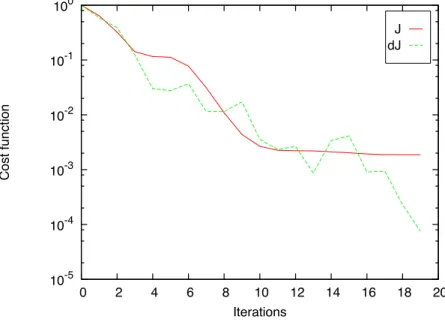
For the sake of clarity, we consider here case b) only (see above) i.e. three land-cover classes. Fig. 7 shows the decreases of the normal cost function and its normal gradient vs iterations (convergence of the optimization process).
Table 2 presents the results obtained when considering three land-cover classes (case b). We start from one initial guess value (i.e. a single value for the three classes), and we compute the three optimal values corresponding to the three classes. Table 2 shows that the variational data assimilation process is capable of retrieving the three initial Manning coefficient values (”true” values): in the main channel, in the right and left floodplains.
Let us point out that various numerical experiments have been performed to corroborate this result. Indeed, we started the optimization process with var-ious initial guesses (e.g. n0 = 0.020, 0.033 , 0.050), and all of them converged
to the same optimal values, equal to the guesses.
The present identification experiment based on synthetic data, shows that the SAR derived spatially distributed water levels and the stream gauge in-situ measurements can identify properly the spatial distributed Manning coeffi-cients, at least if three land-cover classes only are considered and if the
math-ematical model is perfect (i.e. observations corresponds to the modelled flow) and no error is introduced in measurements. These last two features are very important. In next section, we use the real data and we will notice that the (real) identification problem is much more difficult to solve numerically, even with three land-cover classes only.
5.2 Identification of Manning coefficients using real data
In the second approach, the same identification process as in the previous section has been performed, but under the real observations. The upstream and downstream boundary conditions are respectively the observed discharge hydrograph in Uckange and the observed water stage hydrograph in Perl (see section 2). The initial condition is calculated as a steady state simulation of the model, using as boundary conditions the discharge and the water level ob-served respectively in Uckange and Perl at the simulation starting time. Then, given initial guesses for Manning coefficient values (see n0 values in Table 3),
the optimal values, i.e. minimizing the cost function J, are sought. For each case (lumped n, three, five or ten land-cover classes), the same minimum value of J is obtained.
Table 3 presents the initial and optimal computed n values for each case (de-pending on the land-cover number). In all cases, the computed value of the main channel is the same whatever the initial guess n0(e.g. 0.033, 0.020, 0.025
or 0.050) and the total class number. On the contrary, n in other land-cover classes are almost not modified during the optimization process. This result is consistent with the forthcoming sensitivity analysis (see next section), runs which shows that the total cost function is almost insensitive to the n values
outside the main channel.
In twin experiments performed previously, data were perfect since they were created by the model. In that case, the cost function was much less insensitive to the two n values outside the main channel. That is why numerical identifi-cation was accurate and robust, Table 2.
Using real data, sensitivities can become different, and the identification prob-lems become much more difficult. In the present case, the few sensitivity of the model to the Manning coefficient outside the channel is mainly due to the rather low time return period of the investigated flood event (4-5 year). Indeed, for the 1997 flood event the most important part of the flow occurred in the channel. As a result, since the Manning equation is used to compute the friction slope, even a drastic change in the floodplain Manning coefficient value implies a low variation of water level when the discharge is low in the floodplain. This consideration shows that the water levels in the floodplain is more influenced by the water level inside the channel (and thus by the channel Manning coefficient) instead of the floodplain Manning coefficient.
In the case of a lumped n, we present in Table 1 some statistics on the differ-ence between the simulated and the SAR derived water levels (where image information is available). Compared to the results obtained with the prelim-inary forward run, the present results show a significant improvement since the error indicators are drastically lowered. In Fig. 8 and Fig. 9, we plot the difference between the computed and the observed water level where image information is available and when considering one, three and ten land-cover classes. Fig. 10 shows the comparison between simulated and observed dis-charge hydrographs at the EDF middle gauge station (in function of time).
These results show that after the identification of an ”optimal” set of Manning coefficient values, the computed flow state is much closer to the observations than that computed using the forward hand-calibrated model (i.e. with n val-ues resulting of many trial-error tests).
6 Sensitivity analysis and Manning decomposition
The previous section shows that our variational data assimilation process is capable of enhancing significantly the calibration of the distributed Manning friction coefficients, and consequently the accuracy of the numerical model. Nevertheless, all computations have been done with an a priori: the Manning coefficients have been defined spatially distributed according to given land-use classes (between 1 and 10). This a priori is rather traditional. Nevertheless, does this necessary lead to the most accurate numerical model ?
In the current section, we aim at answering to this question. To meet this aim, a sensitivity analysis is performed without any a priori for the Manning spatial distribution (i.e. any land-use is defined).
One run of the forward model plus the adjoint model, without running the full optimization process, gives the gradient of cost function J with respect to the Manning coefficients. These gradient values represent the local sensitivity of the cost function with respect to the Manning coefficients. They help one to understand which Manning area is the most important to calibrate.
The ten land-use case
First, we perform sensitivity analysis in the case the Manning is decomposed by the ten land-uses defined previously, see Fig. 6. We show the ten spatially distributed gradient values in Table 4 and Fig. 11.
These gradient values are computed for a constant Manning value over the whole domain (n = 0.033); sensitivity results are similar if computed from different Manning coefficient values (n = 0.05 or n = 0.01 for example).
This sensitivity analysis suggests that the most important Manning value to focus on is in the main channel, than much less important are the vegetation area, the bridge (in main channel), gravel area and grassland area. Others land-use values are negligible.
This sensitivity analysis result is consistent with the calibration process pre-sented in previous section: the optimization algorithm calibrate essentially the main channel value.
No a priori land-use case
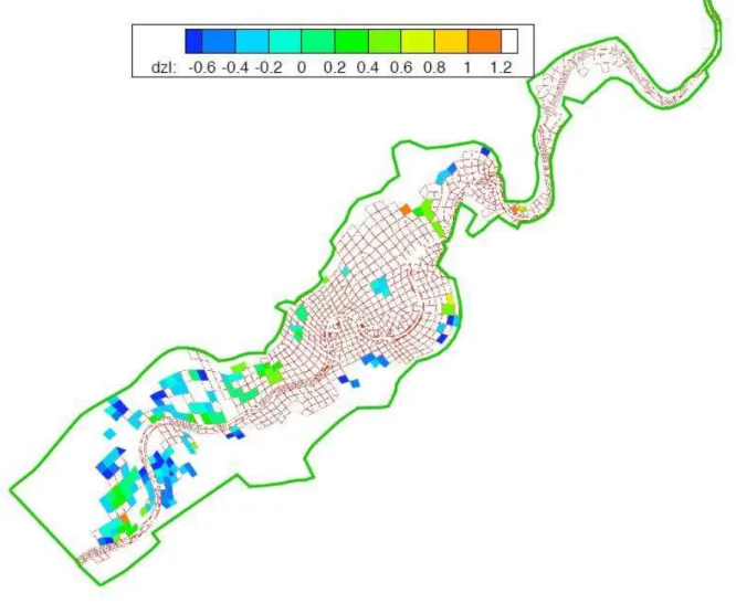
Next, a sensitivity analysis with no a priori on the Manning decomposition has been performed: we define one Manning value for each mesh cell, and we compute the gradient value for each cell. In particular in the main channel, there are as many potential values as cells. The computed spatially distributed gradient values are shown in Fig. 12.
main channel (at least four in the present case). More generally, this suggests to define the Manning areas not upon the land-use (or land-cover) but upon ”sensitive areas”. Furthermore, the combination of the satellite image and runs of sensitivity analysis indicate the most important Manning areas we need to calibrate (including inside the main channel).
7 Conclusions
Part I of this study [16], presents a method to assimilate spatially distributed water levels into a shallow water model. The present article (Part II) deals with an application of the assimilation method into a real test case, in order to in-vestigate the value of remote sensing-derived water levels for improving model reliability, variational methods are used in assimilation. By using a variational data assimilation approach (4D-var), we have investigated potential contribu-tions of SAR derived spatially distributed water levels for the identification of time-independent parameters (Manning coefficients) in a shallow-water flood model.
The spatially distributed water levels have been derived from a SAR image by employing the method developed in [15]. They have been obtained with a ± 40 cm mean uncertainty, using a RADARSAT-1 image of the 1997 flood event of the Mosel river. This has been possible by using both an analysis of the relevance of SAR derived flood extent limits for hydraulic purposes, and a merge between the relevant limits and a highly resolution DEM, under hydraulic coherence constraints inspired from [20, 21]. Such a water level es-timation provides spatially distributed information at the time of a satellite overpass while classical in situ measurements are punctually available.
Furthermore, numerical experiments conducted in this study indicate that a rather dense information in space is of great benefit for the identification of unknown parameters (Manning friction coefficient). Indeed, the assimilation of the SAR derived water levels, in addition to an incomplete discharge hy-drograph, proves to be capable of identifying Manning friction coefficients, while the ground data alone does not allow such an identification. Further-more, a sensitivity analysis conducted by using the SAR derived water levels, shows that a spatial distribution of the friction coefficient based on land-cover may not necessarily lead to the better model results. Indeed, these water lev-els, used as a guide in the sensitivity analysis, can define areas of Manning friction homogeneity, without apparent link with land-cover. Such sensitivity analysis may finally base the Manning parameter spatial distribution more on the model hydraulic functioning, than on the land-cover.
The most important issue in flood forecast is to predict the flood peak. We know that remote sensing images cannot be useful in predicting directly flood peaks except in regions with very slow flood events. Our process leads to a better model, more physically constrained, which helps to reduce equifinality, and can be used for future predictions.
This study contributes to the basic understanding of the assimilation of spa-tial distributed water levels into a shallow-water flood model. It demonstrates that the use of satellite images improves parameter identification capability and thus flood prediction. As a consequence, the study presents two main ad-vantages. It provides distributed water levels with a high spatial density over large areas and provides more reliable hydraulic models. In a near future, with the launch of new radar satellites (e.g. RADARSAT-2, ALOS, Cosmo-skymed, TerraSar-X) with better spatial and radiometric resolutions and more suitable wavelength, the uncertainties of water levels estimates will presumably be
fur-ther reduced. The capability of SAR derived water levels may be enhanced to help the identification of model parameters using variational assimilation.
Acknowledgment
This research has been supported by R´egion Rhˆone-Alpes, France ( ”numeri-cal prevention for floods” project 2003-2006).
The authors would like to acknowledge Andr´e Paquier (Cemagref Lyon, France) for his help in the definition of the preliminary forward run, Joel Marin (IN-RIA Rhˆone-Alpes) for his help in computational issues. The authors would like to thank the reviewers for their detailed comments that has helped to improve the paper.
English writing has been improved thanks to National Natural Science Foun-dation of China (Grant No. 50709034).
References
[1] G. Aronica, B. Hankin, and K. Beven. Uncertainty and equifinality in calibrating distributed roughness coefficients in a flood propagation model with limited data. Advances in Water Resources, 22:349–365, 1998. [2] E. Belanger and A. Vincent. Data assimilation (4D-VAR) to forecast
flood in shallow-waters with sediment erosion. Journal of Hydrology, 300:114–125, 2005.
[3] K. Beven and A. Binley. The future of distributed models - model cali-bration and uncertainty prediction. Hydrological Processes, 6(3):279–298, 1992.
[4] W. Castaings, D. Dartus, M. Honnorat, F-.X. Le Dimet, Y. Loukili, and J. Monnier. Automatic differenciation: a tool for variational data assim-ilation and adjoint sensitivity analysis for flood modeling. Lecture Notes in Computational Science and Engineering, 50:249–262, 2006.
[5] Minist`ere de l’´Ecologie et du D´eveloppement Durable. Banque hy-dro : Banque nationale de donn´ees pour l’hyhy-drologie et l’hyhy-drom´etrie, http://www.hydro.eaufrance.fr/.
[6] Y. Ding, Y. Jia, and S.Y. Wang. Identification of Manning’s roughness coefficients in shallow water flows. Journal of Hydraulic Engineering, 130(6):501–510, 2004.
[7] I. Gejadze and J. Monnier. On a 2d zoom for 1d shallow-water model: coupling and data assimilation. Comp. Meth. Appl. Mech. Eng., 196(45-48):4628–4643, 2007.
[8] L. Hascoet and V. Pascual. Tapenade 2.1 user’s guide. Technical Report RT–300, INRIA, project Tropics, www-sop.inria.fr/tropics, 2004.
[9] J.-B. Henry. Syst`emes d’information spatiaux pour la gestion du risque d’inondation de plaine. PhD thesis, Universit´e de Strasbourg I, 2004. [10] M. Honnorat, J. Marin, J. Monnier, and X. Lai. Dassflow v1.0: a
varia-tional data assimilation software for river flows. Research report INRIA RR-6150, 2007.
[11] M. Honnorat, J. Monnier, and FX. Le Dimet. Lagrangian data assimi-lation for river hydraulics simuassimi-lations. Comput. Visual. Sc., 12(3):235, 2009.
[12] M. Honnorat, J. Monnier, N. Rivi`ere, E. Huot, and FX. Le Dimet. Identi-fication of equivalent topography in an open channel flow using lagrangian data assimilation. Comput. Visual. Sc., 13(3):111, 2010.
car-act´erisation tridimensionnelle de l’al´ea et l’aide `a la mod´elisation hy-draulique. PhD thesis, ENGREF, 2006.
[14] R. Hostache, P. Matgen, G. Schumann, C. Puech, L. Hoffmann, and Pfis-ter L. WaPfis-ter level estimation and reduction of hydraulic model calibration uncertainties using satellite sar images of floods. IEEE Transactions on Geoscience and Remote Sensing, 47(2):431–441, 2009.
[15] R. Hostache, C. Puech, G. Schumann, and P. Matgen. Estimation de niveaux d’eau en plaine inond´ee `a partir d’images satellites radar et de donn´ees topographiques fines. Revue T´el´ed´etection, 6(4):325–343, 2006. [16] X. Lai and J. Monnier. Assimilation of spatial distributed water levels
into a shallow-water flood model. part i: mathematical method and test case. J. Hydrology, 377(1-2):1–11, 2009.
[17] J. Marin and J. Monnier. Superposition of local zoom model and simul-taneous calibration for 1d-2d shallow-water flows. Math. Comput. Simul., 80:547–560, 2009.
[18] NOAH. New oportunities of altimetry in hydrology, final report. Techni-cal report, Cemagref, BFG, Delf Hydraulics, 2000.
[19] C. Puech, G. Galea, and J.B. Faure. Flood forecasting and prevention using remote sensing data (PACTES) final report of cemagref contribu-tion. Technical report, Cemagref, 2002.
[20] C. Puech and D. Raclot. Using geographical information system and aerial photographs to determine water levels during floods. Hydrological processes, 16(8):1593–1602, 2002.
[21] D. Raclot. Remote sensing of water levels on floodplains: a spatial ap-proach guided by hydraulic functioning. International Journal of Remote Sensing, 27(12):2553–2574, June 2006.
techniques in open-channel inverse problems. J. Hydraul. Res., 43:311– 320, 2005.
[23] G. Schumann, R. Hostache, C. Puech, L. Hoffmann, P. Matgen, F. Pap-penberger, and L. Pfister. High-resolution 3D flood information from radar imagery for flood hazard management. IEEE Transactions on Geo-science and Remote Sensing, 45(6):1715–1725, 2007.
[24] G. Schumann, L. Matgen, L. Hoffmann, R. Hostache, F. Pappenberger, and L. Pfister. Deriving distributed roughness values from satellite radar data for flood inundation modelling. Journal of Hydrology, 344:96–111, 2007.
[25] L.C. Smith. Satellite remote sensing of river inundation area, stageand discharge: A review. Hydrological Processes, 11(10):1427–1439, 1997. [26] F.T. Ulaby and M.C. Dobson. Handbook of radar scattering statistics for
List of Tables
1 Difference between the computed and the measured water
depth (m) in floodplain (data extracted from the image). 34
2 Twin experiments. Identified Manning coefficients n. Example based on three land-cover classes: case b). 34
3 Real data. Identification of Manning coefficients. Initial guesses n0 and identifed values n for each cases (i.e. optimal values
computed). 35
4 Sensitivity analysis. Gradient values for case d) 10 land-uses
(at Manning value constant everywhere n = 0.033) 36
List of Figures
1 Study area of the Mosel River and RADARSAT image 37
2 Recorded hydrographs during the flood event at 3 different
locations 38
3 Observations available: discharge at low water level at EDF
gauge station and one (partial) image 39
4 Spatial distribution of water level values available after image
5 Preliminary forward run. Comparison of discharge (m3
/s) at the middle gauge station EDF: measured, computed with elevation imposed at downstream (”Z”), computed with water stage hydrograph imposed at downstream (”QZ-org”). 41
6 Land cover: 10 classes (Case d) in the text). 42
7 Convergence of the minimization process. Plotted: the normal cost function J (solid line), the normal gradient dJ (dashed line). Case considered: Manning calibration with synthetic
data for 3 classes (case b). 43
8 Water levels (m) at image blocks i.e. where image information is available (see Fig. 4). Vertical bars corresponds to the measures with estimated uncertainties. The four curves corresponds to the preliminary forward run and the three calibrated models responses (depending on the land classes number considered; VDA-nXX = 1, 3 and 10 land classes). (Recall: VDA=Variational Data Assimilation = 4D-VAR
algorithm; direct = forward model without calibration.) 44
9 Difference of water depth (m) at image instant (6:00, Feb 28th, 1997) between observations and computed values using the calibrated model (Manning is calibrated in 3 land classes,
10 Measured discharge hydrographs (m3
/s) at the middle gauge station EDF, and computed ones using the calibrated model (Manning is calibrated in 3 land classes, case b)). ”Z”: computed values with elevation imposed at downstream; ”QZ-org”: computed values with water stage hydrograph
imposed at downstream. 46
11 Sensitivity analysis. Gradient value: cost function with respect to the Manning coefficient if 10 land blocks are considered
(case d). 47
12 Sensitivity analysis. Gradient value: cost function with respect to the Manning coefficient in each finite volume cell (no
Table 1
Difference between the computed and the measured water depth (m) in floodplain (data extracted from the image).
Max Mean Min Standard Deviation ( (h − hobs)2
Preliminary forward run 2.297 0.466 -0.389 0.406 54.175
Real data, case a) 1.239 0.036 -0.869 0.283 11.628
(one lumped value) Table 2
Twin experiments. Identified Manning coefficients n. Example based on three land-cover classes: case b).
Land class True n Land use Computed n
1 0.025 Main channel 0.0251
2 0.04 Right floodplain 0.0406
Table 3
Real data. Identification of Manning coefficients. Initial guesses n0 and identifed
values n for each cases (i.e. optimal values computed).
case a) case b) case c) case d)
Lumped n Three classes Five classes Ten classes
n0 n n0 n n0 n n0 n 1 0.025 0.0146 0.020 0.0153 0.050 0.0151 0.033 0.0156 2 0.020 0.0199 0.050 0.0497 0.05 0.0499 3 0.020 0.0198 0.050 0.0489 0.033 0.0324 4 0.050 0.0495 0.033 0.033 5 0.050 0.0498 0.033 0.033 6 0.033 0.033 7 0.033 0.0322 8 0.033 0.0328 9 0.033 0.033 10 0.100 0.100
Table 4
Sensitivity analysis. Gradient values for case d) 10 land-uses (at Manning value constant everywhere n = 0.033)
Channel Vegetation Bridge Gravel Grassland
881.54 e+6 43.75 e+6 17.76 e+6 3.64 e+6 -1.06 e+6
Left Right Snaked land Urban Downstream channel
Flo
w
dire
cti
on
Uckange
stream gauge
(Upstream)
Berg/Mosel
Village
To
wa
rd
Pe
rl
Perl
stream gauge
(Downstream)
EDF
stream gauge
(Middle)
Mosel channel
Flooded
area
Lake
Meters25feb1997 12000 27feb1997 1200 01mar1997 1200 03mar1997 1200 200 400 600 800 1000 1200 1400 1600 Date Discharge [m 3 .s − 1 ] Uckange (Upstream) EDF (Middle) Perl (Downstream) SAR Image
0 200 400 600 800 1000 1200 1400 0 20 40 60 80 100 120 discharge (m 3 /s) time (h) T1 T2
Image time (Timag) Unavailable
Avail. data
Fig. 3. Observations available: discharge at low water level at EDF gauge station and one (partial) image
Unavailable water level values Available water level values River channel
0 200 400 600 800 1000 1200 1400 0 20 40 60 80 100 120 d is c h a rg e (m 3 /s) time (h) EDF hydrograph Measured Z QZ-org
Fig. 5. Preliminary forward run. Comparison of discharge (m3
/s) at the middle gauge station EDF: measured, computed with elevation imposed at downstream (”Z”), computed with water stage hydrograph imposed at downstream (”QZ-org”).
10-5 10-4 10-3 10-2 10-1 100 0 2 4 6 8 10 12 14 16 18 20 Cost function Iterations J dJ
Fig. 7. Convergence of the minimization process. Plotted: the normal cost func-tion J (solid line), the normal gradient dJ (dashed line). Case considered: Manning calibration with synthetic data for 3 classes (case b).
Fig. 8. Water levels (m) at image blocks i.e. where image information is available (see Fig. 4). Vertical bars corresponds to the measures with estimated uncertainties. The four curves corresponds to the preliminary forward run and the three calibrated models responses (depending on the land classes number considered; VDA-nXX = 1, 3 and 10 land classes). (Recall: VDA=Variational Data Assimilation = 4D-VAR algorithm; direct = forward model without calibration.)
Fig. 9. Difference of water depth (m) at image instant (6:00, Feb 28th, 1997) between observations and computed values using the calibrated model (Manning is calibrated in 3 land classes, case b)).
Fig. 10. Measured discharge hydrographs (m3
/s) at the middle gauge station EDF, and computed ones using the calibrated model (Manning is calibrated in 3 land classes, case b)). ”Z”: computed values with elevation imposed at downstream; ”QZ-org”: computed values with water stage hydrograph imposed at downstream.
Fig. 11. Sensitivity analysis. Gradient value: cost function with respect to the Man-ning coefficient if 10 land blocks are considered (case d).
Fig. 12. Sensitivity analysis. Gradient value: cost function with respect to the Man-ning coefficient in each finite volume cell (no a-priori land block is done).