Flow Architectures for Ground-Coupled Heat Pumps

HAL Id: hal-01847550

https://hal.insa-toulouse.fr/hal-01847550

Submitted on 4 Mar 2019

HAL is a multi-disciplinary open access

archive for the deposit and dissemination of

sci-entific research documents, whether they are

pub-lished or not. The documents may come from

teaching and research institutions in France or

abroad, or from public or private research centers.

L’archive ouverte pluridisciplinaire HAL, est

destinée au dépôt et à la diffusion de documents

scientifiques de niveau recherche, publiés ou non,

émanant des établissements d’enseignement et de

recherche français ou étrangers, des laboratoires

publics ou privés.

Flow Architectures for Ground-Coupled Heat Pumps

Sylvie Lorente, A. Bejan

To cite this version:

Sylvie Lorente, A. Bejan. Flow Architectures for Ground-Coupled Heat Pumps. ASME 2016

In-ternational Mechanical Engineering Congress and Exposition, Nov 2016, Phoenix, United States.

�10.1115/IMECE2016-65410�. �hal-01847550�

FLOW ARCHITECTURES FOR GROUND-COUPLED HEAT PUMPS

S. Lorente

University of Toulouse, INSA, LMDC, Toulouse, France

A. Bejan Duke University Durham, NC, USA

ABSTRACT

In this paper we report the main advances made by our research group on the heat transfer performance of complex stream architectures embedded in a conducting solid. The immediate application of this review work deals with ground-coupled heat pumps. Various configurations are considered: U-shaped with varying spacing between the parallel portions of the U, serpentines with three elbows, and trees with T- and Y-shaped bifurcations. In each case the volume ratio of fluid to soil is fixed. We determine the critical geometric features that allow the heat transfer density of the stream-solid configuration to be the highest that it can be. In the case of U-tubes and serpentines, the best spacing between parallel portions is discovered, whereas the vascular designs morph into bifurcations and angles of connection that provide progressively greater heat transfer rate per unit volume. Next we move to more complex underground structures, connecting several heat pumps to the same fluid loop. We conclude by comparing the merits of the two options.

Keywords: constructal, tree structure, vascular design, dendritic, ground heat pump.

INTRODUCTION

An important application of constructal design [1] is the enhancement of the thermal contact between a heat pump and the ground. There is growing interest in designs that improve the performance of ground coupled heat pump systems [2-9]. In this review paper we consider the fundamental configuration of

time-dependent heat transfer between the ground and U- T- and Y- shaped and serpentine pipes that function as heat sources or sinks. We then connect several heat pumps to a unique underground pipe loop. The design work described in this paper is the search for pipe-ground configurations that promise effective and compact heat transfer, and high thermodynamic performance for the heat pump system connected thermally to the ground. The fundamental aspect is the focus on the discovery of flow configuration: the relation between the morphing of the flow configuration and the improvements in the global performance of the complex flow system, in accord with constructal theory [10]. NOMENCLATURE D ₌ channel diameter, m H ₌ Height, m k ₌ thermal conductivity, Wm–1_K–1 L ₌ channel length, m

m = mass flow rate, kg s−1 n = number of bifurcation levels P = pressure, Pa

Pe = Peclet number Pr = Prandtl number Q = Enthalphy, J S = Spacing, m

Proceedings of the ASME 2016 International Mechanical Engineering Congress and Exposition IMECE2016 November 11-17, 2016, Phoenix, Arizona, USA

Sv ₌ Svelteness number T ₌ temperature, K t = time, s V = volume, m3

Vh = volume of heated solid, m3 W = Width, m x, y, z = coordinate, m Greek Symbols α = thermal diffusivity, m2 _s−1 β = bifurcation angle θ = dimensionless temperature  = Density, kg m-3

φ = composite volume fraction (porosity) Subscripts and superscripts

∞ = infinite

THEORETICAL FORMULATION

The pipe is buried in the ground (Fig. 1), which is modeled as a cube. We begin with the simplest shape, which is a pipe shaped as the letter U inside a cube [11]. The volume fraction , calculated as the ratio of the pipe volume Vfand the volume of soil V, can vary. The spacing between the parallel portions of the U-shaped pipe is S, and the pipe diameter is D. The outer surface of the cube is adiabatic. The cube volume is fixed, however, the shape of the volume can be changed. The total length of the pipe is L. The pipe slenderness ratio L/D is fixed. The ground is initially at a higher temperature (T∞) than the fluid in the pipe (Tp). A cooled zone grows around the pipe.

U configurations are considered with various S/D ratios. The conservation equations for mass and momentum in the fluid flow are solved by means of a finite elements package [12]. The ground is initially at a temperature T∞. The fluid enters the pipe at Tin. The dimensionless fluid temperature is defined as

in

T

T

T



T







  ₍₁₎ SERPENTINE IN A CUBE

Four different shapes are shown in Fig. 2. The U shape with S/D = 15 was chosen because the spacing between inlet and outlet is the same as three times the spacing between the turns of the serpentines, S/D = 5. The pipe volume length and diameter are fixed (L/D = 45), and the corresponding flow volume fraction represented by the pipe is φ = 0.002. The thermal performance of the pipe shapes is plotted in Fig. 3. The better shape is serpentine 2.

As time increases, the solid volume temperature approaches the fluid inlet temperature. As a measure of the time needed to approach equilibrium, we selected the non-dimensional time t_ss* whenθout reaches 80% of the equilibrium level, (θout = 1),

out ss

out t( *)0.8

 (2)

Figure 1 U-shaped pipe inside a cube when S/D = 5 [11].

Figure 2 Four pipe shapes in a solid cube [11]. avg = average

f = fluid in = inlet

Figure 3 The outlet temperature in the four configurations of Fig. 2 [11].

TREE-SHAPED FLOW CONFIGURATIONS WITH 90° ANGLES OF CONNECTION

An alternative is to replace the serpentine configuration with dendritic structures [13]. As shown in the lower part of Fig. 4, every channel of the tree is a round tube of diameter Diand length Li. The tree-shaped designs are configured as two palms facing each other. One tree spreads the fluid from the point (heat pump) to the ground area, and the other collects the fluid from the ground and returns it to the heat pump. We account for the entire fluid volume in our analysis (when discussing volume fraction).

The pipe diameters vary stepwise in accord with the Hess-Murray rule [1],

2 1/3 D

D_i_{1 i}   , laminar (3) The porosity, and the Svelteness number [13] are  = Vf/V and

3 / 1 n 1 i 2 i i 1 I n 1 i 1 3 / 1 f Total D L 4 2 L V L scale length flow external ernal int scale length flow external S             





   (4)

We simulated numerically the evolution of the flow and temperature field in four configurations (n = 1, ..., 4). The fluid flow is specified by the mass flow rate into to the trunk and the outlet pressure (P0= 0) at the extremities of the smallest pipes. The flow was in the laminar regime, because in every pipe the Reynolds number did not exceed the order of 103_{. Figure 5} shows that the approach to equilibrium is faster when the complexity increases. The approach to final equilibrium is faster when the number of branches is greater.

Next, we give the structure the freedom to morph [14]: The usual proposal that led to tree design in fluids and heat transfer engineering is to first assume a fixed tree architecture and next to determine its performance [1]. Here the tree architecture,

with all its angles and lengths, is the unknown. The tree structures are based on the search for the angles of bifurcation that lead to maximum heat transfer density. As an example, Fig. 6 shows the optimal angle β4 for maximum avg, and Fig. 7 shows the corresponding temperature field around the tree structure for every optimized angle.

Figure 4 Tree-shaped configurations [13].

Figure 5 The effect of complexity (n) on the evolution of the system average temperature in a three-dimensional configuration [13].

Figure 6 The optimization of bifurcation angle β4 when β1 = 101°, β2 = 81° and β3= 85° in a larger cube [14].

the buried ducts, which act as heat sink. In time, the volume averaged temperature of the cube decreases and approaches T∞. We are interested in the effect of each configuration on the approach to thermal equilibrium. For this purpose, we investigated the effect of tree and classical geometry on the average temperature of the cube at that time.

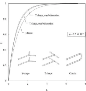
We compared the heat transfer performance of the evolutionary Y, T and classical design when the tree with the same number of bifurcation levels (N) and each design was constructed with same volume fraction φ . This was reviewed in [15]. Figure 8 shows theaveragedtemperatureθavg,whentheY andTshapes have one bifurcation level. The spacing between the planes of the palm-to-palm tree is equal to the length of the branch of the Y or T. The steeper curve represents the design with better thermal contact between architecture and conducting medium, and the better design is the evolutionary tree with Y-shaped bifurcation.

Figure 7 The temperature field around the tree in a large solid: (a) Trunk; (b) Tree when β1= 95°; (c) Tree when β1= 95° and β2 = 80° (β2A= β2B = 40°); (d) Tree when the optimization is repeated and β1= 100°, β2= 80° (β2A= β2B = 40°); (e) Tree when β1= 100°; β2= 80° (β2A= β2B= 40°) and β3= 85° (β3A= β3B= 42.5°); (f) Tree when the optimization is repeated and β1 = 101°, β2= 81° (β2A= β2B= 40.5°) and β3= 85° (β3A= β3B= 42.5°); (g) Tree when β1= 101°, β2 = 81° (β2A= β2B = 40.5°), β3 = 85° (β3A= β3B= 42.5°) and β4 = 70° (β4A = 40° β4B = 30°) and (h) Tree when the optimization is repeated and β1= 105°, β2= 82° (β2A= β2B= 41°), β3= 85° (β3A= β3B= 42.5°) and β4= 70° (β4A= 40° β4B = 30°) [14].

Figure 8 Thermal performance of Y-shaped, T-shaped and classical designs [14].

ONE UNDERGROUND HEAT EXCHANGER

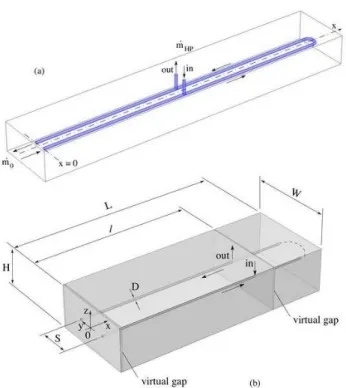
The objective of this section is to determine the configuration (the layout) of the heat exchanger and multiple heat pumps so that the performance of the whole assembly is increased. Several heat pumps operate with heat transfer to and from a single heat exchanger buried in the ground [16]. Assume that a heat pump is connected at x = 0 (Fig. 9a). There a baseline mass flow rate

m



₀ that comes from the pre-existing piping (from the left in Fig. 9), enters in one leg and returns along the other. The heat pump is connected such that the fluid intake is on one leg and the outflow is in the opposite location on the other leg. The heat pump position is at x = l, which varies as a design parameter. The pipes reside in the horizontal plane x-y with centers at y = S/2. The heat pump feeds the buried pipe with a mass flow rate of

m



_HP at a specified temperature Tin. The heat pump retrieves the flow rate

m



_HPat a higher temperature.

The ground volume (V = LWH) is shown in Fig. 9b. The heat transfer through the soil is modeled as steady-state heat conduction. We are interested in the design of the underground heat exchanger and in how to position the heat pumps along it. Therefore we assume that the connections between a heat pump and the U pipe can be modeled as sudden mixing.

Figure 9 (a) Long serpentine loop buried in a parallelepipedic volume of soil with one heat pump connected at the distance l from the mid plane. (b) Physical model considered for the numerical simulation with the virtual connection of the heat pump [16].

The purpose of the design is to extract energy from the soil to feed it as heat transfer to the pump. This effect is measured

by the enthalpy gained by the heat pump,Q . _HP (5) Figure 10 shows the variation of the enthalpy gain with

respect to

l



and r, where

l



= l/D, and rm₀ m_HP. The closer to the

l



/ L

= 1 end of the U-serpentine, the lower the outlet temperature and the enthalpy gain. The lower the ratio r, the stronger the effect of the position

l



. When r is of order 10 and greater, the position of the heat pump connection becomes irrelevant because the heat pump benefits from the thermal mixing with the strong flow in the heat exchanger. An important feature is that the enthalpy gain near

x  L



( l / L 1)

is not zero as long as there is a significative baseline stream,

m



₀. Only in the limit r → 0 (not shown) the enthalpy gain would be zero.

Figure 10 Variation of the dimensionless enthalpy gain of the HP with respect to the (a) ratio between the mass flow rate and (b) the connection position l/L for S / D = 15,  = 0.019, L / D = 100, W/ D = 40, H / D = 20 [16].

Next we move to the case of two heat pumps of equal sizes. The new heat pump is labeled HP0, because it is located at x = 0 throughout the following analysis (Fig. 9b). The second heat pump is HP1, and is placed in different positions along x. The net enthalpy gain for each one heat pump is shown in Fig. 11. The enthalpy gain of HP0is not very sensitive to the position of the HP1. The total enthalpy gain of the two heat pumps varies in a range of 18.5 percent with the position of the HP1, as shown in Fig. 12 (r0 /r1 = 1).

Figure 11 The variation of the dimensionless enthalpy gain of the (a) HP0and (b) HP1with the connection position l/L of the HP1and the equal ratios between the mass flow rates (S / D = 15,  = 0.019, L / D = 100, W/ D = 40, H / D = 20) [16].

Figure 12 Variation of the dimensionless total enthalpy gain of two heat pumps of different sizes (r0r1) with respect to the connection position of one heat pump (S / D = 10, L / D = 100,

W/ D = H = 1500). Dashed line represents heat pumps in separate loops [16].

Figure 13 Temperature field in xy mid-plane for two separate heat exchangers serving two heat pumps (top) and one heat exchanger serving two heat pumps. (Blue is the coldest temperature,  = 0, and dark red the far boundary temperature = 1). (S / D = 15, L / D = 100, W/ D = 40, H / D = 20) [16].

Figure 13 shows the temperature field in the xy plane at the middle (z = 0) of the solid when the heat pumps are separate (top) and when they are in the same loop (bottom). The soil coupled to HP0 heat exchanger (top, left) is little thermally affected and the stream nearly reaches the temperature of the far field (in dark red color). On the other hand, the soil with HP1 (top, right) does not heat sufficiently the stream. When both heat pumps are connected to the same loop (bottom of Fig. 13), even with a baseline mass flow rate

m



₀ the thermally affected zone is larger at the exit of the stream. The configuration parameters adopted in Fig. 13 correspond to the point at r0 / r1 = 5 along the curve

l



_HP1

/

L

= 0.25 in Fig. 12.

CONCLUSIONS

In this paper we reviewed the impact of the flow architecture on the heat transfer performance of a structure embedded in a conducting medium. Three flow architectures were studied: Y-shaped tree, T-shaped tree, and classical designs (hairpins and serpentines). The best performance is achieved when the branching angles are optimized at every level of assembly. As a consequence, the best geometry is the Y-shaped design where every geometric feature is allowed to

morph freely. We also explored the merits of the idea to use a single buried heat exchanger in order to couple more than one heat pump to one heat exchanger in the ground. We determined configurations in which two heat pumps with different sizes can perform better if they are connected to a common heat exchanger.

ACKNOWLEDGMENTS

Profs. Bejan and Lorente’s work was supported by a subcontract (XXL-1-40325-01) from the National Renewable Energy Laboratory, Golden, Colorado.

REFERENCES

[1] A. Bejan, S. Lorente, Design with Constructal Theory, Wiley, Hoboken, NJ, 2008.

[2] B. Sanner, C. Karytsas, D. Mendrinos and L. Rybach, Current status of ground source heat pumps and underground thermal energy storage in Europe, Geothermics 32 (2003) 579-588.

[3] M. H. Abbaspour-Fard, A. Gholami and M. Khojastehpour, Evaluation of an earth-to-air heat exchanger for the north-east of Iran with semi-arid climate, International Journal of Green Energy, 8 No. 4, (2011) 499-510.

[4] K. S. Lee, Modeling on the performance of standing column wells during continuous operation under regional groundwater flow, International Journal of Green Energy, 8 No. 4, (2011) 474-485.

[5] P. Cui, H. Yang and Z. Fang, Numerical analysis and experimental validation of heat transfer in ground heat exchangers in alternative operation modes, Energy and Buildings 40 (2008) 1060-1066.

[6] H. Esen, M. Inalli, M. Esen and K. Pihtili, Energy and exergy analysis of a ground-coupled heat pump system with two horizontal ground heat exchangers, Buildings and Environment 42 (2007) 3606-3615.

[7] J. Darkwa, G. Kokogiannakis, C.L. Magadzire and K. Yuan, Theoretical and practical evaluation of an

earth-tube (E-earth-tube) ventilation system, Energy and Buildings 43 (2011) 728-736.

[8] E. K. Akpinar and A. Hepbasli, A comparative study on exergetic assessment of two ground-source (geothermal) heat pump systems for residential applications, Buildings and Environment 42 (2007) 2004-2013. [9] Y. Nam and R. Ooka, Numerical simulation of grand

heat and water transfer for groundwater heat pump system based on real-scale experiment, Energy and Buildings 42 (2010) 69-75.

[10] A. Bejan and S. Lorente, The constructal law of design and evolution in nature, Phil. Trans. R. Soc. B 365 (2010) 1335-1347.

[11] H. Kobayashi, S. Lorente, R. Anderson, A. Bejan, Serpentine thermal coupling between a stream and a conducting body, J. Applied Physics, Vol. 111, 044911; doi: 10.1063/1.3689152, 2012. [12] [13] [14] [15] [16] http://www.comsol.com/

L. Combelles, S. Lorente, R. Anderson, A. Bejan, Tree-shaped fluid flow and heat storage in a conducting solid, J. Applied Physics, Vol. 11(5), 014902 DOI: 10.1063/1.3671672, 2012.

H. Kobayashi, S. Lorente, R. Anderson, A. Bejan, Freely morphing tree structure in a conducting body, Int. J. Heat and Mass Transfer, Vol. 55, pp. 4744-4753, 2012. A. Bejan, S. Lorente, R. Anderson, Constructal underground design for ground-coupled heat pump, J. Solar Energy Eng., Vol. 136, DOI: 10.1115/1.4025699, 2013.

M. Errerra, S. Lorente, R. Anderson, A. Bejan, One underground heat exchanger for multiple heat pumps, Int. J. Heat and Mass Transfer, Vol. 65, pp. 727-738, 2013.