HAL Id: hal-02965296
https://hal.archives-ouvertes.fr/hal-02965296
Submitted on 13 Oct 2020
HAL is a multi-disciplinary open access
archive for the deposit and dissemination of
sci-entific research documents, whether they are
pub-lished or not. The documents may come from
teaching and research institutions in France or
abroad, or from public or private research centers.
L’archive ouverte pluridisciplinaire HAL, est
destinée au dépôt et à la diffusion de documents
scientifiques de niveau recherche, publiés ou non,
émanant des établissements d’enseignement et de
recherche français ou étrangers, des laboratoires
publics ou privés.
Learning Defects in Old Movies from Manually Assisted
Restoration
Arthur Renaudeau, Travis Seng, Axel Carlier, Fabien Pierre, François Lauze,
Jean-François Aujol, Jean-Denis Durou
To cite this version:
Arthur Renaudeau, Travis Seng, Axel Carlier, Fabien Pierre, François Lauze, et al.. Learning Defects
in Old Movies from Manually Assisted Restoration. ICPR 2020 - 25th International Conference on
Pattern Recognition, Sep 2020, Milan / Virtual, Italy. �hal-02965296�
Learning Defects in Old Movies
from Manually Assisted Restoration
Arthur Renaudeau
∗, Travis Seng
∗, Axel Carlier
∗, Fabien Pierre
†,
Franc¸ois Lauze
‡, Jean-Franc¸ois Aujol
§, and Jean-Denis Durou
∗∗IRIT, UMR CNRS 5505, Universit´e de Toulouse, France †Universit´e de Lorraine, CNRS, Inria, LORIA, F-54000 Nancy, France
‡DIKU, University of Copenhagen, Denmark
§Universit´e de Bordeaux, Bordeaux INP, CNRS, IMB, UMR 5251, F-33400 Talence, France
Abstract—We propose to detect defects in old movies, as the first step of a larger framework of old movies restoration by inpainting techniques. The specificity of our work is to learn a film restorer’s expertise from a pair of sequences, composed of a movie with defects, and the same movie which was semi-automatically restored with the help of a specialized software. In order to detect those defects with minimal human interaction and further reduce the time spent for a restoration, we feed a U-Net with consecutive defective frames as input to detect the unexpected variations of pixel intensity over space and time. Since the output of the network is a mask of defect location, we first have to create the dataset of mask frames on the basis of restored frames from the software used by the film restorer, instead of classical synthetic ground truth, which is not available. These masks are estimated by computing the absolute difference between restored frames and defectuous frames, combined with thresholding and morphological closing. Our network succeeds in automatically detecting real defects with more precision than the manual selection with an all-encompassing shape, including some the expert restorer could have missed for lack of time.
I. INTRODUCTION
With the increasing computational power of modern computers, capable of exploiting GPUs and fast multi-processors, sophisticated algorithms, particularly neural-network-based, are developed to restore old film material. Tedious and costly human intervention is however still required, especially for detection of defects. Many types of defects in old movies have been inventoried [1], some of the most studied and most time consuming for restoration are blotches and line scratches [2].
Blotches are sets of dark or bright inter-connected pixels that appear at random spatio-temporal locations in video sequences. They are generally caused by the presence of particles or by bad manipulation of chemical products on the film strip. They have random shapes, high spatial correlation and weak temporal correlation since finding two blotches with the same shape in two consecutive frames is highly unlikely. On the other hand, scratches have opposite characteristics, with a low spatial thickness but a high temporal correlation. They are produced by the friction of a particle on the film strip during projection or duplication. Following the unwinding direction of the film, scratches appear most often vertically and are visible as persistent vertical lines on consecutive
frames. The difficulty of detecting scratches comes from the similarity with natural elements present in a video sequence, like poles or lampposts.
We propose a detection of these artifacts built from expert knowledge. We start from a rather specific dataset, as it con-tains the frames of a deteriorated film, and also the restoration of this film by an expert restorer. From these data, we wish, initially, to find the masks of the defects associated with each deteriorated frame, by comparing it with the restored frame. Once the dataset of masks has been obtained, we train a U-Net [3], by considering successive frames as input to take into account the temporal variation of intensity due to the defects. To sum up, our main contributions are:
• we learn to identify defects directly from the expertise
of a film restorer combined to the automatic processing of a specialized software, which is to the best of our knowledge a new approach to defect identification,
• to this aim, we build a pipeline generating defect mask dataset by carefully comparing defective and restored frames,
• we train a tailored U-Net that will perform automatic detection of defects.
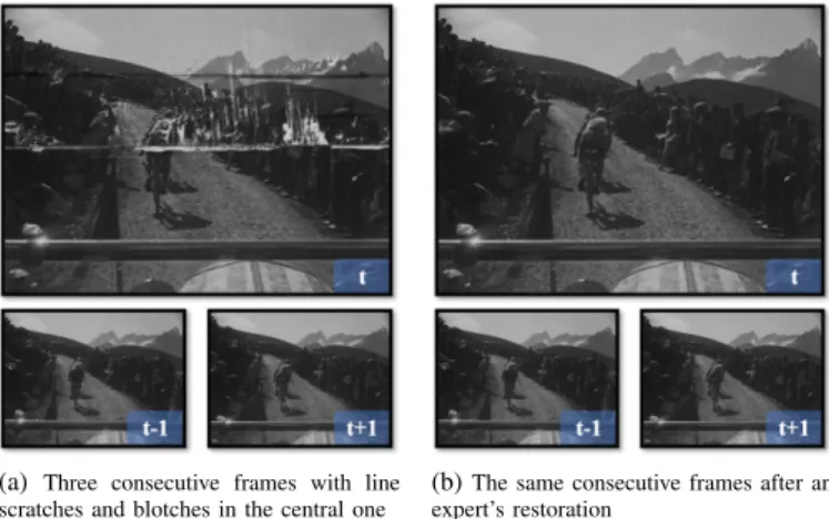
(a) Three consecutive frames with line scratches and blotches in the central one
(b)The same consecutive frames after an expert’s restoration
Fig. 1. Digitized frames from an old movie and its semi-automatic restoration. Our tailored U-Net computes a mask over defect from the original sequence alone (a). The learning step is based on the two sequences (defective (a) and restored (b)) to retrieve a mask of defects resulting from processing on the differences between them.
After reviewing related approaches in Section II, we discuss the creation and analysis of defect mask frames from original and corresponding restored frames in Section III. In Section IV, we train a U-Net from these masks and conduct a series of experiments. We conclude and give perspectives in Section V.
II. RELATEDWORK
The first defect detectors (heuristics) in videos were origi-nally used to detect impulse noise, like the one implemented by [4] for the BBC. It used a threshold on the absolute differences between consecutive frames to detect defects. However, it ignored apparent motion. This is why [5] intro-duced the spike detection index (SDI), with some variations SDIa or SDIx [1], where the absolute differences of motion-compensated frames was used.
A. Line Scratch Detection
The first line scratches detector was proposed by [6], lines being modeled as damped sinusoid contained in the image. First a vertical downsampling and filtering combined with Hough transform were performed, then a Bayesian refinement kept lines that fit the model. This model was generalized in [7] to detect line scratches using wavelet transform and Weber’s law in grayscale movies, then in color ones in [8]. To get better precision, [9] used an algorithm based on over-complete wavelet expansion. Morphological closing was used over an image in [10] to detect the line scratches from difference with the original one, and then tracked theses lines on the others frames with a Kalman filter. This idea of closing was taken up by [11], after having cut the image into several horizontal bands to separate the foreground and the background for better detection. In [12], a thresholded horizontal derivative was applied over the image, then the mean of every column was computed and thresholded again to detect line scratches among all the vertical edges. Hough transform and median filters with variable window size were used in [13]. In addition to the method of [6], [14] examined the values of pixels at the left and the right of the scratch for coherence, to limit false alarm due to edges. Then the different possible lines which were closed were grouped together by a method a contrario. Another idea to limit false alarms was introduced in [15] which consisted in realigning the different mask images following the apparent motion and eliminating those which remained straight lines, since scratch lines did not follow the apparent motion. B. Blotch Detection
In [16], two models of detection were developed: one with a Markov random fields model, and one with a 3D autore-gressive model, associated with their respective heuristics of detection. This MRF model was then used in [17], followed by two refinement stages for false alarm elimination. Both con-straints consisted in enforcing spatial continuity with a MRF and imposing a temporal correlation constraint with a pyra-midal Lucas-Kanade feature tracker. Rank ordered differences (ROD) detector was introduced in [18]. It consisted in taking temporal neighbor pixels in the motion-compensated backward
and forward frames, to compare the distance between them and the current pixel, to their mean value. A simplified version of the ROD detector (SROD) in [19] only dealt with the minimum and maximum values of the neighbor pixels. The SROD detector was also used in [20], where detection was combined with a spatial detector based on morphological area growing and closing. Another application of the SROD detector was introduced in [21], where it was applied in two steps: the first one was the classical one, whereas the second SROD was used with the motion-compensated frames. Detection was performed in [22] as an image segmentation by seedless region growing while introducing a new measure of confidence based on temporal image differences. Other methods required several steps to detect blotches. For instance in [23], the first step consisted in finding potential blotch candidates based on their spatial features. Among these candidates, the real blotches were detected by their temporal intensity discontinuities. A blotch region candidate extraction was performed in [24] using detection of sudden changes in a region using temporal median filtering. Then, these regions were classified as a blotch or not, by finding similarity of the candidate region in the adjacent frames in gradient space, with a histogram of oriented gradients detector.
C. Scratch and Blotch and Deep Learning
To detect blotch and line scratches, [25] experimented a detection method based on cartoon-texture decomposition in the space domain and content-defect separation in the time domain. The distinction between defect or not was handled temporally, using matrix decomposition in a low-rank matrix in addition to a sparse matrix representing the defects. The first deep learning application was dedicated to line scratches detection in [26] using separation of shape and texture. The shape detection was performed by filtering, whereas the texture was classified by a neural network with the edge images as input. A three-steps blotch detection was proposed in [27]: a motion compensation, a SROD detection [19], and classification of all pixels having anomalous values using a convolutional neural network. The same authors tried a three steps approach in [28]. The first step consisted in creating a descriptor containing: the brightness of the three consecutive frames, the same for the motion-compensated frames, the magnitude of the Lucas-Kanade optical flow, and finally the binary templates from local binary pattern operator. Then a SDI detection [5] was performed. Its result and the descriptor became the input for a CNN. For the detection of both blotches and scratches, [29] applied a classification with a CNN encoder-decoder architecture, including concatenation of layers in the encoder part. Then, using the output of the network before the last convolution and softmax for the current frame and the previous frame, a spatial average pooling was performed and a threshold over the Euclidian distance of both results allowed to detect blotches. The line scratches were detected after morphological closing of the network output, and, with shape analysis considerations, defects with their height much greater than their width were kept.
III. DATASETPREPARATION
Our dataset is a movie composed of two sets of around 3,000 grayscale level frames: the first contains original frames, the second is made of the same frames after restoration by an expert (see Fig. 2) with the help of the DIAMANT-Film restoration software1. From a pair of defective and restored
frames, we created masks of the defect areas that we use as the output to be predicted by the neural network.
(a)Defective frame A (b)Defective frame B
(c)Restored frame A (d)Restored frame B
Fig. 2. Examples of defective and respectively restored frames. The different frames in the movie represent texts (a) or natural scenes (b).
A. Mask Creation by Frame Differences and Thresholding The idea to obtain the mask frames here is to compute the absolute difference between the restored image and the defec-tive frame (see Fig. 3), and then to threshold the difference, which is between 0 and 65535 (values for 16-bit images).
(a)Difference of frames A (b)Difference of frames B
(c)Zoom on (a) (d)Zoom on (b)
Fig. 3.Examples of difference frames based on the absolute difference of the defective and restored frames from Fig. 2. While the bigger differences are brighter, the geometric shapes of the computer-assisted restoration software can also be easily recognized.
1https://www.hs-art.com/index.php/solutions/diamant-film
As we can see in Fig. 3, the bigger defects are manually detected and selected by the software user, with simple ge-ometric shapes. Unfortunately, the software operates a copy from the neighbour frames over the whole selection, even if some parts should not be restored. This is why the choice of thresholding is dictated by the compromise between detecting enough defects without over-detecting. With this in mind, we looked at the repartition of the different intensity changes over all the restored pixels in Fig. 4.
Fig. 4. Cumulative proportion of the intensity pixels of defects. The blue threshold is the minimal threshold to detect all absolute differences. With a threshold at 1% of the maximum value (yellow), it represents 30% of all restored pixels. With a threshold at 5% of the maximum value (blue), it represents 6% of all restored pixels.
(a)Difference of frames A: classifica-tion
(b)Difference of frames B: classifica-tion
(c)Zoom on (a) (d)Zoom on (b)
Fig. 5. Classification of the frames differences in Fig. 3 based on the three thresholds of intensity in Fig. 4. All the blue pixels correspond to the minimum threshold and, regarding the original frames in Fig. 2, should not be selected. Considering the letters inside the manual selection as real defects is more difficult to apprehend in spite of the high intensity variation.
With the different thresholds chosen experimentally from the point cloud, we estimated the limit of overdetection to at least 1% of the maximum value, which represents only 30% of the pixels which have been restored. In particular, with a threshold at 5% of the maximum value, we can distinguish the shapes of the different defects (see Fig. 5), even if the correction made on the letters should not be expected. With a higher threshold however, actual defects were not accurately detected. Even with a carefully chosen threshold, there are “holes” in the detection because some restored pixels may have their intensity unchanged.
B. Mask Filling by Morphological Closing
(a)After thresholding (b)After thresholding
(c)After 1 iteration of closing (d)After 1 iteration of closing
(e)After the last iteration of closing (f)After the last iteration of closing
Fig. 6. Morphological closing of the mask frames depending on the thresholding. Every shape is automatically filled with our algorithm that increases the size of the morphological kernels step by step.
To overcome the issue of undetected pixels surrounded by defective pixels, we decided to fill these areas using morphological closure after the thresholding step, to recover spatial connectivity. The kernels of the morphology filters that are used greatly depend on the types of defects present in the images. As previously explained, they are mainly blotches which have globally round shapes, as well as line scratches which are rather vertical lines. The important parameter to know here is the size of closure to perform on the mask frames Imask. To do this automatically, we choose fairly small
starting closure sizes Sline and Sdisk and then progressively
increase each closure size by 1. The stopping condition for the correct closure size is achieved when the number of new
pixels that become mask pixels increases more than in the previous iteration (see Algorithm 1).
Algorithm 1 - Closing shapes in masks
1: Sline← 3, Sdisk ← 2, Imask
2: ∆ ← +∞, ∆∗← #(Imask)
3: while ∆ > ∆∗ do
4: Imask∗ ← closing (Imask, Sline)
5: Imask∗ ← closing (I∗
mask, Sdisk)
6: ∆ ← ∆∗
7: ∆∗← #(Imask∗ − Imask)
8: Imask← Imask∗
9: Sline← Sline+ 1, Sdisk ← Sdisk+ 1
10: end while
The results of our algorithm for closing masks, again with our two same frames, are shown in Fig. 6. It is particularly efficient in filling big defects (see Fig. 6) and linking the different parts of a line scratch.
C. Spatial and Temporal Statistics
Fig. 7. Partitioning of the defects with respect to size and orientation: small (red), vertical (green), big (blue). The two thresholds used are the number of pixels to delimit small defects, and then the orientation to separate vertical defects from other big defects.
To interpret our network results, we organized all the defects from spatial and temporal points of view. Defects are manually partioned to obtain three clusters with the help of two thresholds: small defects, big vertical defects, and other big defects (see Fig. 7). Small defects are separated from other ones according to their relative size in number of pixels. Then the vertical defects are chosen regarding their orientation. With our masks, the results are shown in Fig. 8.
(a)Segmented difference of frame A (b)Segmented difference of frame B
Fig. 8. Examples of masks (with a zoom) with the different colors corresponding to small defects (red), vertical lines or vertical oriented defects (green) and other big defects (blue).
For the temporal analysis, we looked for the different depths of the defect, to know the temporal correlation between certain of them. In particular, we built a frame with the maximum depth of defects for every pixel, along with the whole dataset, with its associated histogram in Fig. 9. Except for some big defects that can be partially overlapped in two successive frames, the only defects with great depth are line scratches. Overall, there are 72% of the pixels with a maximum defect depth of 1 frame, and 95% of them with a maximum of 2 frames. Consequently, using 3 consecutive frames for training should manage a great majority of defects.
(a)Maximum depth defect for every pixel (b)Normalized histogram of (a)
Fig. 9. Maximum temporal depth of the different defects. Defects with the largest depths in (a) are line scratches. Some big shape selections by the expert restorer can also be identified. For 72% of the pixels, the defects have a maximum depth of 1 frame, and it cumulates to 95% with a maximum depth of 2 frames.
IV. EXPERIMENTS ON THENEURALNETWORK
A. Separation of the Dataset
TABLE I
REPARTITION OF THESCENES ANDFRAMES WITH RESPECT TO THETHREETYPES OFSCENES.
Types of scenes Number of scenes Number of frames Text 7 (30%) 931 (31%) Fixed shot 9 (40%) 1105 (37%) Camera motion 7 (30%) 938 (32%)
As a reminder, our dataset consists of a total of 2974 images of 1728×1280 pixels, which are distributed in 23 scenes. The first step was to divide these 23 scenes into three different
types of scenes: scenes with only explanatory or descriptive text, scenes with a fixed shot, and scenes where the camera is moving (see TABLE I).
TABLE II
REPARTITION OF THESCENES, FRAMES ANDPATCHTRIPLETS WITH RESPECT TO THETRAININGSET,THEVALIDATIONSET,
AND THETESTSET.
Dataset Number Number Number of 512×512 of scenes of frames patch triplets Training set 5+7+5 2296 (77%) 27144 Validation set 1+1+1 366 (12%) 4320
Test set 1+1+1 312 (11%) 3672
The second step is to divide the scenes into three different datasets for training, validation and test. For the validation set and the test set, we put one scene of each type, which means three scenes for each of both sets, and 17 for training (see TABLE II). After this separation, other manipulations are needed for statistical analysis and constraints on input and output sizes when implementing the neural network.
B. U-Net Model with Spatio-temporal Patches
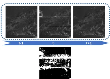
Fig. 10. Input of the U-Net: three temporally consecutive patches of defective frames, and the associated mask of the central patch to operate the comparison with the output of the network.
We decided to use a U-Net, originally designed for the seg-mentation of biometric images [3]. One of the most recurring problems in the use of neural networks in different libraries is that it involves coding input and output image sizes in addition to weights. As a result, the network cannot be used once trained with images of a different size than those used during training. The solution of resizing, which can change the input image ratio, cannot be considered satisfactory. Therefore, We got rid of this constraint by training on patches instead of the whole image. This choice is not a problem in our particular use case, as defects can occur randomly anywhere in the frame; there is no spatial prior to be learned. The prediction step with the image also takes place with the image cut into patches that
overlap. Another consequence of this operation is the increase in the size of the dataset (see TABLE II). Compared to the original U-Net used with only one color image, we used 3 consecutive patches for the input (see TABLE II). The central patch defect mask is used for comparing to the output in the network loss function (see Fig. 10).
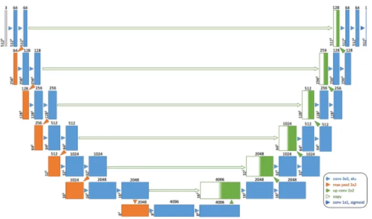
Fig. 11. U-Net architecture used for the detection of defects, with 3 consecutive patches of size 512×512 as input, 7 layers, and 1 patch of the detection of defects as output.
Our U-Net architecture is illustrated in Fig. 11, including a contracting and expansive path as in [3], but with 7 layers in our case. The contracting path consists of the repeated applica-tion of two 3×3 convoluapplica-tions, each followed by an exponential linear unit (ELU) and a 2×2 max pooling operation with stride 2 for downsampling. At each downsampling step the number of feature channels is doubled. Every step in the expansive path consists of an upsampling of the feature map followed by a 2 × 2 convolution that halves the number of feature channels, a concatenation with the corresponding feature map from the contracting path, and two 3 × 3 convolutions, each followed by an ELU. At the final layer, a 1 × 1 convolution followed by a sigmoid is used to map each component feature vector to the associated class. The loss function for the network training is the opposite of the linear approximation of the Dice coefficient, defined as follows:
Loss (yC, yU) = −
2P
i,j
yC(i, j)yU(i, j) P
i,j
yC(i, j) + yU(i, j)
≈ − 2 × T P
(T P + F P ) + (T P + F N ) ∈ [−1, 0] where yC(i, j) ∈ {0, 1} and yU(i, j) ∈ [0, 1] are respectively
the pixels of the defect mask patch from the film expert’s restoration and the output defect mask patch from the U-Net. T P , F P and F N represent respectively the number of pixels counted as true positives, false positives and false negatives. The network was trained using Adam optimizer with a learning rate of 5.10−5. The results in terms of loss function after having predicted all the possible frames in the entire dataset in TABLE III show that, the more complex the scenes are, the harder it is for the network to accurately detect
defects. Indeed, the scenes with only white text with a black background have better scores than fixed shot scenes, which have also better scores than scenes with camera motion. Scores may not appear fully satisfactory. One of the reason is that the restorer’s expertise does not fully constitute a ground truth, typical of this is the over-detection of large manual selections by the restorer.
TABLE III
LOSSFUNCTION WITH RESPECT TO THEDIFFERENTDATASET ANDTYPES OFSCENESCOMPUTED AFTERPREDICTION.
Dataset
Scenes
Text Fixed shot Motion All Training set -0.6252 -0.4564 -0.3629 -0.4323 Validation set -0.8422 -0.2899 -0.2018 -0.2737 Test set -0.8487 -0.5468 -0.2479 -0.4184
As seen in the confusion matrix of TABLE IV, the per-centage of TP / FP / FN is really low compared to the total of pixels involved in the frames. It is quite hard to come to a conclusion concerning what is really well detected or not depending on the quality of the masks we use for training. Yet, all good guess represent 99.58% of all the pixels.
TABLE IV
CONFUSIONMATRIX BETWEEN THEINPUT ANDOUTPUTMASKS.
Input
Output
0 1
0 99.44% 0.10% 1 0.32% 0.14%
We also investigated different sets of inputs to establish how much temporal information is needed for a proper detection. As expected, it is more efficient to consider 3 frames than a single one, since most defects appears on only one frame. More surprisingly, using 5 frames is less effective than 3.
TABLE V
LOSSFUNCTION ON THE TEST SET FOR1TO5FRAMES AS INPUT.
Number of frames 1 3 5 Test set -0.3521 -0.4184 -0.3743
C. Results on the Dataset
The use of geometric shapes to select the different areas to restore implies that the whole selection englobing the defects is replaced by a copy from the neighbour frames, even the good pixels. In spite of the thresholding and morphological closing, we had indicated that the letters of the texts could not be discarded in the mask. Consequently, it leads to many pixels considered as false negatives in Fig. 12. The same problem occurs with the other scenes with the big manual selections which are not completely detected as defect by the network.
(a)Masks of frame A (zoom) (b)Masks of frame B (zoom)
(c)Defective frame A with masks edges (d)Defective frame B with masks edges
Fig. 12. Comparison of the different masks for frames A and B. The true positives are in green, the false negatives in blue, and the false positives in red. The edges of the defects shapes are added on the defective frames with the same color code (i.e. same edges between prediction and manual detection in green).
On the other hand, some defects have unfortunately not been detected by the expert restorer, due to the large number of frames combined to the limited time he can spend on them. Yet, the network manages to outperform the manual detection from restoration in this case and real defects which have not been detected before (see Fig. 13), even if those pixels are considered false positives for the loss function.
Fig. 13. Real defects considered as false positives because of the non-detection by the expert restorer, due to the limitation of the time to spend on restoration.
Despite these visually good results, which are not reflected in the loss function, there are still some limitations. For instance, even if there are really few of them in the dataset, the line scratches detection remains limited by the fact of choosing only 3 consecutive frames (or patches to be precise) in order to detect temporal anomaly in the pixel intensity. Indeed, in the example in Fig. 14, the line scratch is present at the same place in the 3 consecutive frames so the network cannot detect any temporal anomaly. Another limitation of the network concerns the detection of defects when there is a large motion in the scene. Indeed, in this case, the network does not manage to compensate the motion enough to recover the corresponding pixels in the neighbour frames. Consequently, it considers some parts of the frames as blotches, as we can see in Fig. 15.
(a)Frame [time t-1] (b)Frame [time t] (c)Frame [time t+1] (d)Masks [time t]
Fig. 14. Line scratch is not detected (in blue) when its depth is greater than the depth of detection of the network. It is considered as being a part of good pixels (as the white rectangle) since the scratch is present at the same place in all the frames.
(a)Frame [time t] (b)Frame [time t]
(c)Frame [time t+1] (d)Frame [time t+1]
Fig. 15. False detections (in red) which should not be detected, as opposed to Fig. 13. Due to large motion, the network detects them since they look similar to blotches.
D. Comparison with another sequence
We used another sequence from [14] (see Fig. 16) in order to compare the differences between both detections. Even if the line scratches are not entirely detected, which is the aim of the method of [14], almost every other blotch defect is detected.
(a)Newson et al. [14] (b)Ours with contours
Fig. 16. Comparison between line scratches detection of [14] in red (a), and our method of general detection of defects with the contours in blue (b) on the “Star” sequence.
V. CONCLUSION ANDPERSPECTIVES
We introduced a new approach in terms of detection of defects in videos, opening the study for training without the location of these defects, but only with the defective and restored frames. From these frames, we created one possibility for associated masks of defects dataset, based on thresholding the absolute difference between the defective frame and its restoration, followed by an automatic morphological closing step. After a spatio-temporal evaluation of the recovered defects, we trained a U-Net in order to detect the discontinuities in time and space for an automatic detection of defects.
In some cases, we can outperform the manual detection from the restoration with our network. Other cases show that improvements are still possible, either in the refinement of the masks created from the defective and restored images, with data augmentation, or by including motion compensation in our network. However, our approach is here to lay the foundations for more advanced work, and to be included in a larger framework of old movies restoration, in combination with video inpainting techniques [30].
ACKNOWLEDGMENT
We would like to thank our cultural partner, the Cin´emath`eque de Toulouse, which provided us with the data essential to the elaboration of this work, and particularly its expert restorer. This study has been carried out with financial support from the french Minist`ere de la Culture through the program “Services Num´eriques Innovants 2019” and the French Research Agency through the PostProdLEAP project (ANR-19-CE23-0027-01).
REFERENCES
[1] A. C. Kokaram, “On Missing Data Treatment for Degraded Video and Film Archives: a Survey and a New Bayesian Approach,” IEEE Transactions on Image Processing, vol. 13, no. 3, pp. 397–415, 2004. [2] ——, “Ten Years of Digital Visual Restoration Systems,” in Proceedings
of the IEEE International Conference on Image Processing, vol. IV, 2007, pp. 1–4.
[3] O. Ronneberger, P. Fischer, and T. Brox, “U-net: Convolutional Net-works for Biomedical Image Segmentation,” in Medical Image Comput-ing and Computer-Assisted Intervention – MICCAI 2015, ser. Lecture Notes in Computer Science, vol. 9351, 2015, pp. 234–241.
[4] R. Storey, “Electronic Detection and Concealment of Film Dirt,” SMPTE Journal, vol. 94, no. 6, pp. 642–647, 1985.
[5] A. C. Kokaram and P. J. Rayner, “System for the Removal of Impulsive Noise in Image Sequences,” in Visual Communications and Image Processing’92, ser. Proceedings of the SPIE, vol. 1818, 1992, pp. 322– 331.
[6] A. C. Kokaram, “Detection and Removal of Line Scratches in Degraded Motion Picture Sequences,” in Proceedings of the 8th European Signal Processing Conference, 1996, pp. 1–4.
[7] V. Bruni, D. Vitulano, and A. C. Kokaram, “Fast Removal of Line Scratches in Old Movies,” in Proceedings of the 17th International Conference on Pattern Recognition, vol. 4, 2004, pp. 827–830. [8] V. Bruni, P. Ferrara, and D. Vitulano, “Color Scratches Removal using
Human Perception,” in International Conference Image Analysis and Recognition, ser. Lecture Notes in Computer Science, vol. 5112, 2008, pp. 33–42.
[9] J. Xu, J. Guan, X. Wang, J. Sun, G. Zhai, and Z. Li, “An OWE-Based Algorithm for Line Scratches Restoration in Old Movies,” in Proceedings of the IEEE International Symposium on Circuits and Systems, 2007, pp. 3431–3434.
[10] L. Joyeux, O. Buisson, B. Besserer, and S. Boukir, “Detection and Removal of Line Scratches in Motion Picture Films,” in Proceedings of the IEEE Conference on Computer Vision and Pattern Recognition, vol. 1, 1999, pp. 548–553.
[11] T. K. Shih, L. H. Lin, and W. Lee, “Detection and Removal of Long Scratch Lines in Aged Films,” in Proceedings of the IEEE International Conference on Multimedia and Expo, 2006, pp. 477–480.
[12] L. Khriji, M. Meribout, and M. Gabbouj, “Detection and Removal of Video Defects using Rational-Based Techniques,” Advances in Engineer-ing Software, vol. 36, no. 7, pp. 487–495, 2005.
[13] K. Chishima and K. Arakawa, “A Method of Scratch Removal from Old Movie Film using Variant Window by Hough Transform,” in Proceedings of the 9th International Symposium on Communications and Information Technology, 2009, pp. 1559–1563.
[14] A. Newson, P. P´erez, A. Almansa, and Y. Gousseau, “Adaptive line scratch detection in degraded films,” in Proceedings of the 9th European Conference on Visual Media Production, 2012, pp. 66–74.
[15] A. Newson, A. Almansa, Y. Gousseau, and P. P´erez, “Temporal Filtering of Line Scratch Detections in Degraded Films,” in Proceedings of the IEEE International Conference on Image Processing, 2013, pp. 4088– 4092.
[16] A. C. Kokaram, R. D. Morris, W. J. Fitzgerald, and P. J. Rayner, “Detection of Missing Data in Image Sequences,” IEEE Transactions on Image Processing, vol. 4, no. 11, pp. 1496–1508, 1995.
[17] X. Wang and M. Mirmehdi, “Archive Film Defect Detection and Removal: an Automatic Restoration Framework,” IEEE Transactions on Image Processing, vol. 21, no. 8, pp. 3757–3769, 2012.
[18] M. J. Nadenau and S. K. Mitra, “Blotch and Scratch Detection in Image Sequences Based on Rank Ordered Differences,” in Time-Varying Image Processing and Moving Object Recognition, 4, 1997, pp. 27–35. [19] J. Biemond, P. M. B. van Roosmalen, and R. L. Lagendijk, “Improved
Blotch Detection by Postprocessing,” in Proceedings of the IEEE In-ternational Conference on Acoustics, Speech, and Signal Processing, vol. 6, 1999, pp. 3101–3104.
[20] S. Tilie, I. Bloch, and L. Laborelli, “Fusion of Complementary Detectors for Improving Blotch Detection in Digitized Films,” Pattern Recognition Letters, vol. 28, no. 13, pp. 1735–1746, 2007.
[21] M. K. Gullu, O. Urhan, and S. Erturk, “Blotch Detection and Removal for Archive Film Restoration,” AEU - International Journal of Electron-ics and Communications, vol. 62, no. 7, pp. 534–543, 2008.
[22] J. Ren and T. Vlachos, “Segmentation-Assisted Detection of Dirt Im-pairments in Archived Film Sequences,” IEEE Transactions on Systems, Man, and Cybernetics, Part B (Cybernetics), vol. 37, no. 2, pp. 463–470, 2007.
[23] Z. Xu, H. R. Wu, X. Yu, and B. Qiu, “Features-Based Spatial and Temporal Blotch Detection for Archive Video Restoration,” Journal of Signal Processing Systems, vol. 81, no. 2, pp. 213–226, 2015. [24] H. Yous and A. Serir, “Blotch Detection in Archived Video Based on
Regions Matching,” in Proceedings of the International Symposium on Signal, Image, Video and Communications, 2016, pp. 379–383. [25] H. Li, Z. Lu, Z. Wang, Q. Ling, and W. Li, “Detection of Blotch and
Scratch in Video Based on Video Decomposition,” IEEE Transactions on Circuits and Systems for Video Technology, vol. 23, no. 11, pp. 1887– 1900, 2013.
[26] K.-T. Kim and E. Y. Kim, “Automatic Film Line Scratch Removal System Based on Spatial Information,” in Proceedings of the IEEE International Symposium on Consumer Electronics, 2007, pp. 1–5. [27] R. Sizyakin, N. Gapon, I. Shraifel, S. Tokareva, and D. Bezuglov,
“Defect Detection on Videos using Neural Network,” in Proceedings of the XIII International Scientific-Technical Conference “Dynamic of Technical Systems”, ser. MATEC Web of Conferences, vol. 132, 2017, p. 05014.
[28] R. Sizyakin, V. Voronin, N. Gapon, M. Pismenskova, and A. Nadykto, “A Blotch Detection Method for Archive Video Restoration using a Neural Network,” in Proceedings of the 11th International Conference on Machine Vision, vol. 11041, 2019, p. 110410W.
[29] H. Yous, A. Serir, and S. Yous, “CNN-Based Method for Blotches and Scratches Detection in Archived Videos,” Journal of Visual Communi-cation and Image Representation, vol. 59, pp. 486–500, 2019. [30] A. Renaudeau, F. Lauze, F. Pierre, J.-F. Aujol, and J.-D. Durou,
“Alternate structural-textural video inpainting for spot defects correction in movies,” in Scale Space and Variational Methods in Computer Vision, 2019, pp. 104–116.