Delayed-time domain impedance boundary conditions (D-TDIBC)

HAL Id: hal-02057870

https://hal.archives-ouvertes.fr/hal-02057870

Submitted on 5 Mar 2019

HAL is a multi-disciplinary open access

archive for the deposit and dissemination of

sci-entific research documents, whether they are

pub-lished or not. The documents may come from

teaching and research institutions in France or

abroad, or from public or private research centers.

L’archive ouverte pluridisciplinaire HAL, est

destinée au dépôt et à la diffusion de documents

scientifiques de niveau recherche, publiés ou non,

émanant des établissements d’enseignement et de

recherche français ou étrangers, des laboratoires

publics ou privés.

Delayed-time domain impedance boundary conditions

(D-TDIBC)

Quentin Douasbin, Carlo Scalo, Laurent Selle, Thierry Poinsot

To cite this version:

Quentin Douasbin, Carlo Scalo, Laurent Selle, Thierry Poinsot. Delayed-time domain impedance

boundary conditions (D-TDIBC). Journal of Computational Physics, Elsevier, 2018, 371, pp.50-66.

�10.1016/j.jcp.2018.05.003�. �hal-02057870�

O

pen

A

rchive

T

OULOUSE

A

rchive

O

uverte (

OATAO

)

OATAO is an open access repository that collects the work of Toulouse researchers and

makes it freely available over the web where possible.

This is an author-deposited version published in :

http://oatao.univ-toulouse.fr/

Eprints ID : 22901

To link to this article : DOI:

10.10

3 /j.jcp.2018.05.003

URL

http://dx.doi.org/10.1016/j.jcp.2018.05.003

To cite this version : Douasbin, Quentin and Scalo, Carlo and Selle,

Laurent and Poinsont, Thierry : Delayed-time domain impedance

boundary conditions (D-TDIBC) (2018), Journal of Computational

Physics, vol. 371, n°10, pp.50-66

Any correspondance concerning this service should be sent to the repository

administrator:

staff-oatao@listes-diff.inp-toulouse.fr

Delayed-time

domain

impedance

boundary

conditions

(D-TDIBC)

Q. Douasbin

a,b,

∗

_,

_{C. Scalo}

c

_,

_{L. Selle}

a,b

_,

_{T. Poinsot}

a,b

a_{UniversitédeToulouse,INPT,UPS,IMFT,31400Toulouse,France} b_{CNRS,IMFT,31400Toulouse,France}

c_{SchoolofMechanicalEngineering,PurdueUniversity,WestLafayette,IN47907,USA}

a

b

s

t

r

a

c

t

Keywords:

Impedanceboundarycondition Timedelay

Characteristicboundaryconditions NSCBC

Computationalaeroacoustics Thermoacoustics

Definingacousticallywell-posed boundaryconditions isoneofthemajornumerical and theoretical challenges in compressible Navier–Stokes simulations. We present the novel Delayed-Time DomainImpedanceBoundaryCondition(D-TDIBC) technique developed to imposeatimedelaytoacousticwavereflection.UnlikeprevioussimilarTDIBCderivations (Fungand Ju,2001–2004 [1,2], Scaloetal., 2015 [3] and Lin etal.,2016 [4]), D-TDIBC reliesonthemodelingofthe reflectioncoefficient. Aniterativefitisused todetermine the model constants along witha low-pass filtering strategyto limitthe model to the frequencyrangeofinterest.D-TDIBCcanbeused totruncateportionsofthedomainby introducingatimedelayintheacousticresponseoftheboundaryaccountingforthetravel timeofinviscidplanaracoustic wavesinthetruncatedsections:itgivestheopportunity to save computational resources and to study several geometries without the need to regeneratecomputationalgrids.TheD-TDIBCmethodisappliedheretotime-delayedfully reflectiveconditions.D-TDIBCsimulationsofinviscidplanaracoustic-wavepropagatingin truncatedductsdemonstratethatthetimedelayiscorrectlyreproduced,preservingwave amplitudeandphase.A2Dthermoacousticallyunstablecombustionsetupisusedasafinal testcase: DirectNumericalSimulation(DNS) ofanunstable laminarflameisperformed using a reduced domain along with D-TDIBC to model the truncated portion. Results are in excellent agreement with the same calculation performed overthe full domain. The unstable modes frequencies, amplitudes and shapes are accurately predicted. The resultsdemonstratethatD-TDIBCoffersaflexibleandcost-effectiveapproachfornumerical investigationsofproblemsinaeroacousticsandthermoacoustics.

1. Background

Direct NumericalSimulation (DNS)orLargeEddy Simulation (LES)havebecome standard approachesforhigh-fidelity simulationsofunsteadycompressibleflows.Inmanycases,accurateflowpredictionscanbeobtainedonlyifthereflection oftheacousticwavesattheboundariesispreciselydefinedand/orcontrolled[5–8].Impedanceisawidely-usedquantityto characterizethereflectionofacousticwavesatboundaries;itisnaturallydefinedinthefrequencydomainwhereasDNS/LES areperformedinthetimedomain.Numericalmethodspermittingtheimpositionofimpedanceboundaryconditions(IBCs)

*

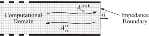
Correspondingauthorat:UniversitédeToulouse,INPT,UPS,IMFT,31400Toulouse,France.

Fig. 1. Orientation of ingoing and outgoing acoustic waves Ainn and Aoutn with respect to an Impedance Boundary (IB) with outward pointing normaln.E

in time domain solvers fallunder the categoryof TimeDomain Impedance Boundary Conditions (TDIBC).While existing TDIBCmethods [1–4,9–14] havedemonstratedtheirabilitytoachievesuchgoal,onecasehasnotyetbeconsideredinthe ComputationalAeroacoustics(CAA)community:apure timedelay.DevelopingDelayed-TimeDomainImpedanceBoundary Conditions(D-TDIBC),i.e. aTDIBCallowingtoimposeatimedelay,isthegoalofthepresentwork.

The proper implementationofboundary conditionsis criticalforthe stability ofthe numericalsolution. Forexample, directlyimposingmeanvaluesofvelocityorpressureattheboundaryleadstocompletereflectionofacousticwaves,hence leadingtoanartificialincreaseindisturbanceenergy.

Acoustic waves are the manifestation of perturbations around a mean state: the pressure field, for instance, can be expressedas p

(

t

)

₌

p0

+

p′

(

t

)

,wherep0 isthemeanpressureandp′

(

t

)

istheacousticperturbation.Inthepresentwork,

thetimeharmonicbehaviore+iωt _{isassumed,yielding theconvention}

_{φ (}

_t

₎

= ℜ(φ(

ω

)

e+iωt

₎

_{foragenericperiodicfunction}

φ

′

(

t

)

oscillatingwithangularfrequency

ω

.ThecorrespondingFouriertransformconventionreads:

φ (

ω

)

₌

+∞

Z

−∞

φ (

t

)

e−iωtdt (1)

with

F

beingtheFourieroperator

φ (

ω

)

= F (φ

′

₍

_t

₎₎

_{,yieldingthecomplexfluctuationamplitude}

_{φ (}

_ω

₎

_.

Thespecificimpedance Z_∗

(

ω

)

isdefinedinthefrequencydomainasthenon-dimensionalratioofcomplexpressureand thevelocitycomponentnormaltotheboundary [15]:

Z_∗

(

ω

)

₌

1

ρ

0c0

p

(

ω

)

E

u

(

ω

)

_{· E}

n (2)

where

ρ

0 andc0 are themeandensityandspeedofsound,respectively. Z_∗

(

ω

)

isafrequency-dependentcomplex-valued function, which iscommonlyused to characterizethe response ofan acoustic element.It is unbounded,contrary tothe reflectioncoefficient R andthewallsoftnessS,whicharedefinedas:

R

(

ω

)

₌

1

−

Z∗

(

ω

)

1

₊

Z_∗

(

ω

)

,

S

(

ω

)

=

R

(

ω

)

+

1

.

(3)

Unlikethespecificimpedance Z_∗,boththereflectioncoefficient R andthewallsoftness S areboundedinamplitude (for passive acoustic elements),making them theworking variableof choice incomputations.Fig. 1 illustrates the definition ofthe outgoingandingoing acousticwaves, Aout_n and A_nin,orientedinthe samedirectionofandopposite totheoutward normaln.

_E

Followingthisconvention,theoutgoingandingoingcharacteristicwavesaredefinedas:

Aout_n

(

ω

)

_{= E}

u

(

ω

)

_{· E}

n

₊

p

(

ω

)

ρ

0c0

,

Ain_n

(

ω

)

_{= E}

u

(

ω

)

_{· E}

n

₋

p

(

ω

)

ρ

0c0

(4)

CombiningEqs. (2) and(3) yields:

R

(

ω

)

₌

A in n

(

ω

)

Anout

(

ω

)

(5) S

(

ω

)

₌

A in n

(

ω

)

+

Aoutn

(

ω

)

Aoutn

(

ω

)

(6)

Impedance,reflectioncoefficientandwallsoftnessaredefinedinthefrequencydomainwhereasDNS/LESareperformed inthetime domain.However, inorderfortheTDIBCtobe physicallyadmissible,thefollowingthreemathematical condi-tionsmustbefulfilled,asstatedbyRienstraetal. [11]:

1. Reality: Thecharacteristicwavesimposedinthetimedomainshouldbepurelyreal.Suchapropertycanbeensuredin thefrequencydomain,forinstanceinthereflectioncoefficient,if:

R∗

(

₋

ω

)

₌

R

(

ω

)

(7)

2. Causality: Anyprocessshould havea zero-responsebefore itistriggered.Mathematically,sucha conditionisfulfilled if1:

ℜ(

pi

)

≤

0 for i

∈ [

1

;

npoles

]

(8)

where pi representstheith complexpoleofthe reflectioncoefficient R

(

ω

)

prolongedto theLaplace plane and

ℜ(·)

denotestherealpartoperator.

3. Passivity: The reflected wave amplitude should be lower or equalthan the amplitude of the incident wave. This is fulfilledfor:

|

R

(

ω

)

_{| ≤}

1 (9)

Shouldoneoftheseconstrainsbe violated,theimpositionofTDIBCisexpectedtocontributetonumericalinstabilities. Itishenceimperativetobearinmindsuchmathematicalconstraintswhenmodeling R

(

ω

)

(or S

(

ω

)

).

Thetimedomainequivalentof R

(

ω

)

isobtainedbyuseoftheinverseFouriertransformR

(

t

)

_{= F}

−1

(

R

(

ω

))

andS

(

t

)

₌

F

−1

₍

S

(

ω

))

.When dealing with the imposition of acoustic propertiesat a boundary condition, both the outgoing wave

Aout_n

(

t

)

(evaluatedfromthecomputationaldomain)andthereflectioncoefficientR

(

ω

)

(respectivelythesoftnesscoefficient) are known.However, the ingoing wave A_nin

(

t

)

is unknown andhasto be evaluated fromthe valuesof Aout_n

(

t

)

and R

(

ω

)

(respectively S

(

ω

)

).ThiscanbedonebyrecastingEq. (5) (respectivelyEq. (6))andtakingitsinverseFouriertransform.As theinverseFouriertransformof aproduct yields aconvolution integral [16,17],Eqs. (5) and (6) can beexpressed inthe timedomainasfollows:

Ain_n

(

t

)

₌

t

Z

0 R

(

τ

)

Aout_n

(

t

₋

τ

)

d

τ

(10) Ain_n

(

t

)

_{= −}

A_nout

(

t

)

₊

t

Z

0 S

(

τ

)

Aout_n

(

t

₋

τ

)

d

τ

(11)

wheretheboundsoftheintegralsinEqs. (10) and(11) arereducedto

τ

_{∈ [}

0

,

t

_]

aswe assumethat S

(

t

)

, R

(

t

)

, A_nin

(

t

)

and

Aoutn

(

t

)

aredefinedontheintervalt

∈ [

0

,

+∞]

.Forthecausalityconstraintnottobeviolated, Ainn

(

t

)

mustdependonlyon

pastandpresentvaluesof R

(

t

)

(respectively S

(

t

)

)and A_nout

(

t

)

butcannotdependonfuture values.

TheseassumptionsrestricttheboundsoftheconvolutionintegralsasitisthecasewhenusingthecausalinverseLaplace transform [18,19].Noncoincidentally,the conversionfromthefrequency domainto timedomain asdonein mostTDIBC technique(seesection3)requirestheformalprolongationofthesupportoftheFouriertransform,restrictedtoareal-valued frequency

ω

,tothecomplexdomain.Thisisstepishiddenbyan abuseofnotation wherethequantity i

ω

isintended as complexandhencefollowingtheformalismofLaplacetransforms(s

₌

i

ω

).

Althoughmathematically equivalent to Eqs. (5) and (6), Eqs. (10) and (11) are not directly applicable in high-fidelity compressiblesolvers becausethedirectevaluationoftheconvolution integralrequiresalargeamountofmemory.Indeed,

Aout_n

(

t

)

andR

(

t

)

needtobestoredateveryiterationandeachboundarynodeorface.Forsimplegeometries,Nottin [20,21] hassolvedEq. (10) directly.IncomputationallyintensiveframeworkssuchasDNS/LESofturbulent flows,amoreefficient compact-in-timemethodisrequiredfortheevaluationof Ain_n

(

t

)

,asshowninrecentpapersonthistopic [1–4,14,22–26].

Advancesintime domainimpedanceimposition intheelectromagneticcommunityhavedrivennovel acoustic bound-aryconditionsforcomputational aeroacoustics [9,10,27,28]. Özyoruk et al. [10,27,29] and Tam andAuriault [9] havefirst developed formulations of TDIBC based on the z-transform anda Laurent series development of the impedance in the frequencydomain resultingina time domain OrdinaryDifferential Equation (ODE)problem. Numerical instabilitieswere observedbyÖzyoruk etal. [10,27,29] anddiscussedbyTamandAuriault [9].Recentworkonthistopicsuggeststhatthese instabilitiesareduetotheillposednessoftheimpedanceboundarycondition whencoupledwithMyers’slipflowvelocity condition [11,30].

FungandJu [1,2] haveproposedacausalformulationofTDIBC basedonthewall softnessS.Asall Recursive Convolu-tionmethods (RC),Fung andJu’smethod evaluates theconvolution integral (Eq. (11))ina low-storage manner.Toavoid recomputingthewholeconvolutionintegralatalltimes(whichwouldbeincreasinglycostlyintime)itisevaluatedby(1) computingthechangeofthe convolutionintegral’svalue overa time stepand(2)store theupdated value.Such method bypassestheneedtostorethetime historyof S

(

t

)

and Aout_n

(

t

)

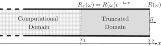
asonlythevalueoftheconvolution integralcalculatedup totheprevious timestepneeds tobestored. Themethodreliesonpartialfractionmodelinginthe frequencydomain,as discussedinSec.3.1.Thismodelingreliesinidentifyingthe polesandresiduesofa complexfunction–thewall softness coefficient S inFung andJu’s case. The update ofthe convolution integral isdone by solving Eq. (11) over a time step sothat a low-costevaluationis possibleusinga trapezoidalquadraturerule.Fung andJu’sformulationhasbeenapplied

Fig. 2. Typicalcasewherethecomputationaldomaincanbecutatx=x1.Thepropagationofacousticwavesinthetruncatedportion(betweenx1andx2)

isaccountedforbythedelayedreflectioncoefficientRτ(Eq. (12)).

toone-dimensionalinviscidEulercalculations [1,2] and,morerecently,appliedinfullycompressibleNavier–Stokes simula-tions [3,4],withsomemodificationsrequiredtoensurenumericalstabilityoftheimplementation,namelysettingthephase parametertozero(seesection6.3inLinetal.[4]).

Anotherlow-storagealternativetoRCmethods,isreferredtointheliteratureastheAuxiliaryDifferentialEquation(ADE) method.Suchmethodalsoreliesonpartialfractionmodelingbutitinvolvesthetemporalintegrationofasetoffirst-order ordinarydifferentialequationsderived fromthepolesandresiduesequivalenttotheconvolutionintegralsinEqs. (10) and (11).Themajoradvantageofthismethodisthatthesametime-marchingaccuracyoftheNavier–Stokessolvercanbeused for theTDIBC, thus ensuring consistencyin the overall time accuracyorder. Acomparison betweenthe ADEand theRC methodscanbefoundinDragnaetal. [31].TheADEmethodwasalsousedtoimplementaTDIBCinTroianetal. [32].

Inthecombustioncommunity,a state-spaceapproach,calledCharacteristic Basedstate-spaceBoundary Condition (CB-SBC), hasbeen developedby Schuermans etal. [33], Kaess et al. [22] and Jaensch et al. [24], andusedin Navier–Stokes simulations [14,22,24,26].CBSBCreliesoncontrol theoryoflineartime-invariant(LTI)systemsto buildareflectionmodel through first-orderdifferentialmatrix equations [24]. Twoformulations ofCBSBCwere proposed. Thefirst formulationof CBSBC isa state-spaceapproachunder theso-calledcontrollablecanonical form,i.e.based onthemodeling ofatransfer functionasarationalpolynomial.ThesamemodelingprocedurewasusedbyZhongetal. [13] tomodeltheimpedance.The transfer functionrepresentsthebroadband reflectioncoefficient.Similarlyto FungandJu’s method [1,2],thisformulation ofCSCBCaimsatimposingwavereflectionwithnear-zerotimedelay as,forpracticalreasons,itfailstohandlepuretime delay. Indeed,for thepure time delay imposition problem, CSCBC modeling requires a highnumber ofPadé polynomial coefficientsleadingtoill-conditionedmatrices,makingthisformulationdifficulttouse.AsecondformulationofCBSBCwas proposedbyJaensch etal. [14] specificallytoimposepuretimedelays.ThisapproachconsistsinimplementingaLinearized Euler Equation(LEE) solver foreach of the impedanceboundary conditionsin the domainandperforming thetemporal integrationusingafirst-orderupwindscheme.The1DspatialdiscretizationneededbytheLEEsolverisdonebystoringin memorya statematrixofdimension 2N

_×

2N,andthreematricesofdimension 2

_×

N,where N isthenumberofnodes consideredinthespatialdiscretization.Intheirwork,Jaensch etal. [14] haveshownthattoimposeapuretime delayfor a 1D wave propagationproblem itwas necessary toconsider a numberofnodes ashighas N

₌

1000 in orderto avoid acousticenergydissipation.

Inthiswork,areformulationofFungandJu’smethodbasedonthereflectioncoefficientispresentedandusedtoimpose puretimedelaysinDNS/LES.AlthoughmathematicallyequivalenttotheTDIBCmulti-oscillatorstrategyusedbyLin etal. [4], whichtargetsthewallsoftness,theformulationadoptedinthepresentworkfocusesonthereflectioncoefficientasitisa morenaturalandconvenientchoiceforproblemswheredelayedtemporalresponsesofacousticboundariesareofinterest. Section 2willpresentthe definitionofdelayedreflection,which allowstruncating longportions ofthecomputational domains.Section 3willintroducetheTDIBCformulationusedinthisworkandthefittingtechniquenecessarytomodela delayedreflectioncoefficient. InSec.4 D-TDIBCwillbe usedto imposea timedelay ina 1D wavepropagationtest case. Finally,inSec.5a2DthermoacousticallyunstablecombustionchamberisstudiedviaDNS,usingtheD-TDIBCtechniqueto reducethedomainsize.

2. Problemformulation:delayedimpedanceboundaryconditions

In manysimulationsofindustrial systems,longitudinalwavespropagate overelongated portions ofthecomputational domain(e.g.intheexhaustpipe ofa carengine,inthechimneyonan industrialfurnace or,ingeneral, forductsofboth constant sectionandspeedofsound),merely resultinginatimelagoftheacousticresponse.Insuchcasesthe computa-tionaldomaincanbesignificantlyreduced,byreplacingsuchelongatedportionswithaboundarycondition accountingfor thetemporaldelayassociatedwiththeacousticwavepropagationtime.

Fig.2showsanacousticprobleminwhichtheportionfromx1tox2istruncated(greyarea).Inthiscomputationalsetup,

theboundaryconditionlocatedinx

₌

x1 mustaccountfortheacousticpropertiesofthetruncateddomain.Thisispossible

iftheboundary condition atx

₌

x1 imposes atimedelay tothewave reflectionlocatedatx

=

x2: theresultingreflection

coefficient is calleddelayedreflectioncoefficient [7,34]. Assuming planar and linearwave propagation yields the following expressionforthedelayedreflectioncoefficientRτ :

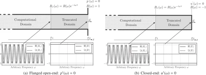
Fig. 3. Acousticvariablesfortwocanonicallimitcases:(a)theflangedopen-end,and(b)theclosed-end(hardwall)cases.Bothconfigurationsarefully reflectiveandhaveapurelyrealreflectioncoefficientR atallfrequenciesinx=x2.Thetruncationofthegreyareascanbemodeledbytheimpositionof

atimedelayτ.TheresultingdelayedreflectioncoefficientRτatx=x1iscomplex.Atthebottomofthefigurebothreal(solidlines)andimaginaryparts

(dashedlines)ofRτ andR areshownforbothcases.

where

τ

is the total time delay (i.e. the time required by a wave to travel from x1 to x2 and back) and i

=

√

−

1 is

the imaginaryunit. In thisformulation ofthe delayed reflectioncoefficient, it is assumed that the basepressure in the truncatedsectionisuniform. Andifferentformulationshouldbederivedforcaseswhere,forexample,significantpressure dropsarepresentinthetruncatedsection.

Fig.3illustratestheimpactofanarbitrarytimedelay

τ

ontwoclassicallimitcases:theflangedopen-end, i.e.p

(

ω

)

=

0 (Fig. 3(a)), and the closed-end, i.e. u

(

ω

)

=

0 (Fig. 3(b)). These cases have purely real reflection coefficients R

(

ω

)

at the acoustic boundary located in x

₌

x2. Forall frequencies

ω

, the flanged open endcorresponds to a reflection coefficient

of R

(

ω

)

=

1 and the closed end to R

(

ω

)

= −

1. The delayed reflection coefficient Rτ

(

ω

)

becomes complex-valued and frequency-dependenteventhough R

(

ω

)

ispurelyrealandfrequency-independent.

Inthiswork webuild uponthemulti-oscillator TDIBCmethodologyofFungandJu [2], withthephase-parameter cor-rectionbyLinetal.[4], tocreatea novelTDIBCformulation, calledDelayed-TimeDomain ImpedanceBoundaryCondition (D-TDIBC),relying onthedeterminationofthepartialfractionrepresentation(viapolesandresidues)ofthedelayed com-plexreflectioncoefficient,asoutlinedinSec. 3.1.Itisimportantto notethat byadoptingFungandJu’s formalism,which focuseson the causal reconstruction of the softness (or absorption) coefficient, it is indeedappropriate to talk about a multi-oscillatorfittingstrategy,wherethefittedsoftnessisthelinearsuperpositionofthesoftnesses ofvariouscausal os-cillators,whichcan beeachrepresentativeofrealacousticallyabsorptivepanels;ontheother hand,thedecompositionof thereflectioncoefficientinpartialfractionsasdone inthepresentwork (seeEq.(13))isnot tiedtoaparticularphysical interpretation.Dueto thepeculiarmathematical natureofthe delayedcomplexreflectioncoefficient (Eq. (12),plottedin Fig.3),exhibitingperiodic variationsin thefrequencydomain,theproposed D-TDIBCstrategy wasdevelopedto handlea largenumberofpolesandresidues.Whilethefocushereinisonthereflectioncoefficient R,thesamefittingmethodology outlinedinSec.3canbeextendedtothewallsoftnessS.

3. Methodology

3.1. Timedomainimpositionofcomplexreflectioncoefficient

ThedirectnumericalintegrationofEq. (10) does,inprinciple,allowtoimposeacomplexreflectioncoefficientinthetime domain;however,thisresultsinrapidlyunsustainablememoryandCPUcosts,especiallyinDNS/LESsimulations.Building uponthemethodologiesofFungandJu [1,2],Scalo etal. [3] andLin et al. [4], weapproximateagenerictarget reflection coefficient R

(

ω

)

withthereflectioncoefficientoftheboundarycondition RBC expressedasasumofrationalfunctions:

R

(

ω

)

_≃

RBC

(

ω

,

n0

)

=

2n0

X

k₌1

µ

k i

ω

−

pk (13)

whereRBC

(

ω

,

n0

)

isthereflectioncoefficientmodelandthepolesandresidues(pk,

µ

k)mustcomeasn0 conjugatepairs:

p2k

=

p∗2k−1

;

µ

2k

=

µ

∗2k−1

;

k

∈ [

1

;

n0

]

(14)

Theseconjugatepairsensurethatthereflectioncoefficient R isreal-valuedinthetimedomain.Thetimedomainequivalent ofEq. (13) is:

RBC

(

t

,

n0

)

=

2n0

X

k₌1

µ

kepktH

(

t

)

(15)

where the Heaviside function H

(

t

)

indicates that the causality constrained is fulfilled. The time-domain incoming wave value A_nin

(

t

)

correspondingtoRBC

(

ω

,

n0

)

isobtainedbysubstitutingEq. (15) intoEq. (10) yields

Ain_n

(

t

)

₌

2n0

X

k₌1 t

Z

0

µ

kepkτAnout

(

t

−

τ

)

d

τ

=

2n0

X

k₌1 Ik

(

t

)

(16)

comprising2n0 convolutionintegralscalledIk,whichcanbesplitintotwocontributions [1,2]:

Ik

(

t

)

=

Ik

(

t

− 1

t

)

epk1t

+

µ

k t

Z

t−1t epkτ_Aout n

(

t

−

τ

)

d

τ

(17)

Equation (17) showsthateachIk

(

t

)

canbeevaluatedrecursively:thefirsttermcorrespondstothetemporalintegrationover

theinterval

τ

_{∈ [}

0

,

t

_{− 1}

t

_]

andthesecond termtothetemporalintegrationovertheinterval

τ

_{∈ [}

t

_{− 1}

t

,

t

_]

.Itprovides alowmemorystoragemethodtocomputetheingoingwave Ain_n

(

t

)

.Theonlyquantitiesneededtobestoredare Ik

(

t

− 1

t

)

and Aout_n

(

t

)

.TheresultingCPUandmemorycostdoesnotincrease withthenumberoftime steps,andthecomputational overheadassociatedwiththeintegralinEq. (17) overatimestep

1

t isminimal.

WeadoptatrapezoidalquadratureruleforthediscretizationoftheintegralinEq. (17),yielding[1]:

Ik

(

t

)

=

Ik

(

t

− 1

t

)

epk1t

+

α

kAoutn

(

t

)

+ β

kAoutn

(

t

− 1

t

)

(18)

α

k

=

µ

k

Ã

epk1t

₋

₁ p2_k

1

t

−

1 pk

!

; β

k

=

µ

k

Ã

epk1t

₋

₁ p_k2

1

t

−

epk1t pk

!

(19)

It should be notedthat Eqs. (18) and (19) limitthe overall temporalaccuracy order to second order;this can be over-comebydevelopinganalternativetimeintegrationstrategybasedontheAuxiliaryDifferentialEquation(ADE)method(see Background),whichisoutofthescopeofthepresentpaper.

TheinitialvaluesofIk

(

t

)

andAoutn aresettozerointhesimulations [1–4].However,onecanmakeacheckpointrestart

by initializingtheIk

(

t

)

usingstoredvaluesfromaprevious simulation.UsingEqs. (18) and(19),compleximpedancescan

beimposedinDNS/LESsolvers.

Themethodologytodeterminethemodelinputs

(

µ

k

,

pk

)

isnowpresented.

3.2. Multi-PoleModeling

As discussedinSec. 3.1,inorder toimposethereflectioncoefficient R

(

ω

)

weneed todeterminethe setofpolesand residues

(

pk

,

µ

k

)

.Thereisnoevidenceoftheuniquenessofthesolutionforasetof

(

µ

k

,

pk

)

.Weproposehereamethod

to determinethepolesandresiduesthatisviablewhenmodeling delayedreflectioncoefficients (Eq. (12)).It isatedious taskasthedelayedreflectioncoefficient Rτ

(

ω

)

hasmanyzerosintroducedbythecomplexexponentiale−i_{ωτ .Themethod}

consistsinaniterativeleast-squarefit.Ateachiteration,arationalfractionisaddedtothemodeluntilthemodelreflection coefficient RBC

(

ω

)

convergestothedesiredreflectioncoefficientR

(

ω

)

.

Inordertodevelopthisfittingmethod,wewillfirstdescribethepropertiesoftherationalfractionsinEq. (13).

3.2.1. PoleBaseFunctionproperties

The reflectioncoefficient of the boundarycondition RBC

(

ω

,

n0

)

isa sumof n0 rationalfractions, calledthe Pole Base

Functions(PBF),denoted Rk: RBC

(

ω

,

n0

)

=

n0

X

k=1 Rk

(

ω

)

=

n0

X

k=1

·

µ

k i

ω

−

pk

+

µ

∗_k i

ω

−

p_k∗

¸

|

{z

}

Pole Base Function

(20)

Equation (20) canbe recastby expressingthe polesandresidues intheir algebraic forms,i.e.as

µ

k

=

ak

+

ibk and pk

=

ck

+

idk withak

,

bk

,

ck

,

dk

∈ R

.EachRkiscausalifck

<

0 [11,35].

Although Fung & Ju [2] suggested that the phase parameter Bk

=

bkdk

+

akck could be not null, Lin et al. [4] have

experienced spurious oscillations, leading to unstable numerical simulations, when the parameter Bk was unconstrained

Bk

6=

0.AlthoughtheTDIBCofinterestisbasedonthereflectioncoefficient R ratherthanonthewallsoftnesscoefficient

S,similarbehaviorwasobservedinpreliminarynumericaltrialsbytheauthors.Thus,thephaseparameterwasconstrained to Bk

=

0,i.e.bk

= −

akck

/

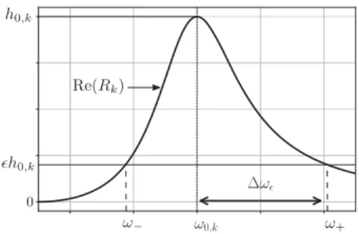
dk,leadingto:

Fig. 4. RealpartofatypicalPBFRk(Eq. (21)).Threepropertiesarevisualized:ω0,k,h0,kand1ωǫ.Attheresonantangularfrequencyω0,k,therealpart

ofRkismaximum.Thepeakheight h0,kisthevalueofRk(ω)atω=ω0,k.Foragivenpercentageǫ(ǫ∈ [0,1]),thehalf-width1ωǫisdefinedonthe

right-hand-side.ω₋andω₊arethesolutionsoftheequationℜ(Rk)=ǫandareusedtodefinethewidth.

Rk

(

ω

)

=

2aki

ω

−

ω

2

₋

_2c

ki

ω

+

¡

c2_k

+

d2_k

¢

(21)

TherearethreedegreesoffreedominEq. (21),namelyak,ck anddk.Theobjectiveofthissectionistolinkthesedegrees

offreedomtothepropertiesofthePBF.

AtypicalPBFispresentedinFig.4wherethreepropertiesofthePBFcanbeidentified:

ω

0,k,h0,k and

1

ω

ǫ .

ω

0,k isthe

frequencywheretherealpartof Rk is maximum:itisreferred astheresonantfrequency. h0,k isthe peakheight, thatis,

thevalueof Rk

(

ω

)

at

ω

=

ω

0,k.The lastpropertyshowninFig.4isthehalf-width

1

ω

ǫ definedfora givenpercentage

ǫ

ofh0,k (

ǫ

∈ [

0

,

1

]

).BecausethePBF isnotsymmetric,atagivenpercentage

ǫ

,two half-widths

1

ω

ǫ canbedefined:one ontheleft-handside (using

ω

₋)andoneontheright-hand side(using

ω

₊). Achoiceismadetoconsideronlytheright half-widthshowninFig.4,henceoverestimatingthewidth.

Onecanshowthat [3,4]:

ω

2_0,k

₌

c_k2

₊

d2_k (22)

Equation (22) givesa first constraint, sayon dk. Injecting Eq. (22) intoEq. (21) andevaluating the resultingequation at

ω

₌

ω

0,k yields:

Rk

(

ω

0,k

)

=

h0,k

= −

ak

ck

(23)

UsingtheconstraintsinEqs. (22) and (23), Rkbecomes:

Rk

(

ω

)

=

2h0,kcki

ω

ω

2

+

2cki

ω

−

ω

20,k

(24)

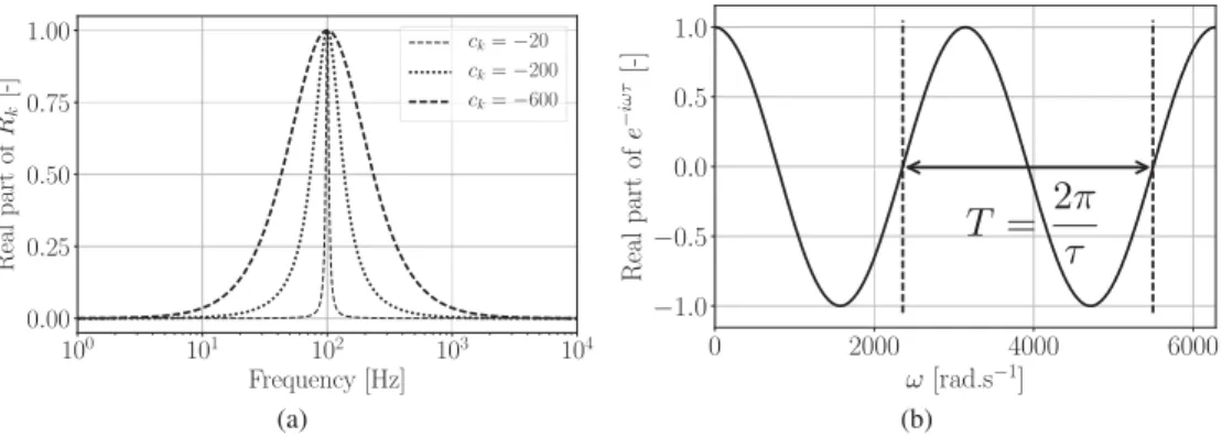
InEq. (24),ckisthe onlyremainingdegreeoffreedom.Fig.5(a)illustrates itseffectonthewidthofaPBF Rk forapeak

heighth0,k

=

1 attheresonantfrequency f0,k

=

ω

0,k

/

2

π

=

100 Hz.Inthecaseofapuredelay thewidthisknown: R

(

ω

)

isaperiodicfunctionofperiodT

₌

2

π

/

τ

(Fig.5(b)).AsshowninFig.5(a),therealpartofRkgoestozerosfor

ω

<<

ω

0,k

and

ω

>>

ω

0,k.A consequenceofthispropertyisthat asingle PBFcan fita singlepeak betweentwoconsecutivezeros.

Forthepuredelay thefrequencyrangebetweentwoconsecutivezerosis T

/

2.Toadjustthewidthtothepuredelay case, weneedtofindthevalueofck foragiven

ǫ

suchthat:

ℜ

·

Rk

µ

ω

0,k

+

T 4

¶¸

= ℜ

h

Rk

³

ω

0,k

+

π

2

τ

´i

=

ǫ

(25)

where

_ℜ(·)

and

_ℑ(·)

aretherealandimaginaryparts,respectively.Solving forckinEq. (25),weobtainthecriterionfora

giventimedelay

τ

:

ck

(

ǫ

,

ω

0,k

)

= −

τ ω

0,k

+

π₄ 2

π ω

0,k

+

τ

r

ǫ

1

₋

ǫ

(26)

Equations (22), (23) and (26) give constraintsallowing tocontrol the heightandthe widthofa PBFfor anyresonant angular frequency

ω

0,k. These constraints are used in the algorithm allowing the determination of the set ofpoles and

residues(pk,

µ

k)presentedinthenextsection.

3.3.IterativeMulti-PoleModelingTechnique

NowthatthepropertiesofasinglePBFareknown,itispossibletogobacktoEq. (20) whereasumofn0 PBFsareused

tomatchareflectioncoefficient R

(

ω

)

.Inthecaseofpure delay,it isatedioustaskasthe complexexponentialfunction, introducedbythetimedelay(seeEq. (12)),hasalargenumberofzeros.

Fig. 5. (a)Influenceoftheckparametersfor f0,k=21πω0,k=100 Hz andh0,k=1.(b)RealpartofapurelydelayedreflectioncoefficientRτ foratime

delayτ.Therealpartisaperiodicfunction(cosine)ofperiodT₌2π τ.

Acommonpracticetoobtainthemulti-poleapproximationofacomplexfunctionistousetheVectorFittingmethod [36,

37].It was usedtomodelTDIBC usingpartialfractionsby severalauthors [12,31,38–40].However, preliminarytestshave shown onlylimited resultswhen applied to complex exponentials asconvergence could not be reachedwhen modeling puretimedelays.Totacklethisissueaniterativefittingtechniquehasbeendevised.

The least-squarefit algorithmisused tominimize thedistanceofthe target function R

(

ω

)

tothefit function RBC

(

ω

)

(Eq. (21))onbothrealandimaginaryparts.Thegloballeast-squareresidual

ξ

isdefinedasthesumofthesquareddistance betweenR

(

ω

)

andRBC

(

ω

)

:

ξ

_{= ξ}

R

+ ξ

I (27)

where

ξ

R and

ξ

Iaretheleast-squareresidualsontherealandimaginaryparts,respectively.Theyaredefinedasthesquared

sumofthepoint-to-pointorienteddistance,ER andEI,betweenR

(

ω

)

andRBC

(

ω

)

:

ξ

R

=

m

X

i₌1 E2_R

(

ω

i

)

=

m

X

i₌1

ℜ

"

R

(

ω

i

)

−

RBC

(

ω

i

)

#

2 (28)

ξ

I

=

m

X

i₌1 E2_I

(

ω

i

)

=

m

X

i₌1

ℑ

"

R

(

ω

i

)

−

RBC

(

ω

i

)

#

2 (29)

wherem isthenumberofdiscretevaluestakenintoaccountinthefrequencyarray,i istheindexofthepoints, R

(

ω

i

)

is

thevalue ofthetarget reflectioncoefficient attheithpointofthediscreteangularfrequencyarray

ω

i and RBC

(

ω

i

)

isthe

valueofthefitfunctionattheithpoint.

The fitting procedureis presented inthe Algorithm1. It starts withonly one term:n0

=

1 inEq. (20) (line 1 in the

Algorithm1).TheconditionalloopiteratesuntilthenumberofPBFn reachesthefinalvaluen

₌

n0.Inline3,weseekfor

thefrequencywheretheerrorontherealpartismaximum.TheresonantfrequencyofRnisthensettothisfrequency(line

4) anditspeakheighth0,nischosentocanceltheerrorontherealpartatthatpoint(line5).Thecnparameterisinitialized

using

ǫ

₌

1% inEq. (26).Equations (22) and (23) areusedtodeterminethevaluesofdn andan (line7and8).Finally,the

pole andresidue(pn,

µ

n) ofthenthPBF are initialized(lines 9 and10).The optimizationstage (line 11)minimizesthe

least-squareresidual

ξ

(seeEq. (27))andallofthevaluesoftheparameters pk and

µ

kareoptimizedfork

∈ [

1

;

n

]

.Finally,

theorderofthemodeln isincrementedsothatanadditionalPBFcanbeadded(line12).

AnexampleofiterativefitispresentedinSec.4.2wherethemodel RBC

(

ω

)

isshownatseveraliterationsofthe

Algo-rithm1.

Neithertheuniquenessofthesolutionforasetof(pk,

µ

k)northeconvergenceoftheAlgorithm1havebeen

mathemat-icallyproven.Suchderivationsarebeyondthescopeofthisworkandrequirefurtherstudies.Inpractice,theconvergenceis leftatthemercyandrobustnessoftheleastsquarealgorithm,whichisveryreliable,andconvergencewasalwaysreached forthedelayedreflectioncoefficientsconsideredinthisstudy.

The coefficients1

/

ck and1

/

dk aretime constants,and, assuch, theymightconstrainthemaximumallowed timestep

sizeoftheoverallcomputationduetonumericalstabilityifeither

_|

ck

1

t

|

or

|

dk

1

t

|

istoolarge [12].Intheproposedfitting

method,there isnoexplicit constraintforsuch parameters. However,in practicethesemethodsare usedin explicitDNS and LEScodes where

1

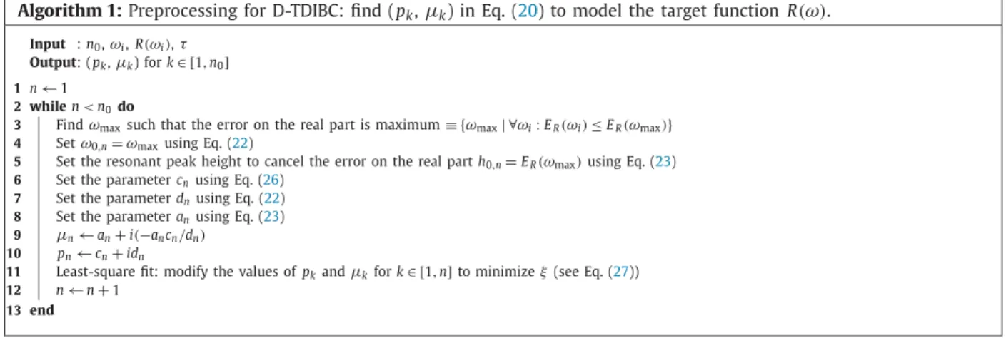
t is very smallso that the nonumerical stability issues were encountered by the authorswhile usingpolesandresiduesprovidedbyAlgorithm1.

Algorithm 1: PreprocessingforD-TDIBC:find(pk,

µ

k)inEq. (20) tomodelthetargetfunctionR

(

ω

)

. Input : n0,ωi,R(ωi),τ

Output: (pk,µk)fork∈ [1,n0]

1 n_←1

2 while n<n0do

3 Findωmaxsuchthattheerrorontherealpartismaximum≡ {ωmax|∀ωi:ER(ωi)≤ER(ωmax)}

4 Setω0,n=ωmaxusingEq. (22)

5 Settheresonantpeakheighttocanceltheerrorontherealparth0,n=ER(ωmax)usingEq. (23)

6 SettheparametercnusingEq. (26)

7 SettheparameterdnusingEq. (22)

8 SettheparameteranusingEq. (23)

9 µn←an+i(−ancn/dn)

10 pn←cn+idn

11 Least-squarefit:modifythevaluesofpkandµkfork∈ [1,n]tominimizeξ(seeEq. (27))

12 n←n+1

13 end

4. Validationforpurelyreflectivetime-delayedimpedance

Section3hasprovidedthemodelingmethodologynecessarytoaccountforacousticdelays.Inthissection,theobjective istwofold:(1)todemonstratetheapplicabilityofthemodelingprocedureonalimitcase:thedelayedpurereflection,(2) to validatetheabilityofTDIBC toimposea timedelay toaccountforacousticwave propagationinthetruncatedportionof thedomain.InSec.4.1wepresenttheone-dimensionalnumericalsetupusedforvalidation.Themethodologyproposedin Sec.3willbeusedtomodelareflectioncoefficientcorrespondingtoapuredelay.InSec.4.3atime domainsimulationis usedtodemonstratethatD-TDIBCimposesthecorrecttimedelay

τ

,waveamplitudeandphase.

4.1. Testcasepresentation

The aim of the simulation is to study the propagation of a Gaussian acoustic wave in the domain

Ä

defined on

x

_{∈ [−}

1

,

1

.

75

_]

m (Fig.6(a)).Themeanspeedofsoundisc0

=

350 m s−1.Thisperturbationwillpropagateonthepositivex

direction.Thephysicaldomainissplitintotwosub-domains:

Ä

_{= Ä}

c

+ Ä

m.Thecomputationaldomain

Ä

c isx

∈ [−

1

,

1

]

m

andthemodeleddomain

Ä

m isx

∈ [

1

,

1

.

75

]

m (grayareainFig. 6(a)). TheD-TDIBC isusedto modelthewave

propaga-tionin

Ä

m.Atthe leftboundary condition (x

=

xl

= −

1 m)thereflectioncoefficient is Rl

=

1 and attherightboundary

condition(x

₌

xr

=

1

.

75 m)thereflectioncoefficientis Rr

= −

1.Inthecomputationaldomain,thereflectioncoefficientat

x

₌

1 m accountingfor Rr hastobe modeled bya timedelay (see Sec.1) leading to Rr

|

x₌1 m

= −

e−iωτ .The time delay

correspondingtothismodeleddomainis

τ

₌

2

(

xr

−

xBC

)/

c0

=

4

.

28 ms.Theacoustictimefortheinitialwavelocatedinx0

totravelbackatitsinitialpositionisT

₌

2

(

xr

−

x0

)/

c0

=

10

.

0 ms. 4.2.Delayedimpedancemodeling

Toimposeapure time delay,theD-TDIBCmethodfirst requirestobuild amodelforthedelayedreflectioncoefficient usingtheAlgorithm1(seeSec.3). Intheory,thedelayedreflectioncoefficient Rr

|

x=1 m

= −

e−iωτ mustbemodeled upto

infinitefrequencies.Inpractice,itisnotfeasibleasitwouldrequireaninfinitenumberofPBFs.Innumerousapplications, thefrequencies of interest are limitedto agiven range(Fig. 6(b)) andit is sufficientto model R

(

ω

)

below acutoff fre-quency fc.For f

>

fc,anon-reflecting boundarycondition isused.Forexample,forthesetup presentedinFig.6(a),the

frequencycontentoftheinitialGaussianwaveisbelow1 kHz sothatthechosencutofffrequencyis fc

=

1 kHz.Alow-pass

filterisappliedtothetheoreticaldelayedreflectionbymultiplyingthedelayedreflectioncoefficientbyanenvelopefunction

ψ

allowingasmoothtransitionfrom1to0overafrequencyrange:

ψ (

f

)

₌

1 2

·

1

₋

tanh

µ

_f

−

fc

δ

¶¸

(30)

where f isthefrequencyand

δ

isaconstantthatspecifiesthefrequencyrangeofthetransitionfrom1to0(seeFig.6(b)). Theenvelopfunction

ψ

keepsthephaseofthedelayedreflectioncoefficientunchanged.Thetargetfunctiontobemodeled isthen:

R

(

ω

)

_{= ψ(}

f

)

_×

Rr

|

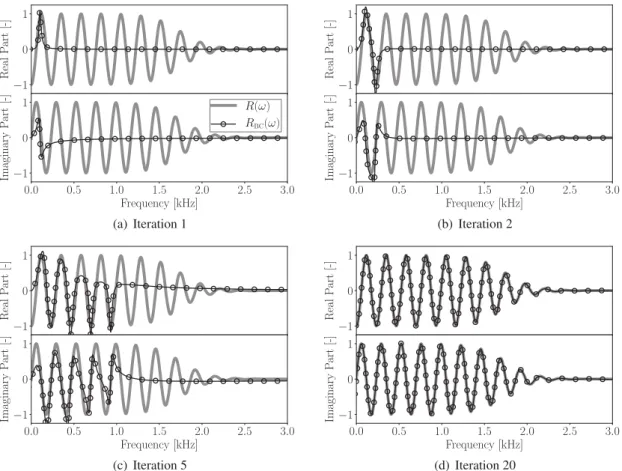
x₌1m (31)

Fig.7showsthemodelatiterations1,2,5and20oftheIterativeMulti-PoleModelingTechnique(Algorithm1). R

(

ω

)

is thefiltereddelayedreflectioncoefficientshowninFig.6(b)andRBC

ω

)

isthereflectioncoefficientmodelatagiveniteration definedinEq. (13).Theirrealandimaginarypartsareshowninthe topandbottomplots,respectively.At eachiteration,

Fig. 6. (a)Initialsolutionandvisualizationofthecomputational(Äc)andmodeled(Äm)domains.(b)Theoretical(graysolidline)andfiltered(blacksolid

line)delayedreflectioncoefficients.Thefiltershape(Eq. (30))isshown(blackdashedline).

Fig. 7. ReflectioncoefficientRBC(ω)modeledbytheIterativeMulti-PoleModelingTechniquealgorithm(Algorithm1inSec.3.3)aseveraliterations.An

accuratemodelisobtainedforn0=20,wheren0isthenumberofPBFRkasinEq. (20).

themethodfindsthebiggestpoint-to-pointorienteddistancebetweentherealparts(Eq. (28))ofR

(

ω

)

andRBC

ω

)

.Fig.7(a)

showsthemodelattheendofthefirstiteration.TheinitialsolutionofRBC

(

ω

)

targetsthefirstpeakintherealpartwhere

ℜ(

R

(

ω

))

=

1.In Fig. 7(b),the targetedpeak is where

_ℜ(

R

(

ω

))

= −

1. At an iteration i, initial guesses for pi and

µ

i are

found to targeta single peak atthetime. Fig. 7illustrates howthe modelpropagatesfromlow to highfrequencies.The algorithm isconsidered convergedafter 20iterations asthe maximumpoint-to-point erroronthe modulus isbelow1%, wherewedefinetheerrorasE

₌

max

(

_|

R

(

ω

)

₋

RBC

(

ω

,

n0

=

20

)

|)

.TheD-TDIBCmodelusedhereis,thus,madeof20poles

andresidues(pk,

µ

k),thatistosayonly40complexconstants(cf. AppendixA).

At

ω

₌

0,themodulusofthereflectioncoefficienttobemodeledis

_|

R

(

ω

=

0

)

|

=

1.Suchaconditioncannotbefulfilled bytheD-TDIBCaseachofthePBFhasanullmodulusatthezero-frequencylimit:

_|

Rk

(

ω

=

0

)

|

=

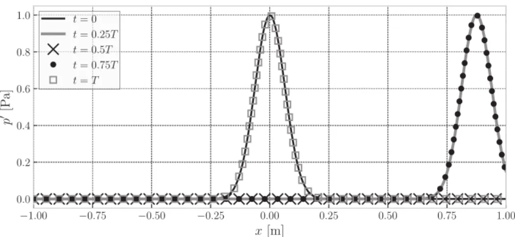
0.However,thefrequency

Fig. 8. PropagationandreflectionofaGaussianpressurewaveinthedomainÄc+ ÄmbysimulatingonlyÄc.TheacousticpropertiesofÄmareimposed

usingD-TDIBC.

atwhichthemodulus ofthereflectioncoefficient modeled byD-TDIBC becomes zerocanbe madearbitrarily low inthe fittingstage.Themodulusofthemodeledreflectioncoefficient RBC

(

ω

)

,presentedinFig.7(d),tendstozeroforfrequencies

below0

.

1 Hz.

Thereflectioncoefficientmodeled bythepolesandresiduesfulfillsthecausalityandreality conditionsby construction ofthemethod.However, itisinterestingtonote thatforasmallnumberofpolesandresidues(hencefora lowaccuracy ofthefit) thepassivity condition isviolated,asshowninFig. 7(a) where

_|

R

(

ω

)

_|

>

1 around0.15 kHz. Nonetheless,fora highernumberofpolesandresidues,thepassivityconditionisalsoverified.

4.3.One-dimensionalwavepropagation

Inthissection,thebehavioroftheD-TDIBCisinvestigatedfirstonabasicone-dimensionalwavepropagationproblem. ThenthetimedomainresponseofeachPBFisinspectedtohighlightthemechanismofD-TDIBC.

Theone-dimensionalwavepropagationiscomputedusingtheAVBPsolver.AVBPisathree-dimensionalfully compress-ible Navier–Stokesequation solver. Atwo-step Taylor–Galerkin scheme,calledTTGCis used.TTGC isthird-orderaccurate inspaceandtime [41,42]. Characteristicsboundary conditions(NSCBC)areused [5,8,43,44].Inthe NSCBCframeworkthe characteristicwavesare evaluated atthe boundaries. TDIBC prescribes theingoing characteristic wave fromtheoutgoing characteristicwaveandis,thus,consistentwiththeNSCBCformalism.

Asthereflectioncoefficientmodeledinxr isRr

= −

1,thewaveisa priori expectedtobefullyreflected:theamplitude

ofthereflectedwavemustbeequaltotheoneoftheincidentwave.As Rrisreal-valued,thereflectedwaveisexpectedto

becenteredinx

₌

0 m afteratimet

₌

T (seeSec.4.1).

Fig.8illustratesthepropagationofthepressurewavefromtimet

₌

0 uptot

₌

T .Att

₌

0 thepressurefieldcorresponds totheinitialsolutionshowninFig.6(a).Att

₌

0

.

25T thewavehaspropagatedinthepositive x directionandiscrossing theboundaryconditionatx

₌

xBC

=

1 m.Att

=

0

.

5T thepressurewavehascompletelyleftthecomputationaldomain.This

resultisexpected:attimet

₌

0

.

5T thewaveispropagatinginsidethemodeleddomain

Ä

m,i.e.thetruncatedportion(gray

areainFig.6(a)).Ifonewereto computethecompletedomain,att

₌

0

.

5T theacousticpressure p′

(

x

)

wouldbe zerofor

x

_{∈ [−}

1

,

1

_]

m.Att

₌

0

.

75T thepressurewave isre-injectedinthecomputationaldomainbytheboundarycondition. The reflectedpressurewavehasthesameamplitudethantheincidentwave(1 Pa)asexpected. Att

₌

T thereflectedGaussian waveiscenteredatx

₌

0 m whichmeansthatthetimedelayispreciselyprescribedbyD-TDIBC.

The acousticpressure and velocity atthe boundary are recorded atthe boundary condition at xBC

=

1 m during the

simulation.TheresultsareshowninFig.9(a).Additionally,theacousticenergy Ea containedinthedomainisshown.For

thesakeofclarity,eachvariableisnormalizedbyitsmaximum.Atfirstnoacousticactivityisseenasthewavepropagates insidethedomain,theacousticenergyismaximum.

Theacousticpressurep′attheboundaryinFig.9(a)isconsistentwiththeresultsinFig.8.Atfirstnoacousticpressure isseenbytheboundaryuntil theGaussianwave crossestheboundaryatt

_≃

0

.

25T

_≃

2

.

5 ms. Afterthewave hascrossed theboundary,theacousticpressure returnstozero.Afterthe timedelay

τ

(Fig. 9(a))att

_≃

0

.

75T

_≃

7

.

5 ms thereflected waveisre-enteringthecomputationaldomainwiththesameamplitudeastheincidentwave.Finally,theacousticpressure

p′returnstozero.Theamplitudeofthereflectedacousticvelocityu′(t

_≃

0

.

75T

_≃

7

.

5 ms)isalsothesameastheincident wave (t

_≃

0

.

25T

_≃

2

.

5 ms) although thesign is changed: u′ isnegative. Thisindicates that the wave is travelingin the negativex directionafterthereflectionatxr

=

1

.

75 m.Thisresultisconsistentwiththeimpositionofareflectioncoefficient

Rr

= −

1 inxr.Whenthewavecrossestheboundarytheacousticenergyinitiallycontainedinthedomainislostduetothe

Fig. 9. (a)Acousticvelocity(dashedline)andpressure(solidlinewithcircles)attheboundarycondition.(b)Temporalresponseof20PBF(dashedand dottedlines)andoftheingoingwaveimposedbytheD-TDIBC(blacksolidline).

thereflectedwave re-entersthedomain.Thisstressesthefactthat D-TDIBCconservestheacousticenergywhileimposing atimedelay.

In their work, Jaensch et al. [14] solve a similar problem: they impose a pure time delay at a boundary condition withaone-dimensionalincident Gaussianwave.AsdiscussedinSec. 1,theirmethodusesafirstorderupwindnumerical scheme to discretize the one-dimensional LEE over the truncated domain. Their method is, thus, inherently dissipative andthedissipationincreaseslinearlywiththecellsizeofthespatial discretization.Inordertoachieve adissipationlevel comparabletotheoneobtainedhere,itwasnecessarytouse1000points.Asaconsequence,inthestate-spacemodelused, thestatematrixisofdimension2000

_×

2000,i.e.4millionscalarvalues.D-TDIBCseemstoyieldcomparableresultsfora lowermemorystoragerequirementasonly40complexconstantswereusedtomodelthedelayedreflectioncoefficient.

Fig.9(b)illustratesthecontributionofeachPBFRk.TheingoingwaveAinn

(

t

)

imposedbyD-TDIBCisthesumofallthe Rk.

Before t

_≃

7 ms theingoing waveisnull:thePBFs arecanceling eachother out.Att

_≃

7 ms theindividualcontributions ofthePBFsstopcancelingthemselvesout:theyadduptocreatethere-enteringcharacteristicwave.Thisstresseshowthe modelingprocedureofR

(

ω

)

iscriticalforanaccuratepredictionofacousticdelays.

5. Validationforacombustionchamber

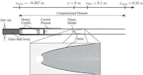
Inthissection, weinvestigatethethermoacousticinstability [45] inalaminarexperimentalsetupcalledINTRIGBurner (IMFT,Toulouse).First,aDNSofthefullsetup(called“FULL”)isconducted.AsecondDNS(called“TRUNCATED”)inwhich thecomputationaldomainistruncatedaftertheflameisconducted.IntheTRUNCATEDcase,D-TDIBCisusedtomodelthe acousticpropertiesofthetruncateddomainasinSec.4.TheresultsobtainedusingD-TDIBCwillbecomparedwiththose oftheFULLconfiguration.

5.1. Experimentalsetup

The INTRIGBurnerisusedtostudyalean premixedlaminarmethane–airflame attachedon acylinder.The operating pointcorrespondstoanequivalenceratio

φ

₌

0

.

75 andabulkvelocityofthefreshgasesofub

=

0

.

8 m s−1.Theassociated

laminarflamespeedandadiabatictemperaturearesl

=

0

.

23 m s−1 andTad

=

1920 K.

The experimental rig is shownin Fig.10. The gaseous methane–air premixture isinjected upstream of the glassball arraylocatedatx

_{= −}

0

.

367 m.Theflowisthenlaminarizedbytheglassballsandthehoneycombpanels.Aleanpremixed methane–air laminar flamethen attachesto a cylindricalstainless-steel flameholder ofwith adiameter d

₌

8 mm.The combustionchamberhasaconstantcrosssectionofh

₌

34 mm byl

₌

94 mm.

5.2. Numericalsetup

As the flow is two-dimensional, 2D Direct Numerical Simulation (DNS) approach can be used [46–48]. A 19-species mechanism (calledLU19) isused [49] forthe modeling ofchemical kinetics.Schmidt and Prandtlnumbers are assumed constant: Pr

₌

0

.

6 and Sc

₌

0

.

6. The full meshis composed of625 000cells. The reduced meshis composed of545 000 cells,i.e.areductionof13%.Theflamethicknessis

δ

0_L

₌

680 µm andatleast11points areusedtoresolvetheflamefront withameshresolutionattheflameof

1

x

₌

60 µm [46–48].Atypicalflame,hereatastableoperatingpoint,isshownin Fig.10(bottom).

Theinletacousticboundary(glassballsatx

_{= −}

0

.

367 m) isa hardwall(i.e.u

(

ω

)

₌

0 m s−1 _{atallfrequencies).Itwas}

checkedintheexperimentthatthisisagoodapproximation [48].Thisassumptionisclosetorealisticconditionsastheinlet BCcorrespondstotheglassballsarray.Theoutletacousticboundary(atx

₌

0

.

35 m)isanopen-end(i.e. p

(

ω

)

=

0 Pa atall frequencies).Thisissueshouldbetakencareofifonewerewillingtocomputeaccuratelythethermoacousticstabilityofthe

Fig. 10. SketchofatransversecutoftheINTRIGBurner(top).ThecomputationaldomainoftheFULLconfigurationgoesfromtheglassballsarray(x= −0.367 m)totheexhaust(x=0.35 m)whileitiscut(atx₌xBC=0.1 m)intheTRUNCATEDconfiguration.Azoom(bottom)oftheflameregionof theinitialsolutionusedinDNSisshown.ThelightgreyanddarkgreyregionsrepresentthezeroandhighCO2massfractionlevels.Thestreamlinesare

plottedinwhite.

Fig. 11. Schematic of the computational domains and BC used for the two simulations: FULL and TRUNCATED cases.

Table 1

Parametersusedinthetwosimulations.

Case Domain length Ncell 1xmin Inlet BC Outlet BC Outlet BC method

FULL 0.717 m 625000 60 µm R(ω)= −1 RFULL(ω)=1 NSCBC

TRUNCATED 0.467 m 545000 60 µm R(ω)_{= −}1 RTRUNCATED(ω)=e−iωτ D-TDIBC

configuration.However,thegoalofthispaperismoremodest:itaimstovalidate D-TDIBC.Thesimpleacousticconditions usedherearethusacceptableasthereferencecaseisanumericalsimulation.

Twosimulations arecarriedout andinvestigatedinthissection(Fig. 11):the “FULL”andthe“TRUNCATED”cases.The outlet boundary condition of the FULL domain is located as x

₌

0

.

35 m and the outletD-TDIBC boundary condition of the TRUNCATEDdomain is located at x

₌

0

.

1 m. Fig. 11 showsthe computational domain andthe boundary conditions usedinthethreesimulations.Thegreyarea intheTRUNCATEDcasecorresponds tothedomainwheretheacousticwave propagationismodeledbyatimedelayimposedbyD-TDIBC.Table1summarizestheparametersusedinthesimulation.

ThetruncationofthegraydomaininFig.11ispossibleastheflowisstronglyone-dimensionalandhomogeneous.For instance,the axial velocity is 4 orders ofmagnitude higherthan the maximum ofthe vertical velocity in the truncated portion.

5.3.D-TDIBC:reflectioncoefficientmodel

The Iterative Multi-Pole Modeling Technique presented in Sec. 3 is used to model the acoustic wave propagation in the truncatedpartof the INTRIGBurner. The outletboundary conditions ofthe Full andTruncated domains are located at xmax

=

0

.

35 m and xBC

=

0

.

10 m, respectively. Consequently, the length of the domainto be modeled by D-TDIBC is

L

₌

0

.

25 m.The value ofxBC must belarge enoughto ensurethat combustioniscomplete andonly acousticstake place

betweenxBC and xmax. Moreover, the soundspeed must be homogeneous in thiszone. This condition hasbeen verified a posteriori byanalyzingtheresultsofthe FULLconfigurationsimulation: thesoundspeedfluctuationsare lessthan 0.5% ofthemeanvalue c0

=

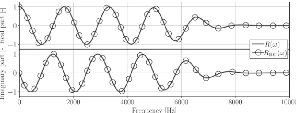
830 m s.Accordingtoduct acousticstheory,plane wavespropagatesinductsatfrequencies lower

thatacutofffrequency fc [34].Thisfrequencyisgivenbythespeedofsoundc0andthelowestheightinthecrosssection.

In theINTRIG setup, the plane wavespropagate at frequencies lower that fc

=

3

.

5 kHz. The filteringprocedure used in

(Sec.4.2)isappliedheresothatthefrequencieslowerthan fc

=

3

.

5 kHz areaccuratelymodeled.Theresultsareshownin

Fig.12.Thereflectioncoefficientmodelusedhereconsistsinasetof18(pk,

µ

k)andverifiescausality,realityandpassivity

Fig. 12. ModelofthedelayedreflectioncoefficientRBC(ω)withn0=18 (seeEq. (13))foratime-delayofτ=0.30 ms inthelaminarcombustorofFig.10.

Fig. 13. (a)SpectraobtainedfortheFULLandtheTRUNCATEDsimulations.D-TDIBCallowsanaccuratepredictionofthethermoacousticstabilityobserved intheFULLconfiguration.Thespectraarebasedonaprobelocatedatx= −8.5 mm.Theshapesofthefirst(b),second(c)andthird(d)modescorrespond totheacousticeigenmodesofaleft-handsideclosedandright-handsideopenductmodifiedbythejumpofcharacteristicimpedancebetweenthefresh andburntgases.Themarkerscorrespondtotheprobesinthesimulation(linesareaddedforthesakeofclarity).

5.4. Resultsanddiscussion

Theflow setupinFig.10isthermoacousticallyunstable:theflameoscillatesandcouplestotheacousticmodesofthe setup [45].TheinstabilityissustainedinDNSoftheFULLandTRUNCATEDconfigurations(Fig.11).Fig.13(a)illustratesthe

SoundPressureLevel(SPL)spectraexpressedindB anddefinedasSPL

₌

20log

(

p

/

pref

)

basedonareferencepressurelevelof pref

=

2

·

10−5Pa.TheFULLsimulation,i.e.computingthefulldomain,showsastrongacousticactivitywithmanyamplified

acousticmodes.Fourprinciplemodesarefound,withfrequencies203 Hz,534 Hz,782 Hz and1150 Hz, respectively.The modeshapescanbe obtainedby(1)performing a spectralanalysisatseveralaxiallocationsoftheburner,(2)extracting theamplitudeoftheFouriertransformatthepeakfrequencyinFig.13(a)and(3)normalizingbythemaximumpressure amplitude. The three firstmodes observedin the FULLsimulation area quarter wave mode (Fig. 13(b)), a three-quarter wavemode(Fig.13(c))andafive-quarterwavemode(Fig.13(d)).

TheTRUNCATEDsimulationalsoexhibitsthermoacousticinstabilitiesandisingoodagreementwiththeFULLsimulation. Fig.13(a)illustratestheabilityofD-TDIBCtoaccuratelypredictthebroadbandacousticactivity,despitetheclearnonlinear excitationofhigherharmonics,duetothehighpressureamplitudeslevels.Inparticular,theagreementbetweenvaluesof theexcitedfrequencies(Fig.13(a))andthemodeshapes(Figs.13(b), (c) and (d))isremarkable.

SomediscrepanciesarevisibleinthemagnitudeoftheSPLspectrum,wheretheTRUNCATEDsimulationsoverall under-predicttheintensityoftheSPLs.Thisdiscrepancycanbeattributedtotwoconcurrentissues.First,thereflectioncoefficient usedattheoutletoftheFULLsimulation is

_|

RFULL

|

=

1 forallfrequencies, whilethisis trueonlyinaselectedfrequency

rangeofinterest(dueto thefilteringprocedureused,cf. Fig.12andFig.6(b)) fortheTRUNCATEDsimulation.Outsideof that range,themagnitudeof thereflectioncoefficient drops below 1,hence causingspurious acousticenergyloss atthe D-TDIBCboundary.Second,thelargeamplitudeofthepressureoscillationsatthelimitcyclemaytriggerlossesdueto non-linearacousticeffectswhicharedirectlysimulatedintheFULLsimulationsinaportionofthedomainthatisnotpresent intheTRUNCATEDsimulations.

Overall,Fig. 13demonstrates that D-TDIBCcan satisfactorily recoverthe acousticeigenmodes ofa domainwhile sim-ulatingonlyapartofit. Italsogivestheopportunity toinvestigatethethermoacousticstability ofdifferentsetupswhile simulatingthesamecomputationaldomain:thelengthofthetruncateddomaincanbeadjustedwithinthesameDNS sim-plybyintroducingadifferenttimedelayattheboundaryx

₌

xBC(Fig.10),withouttheneedtocreateanewcomputational

mesh.

6. Conclusion

A novel numerical strategy calledDelayed-Time Domain Impedance Boundary Condition (D-TDIBC) has been derived fromanexistingTDIBCapproach [1–4] inordertoaccountfortimedelaysinNavier–Stokessimulation.Themethodallows tomimic acousticwave propagationin domains largerthan thecomputational domain usedin thenumericalstudy. The benefits are twofold: (1) computational cost can be saved andspatial resolution can focus on areas ofinterest, (2) any additionallengthcan beaddedtothe computationaldomainallowing straightforwardinvestigations ofgeometrychanges downstreamorupstreamofthezoneofinterest.Whiletheformermainlyconcernsstructuredmeshes,thelatterappliesto alltypesofgrids.

D-TDIBCisanextensionofTimeDomainImpedanceBoundaryCondition(TDIBC)methods [1–4].Theproposed methodol-ogyworkswiththereflectioncoefficientR

(

ω

)

andgivesaccuratemodelsfortimedelayedfullyreflectingacousticboundary conditionssuchasclosedandopen-endconditions.Thesemodelswereusedinthetimedomainsimulationsandwerefound togiveaccurateacousticwavepropagationpropertiesforbothone-dimensionalandtwo-dimensionalreactiveNavier–Stokes simulations.

Theone-dimensionalwavepropagationresultsillustratethecapacityofD-TDIBCtoaccuratelyimposeatimedelaywhile conservingtheacousticenergyincaseofafullreflection.TheinvestigationonindividualPoleBaseFunctions(PBFs)stresses theneedforanaccuratemodelingstrategy.Indeed,thetimedelayedresponseoftheboundaryresultsinacancellationof individualresponses:thePBFs.Thisisaccomplishedthroughthediversityoftheiramplitudes,pseudo-periodsandphases.

Thetwo-dimensionalsimulationfocusesonthethermoacousticstabilityofalaminarcombustionchamber (theINTRIG Burner [46–48])withalean premixedlaminarmethane–airflameattachedon acylinder.Aportion oftheoutletdomain was truncatedandtheacoustic wave propagationwas modeled withD-TDIBC.The D-TDIBC simulationwas compared to a reference simulation where the full domain is taken into account. D-TDIBC was found to give accurate predictions of the thermoacousticstability while saving computational resources. The frequencies, amplitudes andmode shapes are in excellentagreementwiththereferencesimulation.

Acknowledgements

The research leading to theseresults has received funding fromthe European Research Council underthe European Union’sSeventhFrameworkProgramme(FP/2007–2013)/ERCGrantAgreementERC-AdG319067-INTECOCIS.Thisworkwas grantedaccesstothe high-performancecomputingresourcesofCINESundertheallocation A0012B07036madebyGrand EquipementNationaldeCalculIntensif.ThesupportofCalmipforaccesstothecomputationalresourcesofEOSis acknowl-edged.

CarloScaloacknowledges the support ofPurdue’s RosenCenter forAdvanced Computing (RCAC),the Air Force Office ofScientific Research (AFOSR) grants FA9550-16-1-0209 (Core Program) andFA9550-18-1-0292 (2018 Young Investigator Program),andNSF’sFluidsDynamicsProgram(Award#1706474).

Appendix A. D-TDIBCmodel:1Dwavepropagationproblem(TableA.2)

Table A.2

Polesandresiduesusedintheone-dimensionalpuredelayedGaussianwavepropagationproblem.

Rk ak bk ck dk ω0,k[rad s−1] f0[Hz]

k=1 4.91e+05 4.56e+05 −3.23e+03 3.48e+03 4.75e+03 7.56e+02

k=2 −1.10e+04 −7.38e+03 −9.52e+02 1.42e+03 1.71e+03 2.72e+02

k=3 −8.21e+04 −3.92e+04 −1.38e+03 2.89e+03 3.20e+03 5.09e+02

k₌4 −1.33e+05 −4.66e+04 −1.50e+03 4.29e+03 4.54e+03 7.23e+02

k₌5 ₋6.17e₊04 ₋1.39e₊04 ₋1.30e₊03 5.79e₊03 5.93e₊03 9.44e₊02

k₌6 ₋3.22e₊04 ₋5.12e₊03 ₋1.15e₊03 7.26e₊03 7.35e₊03 1.17e₊03

k=7 −1.73e+04 −2.04e+03 −1.03e+03 8.73e+03 8.79e+03 1.40e+03

k=8 −1.19e+02 2.65e+07 −2.17e+02 −9.77e−04 2.17e+02 3.46e+01

k=9 −2.11e+00 6.77e+04 −1.89e+00 −5.88e−05 1.89e+00 3.01e−01

k₌10 −9.15e+03 −8.40e+02 −9.34e+02 1.02e+04 1.02e+04 1.63e+03

k₌11 −1.32e+05 −1.15e+05 −7.95e+03 9.11e+03 1.21e+04 1.92e+03

k₌12 6.55e₊02 5.49e₊02 ₋5.20e₊02 6.20e₊02 8.09e₊02 1.29e₊02

k=13 −5.04e+03 −4.09e+02 −9.40e+02 1.16e+04 1.16e+04 1.85e+03

k=14 −2.25e+03 −1.70e+02 −9.78e+02 1.30e+04 1.30e+04 2.07e+03

k=15 −3.80e+01 −8.77e+07 −7.84e+01 3.40e−05 7.84e+01 1.25e+01

k=16 −7.67e+03 −9.34e+02 −1.80e+03 1.48e+04 1.49e+04 2.37e+03

k₌17 6.89e+00 1.17e−01 −1.61e+02 9.46e+03 9.46e+03 1.51e+03

k₌18 −1.50e+01 1.75e+06 −2.93e+01 −2.51e−04 2.93e+01 4.67e+00

k₌19 3.82e₊03 3.80e₊02 ₋1.50e₊03 1.50e₊04 1.51e₊04 2.40e₊03

k=20 −6.06e+00 −7.54e+05 −9.40e+00 7.56e−05 9.40e+00 1.50e+00

Appendix B. D-TDIBCmodel:2DreactiveDNSoftheINTRIGBurner(TableB.3)

Table B.3

Polesandresiduesusedinthetwo-dimensionalreactiveDNSoftheINTRIGBurner.

Rk ak bk ck dk ω0,k[rad s−1] f0[Hz]

k=1 1.91e+05 −5.06e+04 −8.06e+03 −3.04e+04 3.14e+04 5.00e+03

k=2 −3.24e+06 −1.10e+07 −1.83e+04 5.39e+03 1.91e+04 3.04e+03

k=3 1.47e+06 1.97e+06 −1.17e+04 8.74e+03 1.46e+04 2.32e+03

k=4 5.20e+05 2.55e+05 −9.61e+03 1.96e+04 2.18e+04 3.47e+03

k₌5 1.33e+03 −3.60e+09 −2.74e+03 −1.01e−03 2.74e+03 4.37e+02

k₌6 5.06e+02 −1.41e+09 −1.06e+03 −3.81e−04 1.06e+03 1.69e+02

k₌7 7.45e₊05 1.08e₊06 ₋3.97e₊04 2.75e₊04 4.83e₊04 7.69e₊03

k=8 −2.45e+03 −2.62e+02 −3.78e+03 3.54e+04 3.56e+04 5.66e+03

k=9 3.15e+04 4.45e+03 −5.68e+03 4.02e+04 4.06e+04 6.46e+03

k=10 6.28e−03 −1.01e+05 −6.28e−03 −3.93e−10 6.28e−03 1.00e−03

k=11 2.16e+02 −3.31e+07 −3.85e+02 −2.51e−03 3.85e+02 6.13e+01

k₌12 1.86e+01 2.39e−03 −1.08e−02 8.46e+01 8.46e+01 1.35e+01

k₌13 7.04e₋01 3.79e₋14 ₋4.51e₋12 8.38e₊01 8.38e₊01 1.33e₊01

k₌14 5.11e₊03 6.29e₊02 ₋6.01e₊03 4.88e₊04 4.92e₊04 7.83e₊03

k=15 2.66e+05 1.33e+05 −2.10e+04 4.20e+04 4.70e+04 7.47e+03

k=16 1.89e+01 2.85e+05 −6.39e+01 4.24e−03 6.39e+01 1.02e+01

k=17 6.76e+03 1.68e+03 −5.56e+03 2.23e+04 2.30e+04 3.66e+03

k=18 5.92e+01 −6.50e+01 −1.14e+02 −1.04e+02 1.54e+02 2.45e+01

References

[1]K.Y.Fung,H.B.Ju,Broadbandtime-domainimpedancemodels,AIAAJ.39 (8)(2001)1449–1454.

[2]K.-Y.Fung,HongbinJu,Time-domainimpedanceboundaryconditionsforcomputationalacousticsandaeroacoustics,Int.J.Comput.FluidDyn.18 (6) (2004)503–511.

[3]CarloScalo,JulienBodart,SanjivaK.Lele,Compressibleturbulentchannelflowwithimpedanceboundaryconditions,Phys.Fluids27 (3)(2015)035107.

[4]JeffreyLin,CarloScalo,LambertusHesselink,High-fidelitysimulationofastanding-wavethermoacoustic–piezoelectricengine,J.FluidMech.808(2016) 19–60.

[5]T.Poinsot,S.Lele,Boundaryconditionsfordirectsimulationsofcompressibleviscousflows,J.Comput.Phys.101 (1)(1992)104–129.

[6]WolfgangPolifke,CliftonWall,ParvizMoin,Partiallyreflectingandnon-reflectingboundaryconditionsforsimulationofcompressibleviscousflow,J. Comput.Phys.213 (1)(2006)437–449.

[7]T.Poinsot,D.Veynante,TheoreticalandNumericalCombustion,thirdedition,2011.

[8]G.Lodato,P.Domingo,L.Vervisch,Three-dimensionalboundaryconditionsfordirectandlarge-eddysimulationofcompressibleviscousflow,J.Comput. Phys.227 (10)(2008)5105–5143.