HAL Id: hal-00328304
https://hal.archives-ouvertes.fr/hal-00328304v2
Submitted on 20 May 2019
HAL is a multi-disciplinary open access
archive for the deposit and dissemination of
sci-entific research documents, whether they are
pub-lished or not. The documents may come from
teaching and research institutions in France or
abroad, or from public or private research centers.
L’archive ouverte pluridisciplinaire HAL, est
destinée au dépôt et à la diffusion de documents
scientifiques de niveau recherche, publiés ou non,
émanant des établissements d’enseignement et de
recherche français ou étrangers, des laboratoires
publics ou privés.
Sea surface wind speed estimation from space-based
lidar measurements
Y. Hu, K. Stamnes, M. Vaughan, Jacques Pelon, C. Weimer, D. Wu, M.
Cisewski, W. Sun, P. Yang, B. Lin, et al.
To cite this version:
Y. Hu, K. Stamnes, M. Vaughan, Jacques Pelon, C. Weimer, et al.. Sea surface wind speed estimation
from space-based lidar measurements. Atmospheric Chemistry and Physics, European Geosciences
Union, 2008, 8, pp.3593-3601. �hal-00328304v2�
www.atmos-chem-phys.net/8/3593/2008/ © Author(s) 2008. This work is distributed under the Creative Commons Attribution 3.0 License.
Chemistry
and Physics
Sea surface wind speed estimation from space-based lidar
measurements
Y. Hu1, K. Stamnes2, M. Vaughan1, J. Pelon3, C. Weimer4, D. Wu5, M. Cisewski1, W. Sun1, P. Yang6, B. Lin1, A. Omar1, D. Flittner1, C. Hostetler1, C. Trepte1, D. Winker1, G. Gibson1, and M. Santa-Maria1
1Climate Science Branch, NASA Langley Research Center, Hampton, VA, USA 2Dept. of Physics and Enginerring, Stevens Institute of Tech., Hoboken, NJ ,USA 3Universit´e Pierre et Marie Curie, Service d’Aeronomie/IPSL, Paris, France 4Ball Aerospace & Technologies Corp., Boulder, CO, USA
5The Key Laboratory of Ocean Remote Sensing, Ocean University of China, Qingdao, China
6Dept. of Atmospheric Sciences, Texas A.& M. University, College Station Commerce Street,TX, USA
Received: 3 January 2008 – Published in Atmos. Chem. Phys. Discuss.: 12 February 2008 Revised: 7 May 2008 – Accepted: – Published: 8 July 2008
Abstract. Global satellite observations of lidar backscatter
measurements acquired by the Cloud-Aerosol Lidar and In-frared Pathfinder Satellite Observation (CALIPSO) mission and collocated sea surface wind speed data from the Ad-vanced Microwave Scanning Radiometer for the Earth Ob-serving System (AMSR-E), are used to investigate the rela-tion between wind driven wave slope variance and sea sur-face wind speed. The new slope variance – wind speed tion established from this study is similar to the linear rela-tion from Cox-Munk (1954) and the log-linear relarela-tion from Wu (1990) for wind speed larger than 7 m/s and 13.3 m/s, re-spectively. For wind speed less than 7 m/s, the slope variance is proportional to the square root of the wind speed, assum-ing a two dimensional isotropic Gaussian wave slope distri-bution. This slope variance – wind speed relation becomes linear if a one dimensional Gaussian wave slope distribution and linear slope variance – wind speed relation are assumed. Contributions from whitecaps and subsurface backscattering are effectively removed by using 532 nm lidar depolarization measurements. This new slope variance – wind speed rela-tion is used to derive sea surface wind speed from CALIPSO single shot lidar measurements (70 m spot size), after correct-ing for atmospheric attenuation. The CALIPSO wind speed result agrees with the collocated AMSR-E wind speed, with 1.2 m/s rms error. Ocean surface with lowest atmospheric loading and moderate wind speed (7–9 m/s) is used as target for lidar calibration correction.
Correspondence to: Y. Hu
1 Introduction
It has been over half a century since Cox and Munk (1954) introduced the Gaussian distribution relation between sea surface wind and the slopes of wind driven waves. A Gaussian distribution has maximum information entropy [P P (si)logP (si), where P (si) is the probability of slope
si] and thus is the most probable state if we can consider the wind driven slopes (si) as many independent and identically-distributed random variables [central limit theorem]. In the same study, Cox and Munk (1954) also suggested a lin-ear relationship between wind speed (U ) at 12.5 m above sea surface and the variance (σ2) of the slope distribution [σ2(s)=aU +b, with a and b constants] based on mea-surements of the bi-directional sea surface reflectance pat-tern of reflected sunlight. Using laboratory measurements, Wu (1990) revised the relation between wind speed and slope variance to two log-linear relations. When the wind speed is less than 7 m/s, capillary waves, resulting from a balance be-tween atmospheric wind friction and water surface tension, is the predominant component of wind driven waves. For wind speed exceeding 7 m/s, the surface becomes rougher and the predominant wavelengths grow to centimeter scale while sur-face tension weakens and gravity becomes more important in terms of restoring surface smoothness (i.e., gravity-capillary waves). The wind speed U -wave slope variance σ2relation also varies with sea surface state and meteorological condi-tions (Shaw and Churnside, 1997).
Using collocated TRMM sea surface radar cross sec-tions and wind speeds from microwave radiometer, Freilich and Vanhoff (2003) analyzed the U −σ2-relations on a
3594 Y. Hu et al.: Sea surface wind speed estimation from space-based lidar
global scale and demonstrated that at lower wind speed (U <10 m/s), the log-linear relation agrees well with the ob-servations, while at larger wind speed (5 m/s<U <19 m/s), both the linear Cox-Munk relation and log-linear Wu rela-tion are within the uncertainty of observarela-tion.
The wave slope variances derived from microwave data are slightly different from those derived from visible and in-frared measurements since they cover different wave-number ranges of wind-generated waves (Liu et al., 2000). A global analysis of U −σ2-relations for waves that fall within the li-dar backscatter sensitivity range can be performed by com-paring sea surface backscatter of the CALIPSO lidar with the collocated wind speed measurements of AMSR-E on the Aqua spacecraft. As the space-based lidar onboard the CALIPSO satellite only measures sea surface backscatter at a 0.3◦off-nadir angle, directional properties, such as skewness and peakedness, can be ignored. The independent absolute calibration of CALIPSO lidar measurements enables an ac-curate assessment of the U −σ2-relations by comparing the AMSR-E wind speeds with the variance information derived from lidar backscatter.
The dependence of the lidar/radar backscatter cross sec-tion on the angle of incidence was proposed in theory by Barrick (1968), and verified qualitatively by measurements from airborne lidar (Bufton et al., 1983) and space-based li-dar (Menzies et al., 1998).
For a one dimensional Gaussian statistics, the wave slope distribution can be expressed as
q
1/(2π σX2)exp(−tan2θX
2σ2 X
), where tanθxis the wave slope along x direction and σx2is the
variance of the wave slope distribution.
A two dimensional wave slope distribution has a variance of σ2=σx2+σy2. The fraction F of a unit sea surface area covered by waves with wave slope tan θ =
q
tan2θ
x+tan2θy within an infinitely small incident solid angle δcosθ δϕ is (Genneken et al., 1998), F (θ, ϕ)dcos θ dϕ=tan θ 2π σ2exp(− tan2θ 2σ2 )dtan θ dϕ = 1 2π σ2cos3θexp(− tan2θ 2σ2 )dcos θ dϕ. (1)
where the integration of probability F over all slope (0≤tanθ ≤∞) and all azimuth (0≤ϕ≤2π ) for a unit sea sur-face area equals 1 (R0∞R02πF dtan θ dϕ=1).
For a lidar/ radar system pointing at off-nadir angle θL, the
specular reflection backscatters into the lidar receiver only if the wave slope tanθ equals tanθL. The incident area at sea
surface is the unit laser/receiver area divided by cosθ . Thus the cross section A(θ ) of lidar/radar backscatter at off-nadir incident θLis,
A(θ )dcos θ dϕ = ρ
2π σ2cos4θexp(−
tan2θ
2σ2 )dcos θ dϕ, (2)
where ρ is the Fresnel reflectance. For backscatter of lin-early polarized incident light, such as the laser beam
trans-mitted by CALIPSO, ρ=[(n-1)/(n+1)]2 at nadir incidence and at visible and near infrared wavelengths. The light re-flected from the surface is co-linearly polarized when the lidar backscatter contribution from multiple scattering be-tween waves is negligible. The lidar and radar backscatter cross section, ρ
2π σ2cos4θ exp(−
tan2θ
2σ2 )has a form similar to
Barrick’s (1968).
By definition, the sea surface backscatter cross section A is half of the integrated lidar backscatter γ (in the unit of sr−1)for opaque objects such as dense clouds and surfaces (Menzies, et al., 1998; Platt, 1973; Tratt et al., 2002), as
γ =R0∞Aexp(−2τ )dτ =A2. Here τ is the extinction optical depth along the line of sight. Thus, the CALIPSO lidar sea surface backscatter γ is,
γ = ρ
4π σ2cos4θ exp(−
tan2θ
2σ2 ) (3)
For near-normal incidence, ρ≈0.0209 for sea wa-ter at 532 nm and ρ≈0.0193 at 1064 nm. And exp[– tanθ2/(2σ2)]≈1, and cosθ ≈1. Thus, at 1064 nm,
σ2≈0.0193
4π γ (4)
Ideally, the lidar backscatter from sea surface comes from the surface range bin. Here the sea surface lidar backscatter is a sum of the surface bin plus one range bin above and 3 range bins below because of CALIOP’s low pass filter and detector transient response.
If a one dimensional Gaussian wave slope distribution is assumed, γ ≈√0.0193
8π σ2.
At near nadir incidence, for a two-dimensional Gaussian wave slope distribution, sea surface lidar backscatter is in-versely proportional to the variance. For a one dimensional Gaussian slope distribution, the lidar backscatter is inversely proportional to the square root of variance.
The two commonly referenced relations between wave slope variance and sea surface wind speed in the literature are,
– Cox and Munk (1954): σ2≈0.003+0.00512 U ;
– Wu (1990): a) for U <7 m/s, σ2≈0.0276 log10U+0.009;
– Wu (1990): b) for U ≥7 m/s, σ2≈0.138 log10U–0.084.
Two dimensional Gaussian statistics is assumed here. In this study we introduce the following relation between wave slope variance and wind speed, based on comparison between CALIPSO lidar sea surface backscatter (γ ) and collocated AMSR-E wind speed measurements:
CALIPSO: σ2=0.0146 √ U (U <7 m/s) σ2=0.003 + 0.00512U (13.3 m/s > U ≥ 7 m/s) σ2=0.138 log10U −0.084 (U ≥13.3 m/s) (5)
This wind speed – wave slope variance relation for two di-mensional Gaussian statistics is shown as the red curve in Fig. 1, together with the Cox-Munk (blue curve) and Wu (green curve) relation.
The following section describes the data used for the fitting and implications for global sea surface wind measurements with space based lidar.
2 Wind speed (U ) – wave variance (σ2)relation using AMSR-E and CALIPSO data
The relation between wind speed and wave slope variance can be assessed on a global scale using the collocated wind speed measurements from AMSR-E and the variance of the wave slope distribution estimated from CALIPSO lidar sea surface integrated backscatter coefficient using Eq. (4).
AMSR-E wind speed product is derived from the multi-wavelength Advanced Microwave Scanning Radiometer measurements using an empirical relationship between wind speed and microwave brightness temperatures, based on a physically based regression that is trained by a set of 42 195 radiosonde soundings launched from weather ships and small islands around the globe (Wentz and Meissner, 2000). The version-5 AMSR-E wind speed product, which has a spa-tial resolution of 20 km, agrees well with other satellite wind measurements (Wentz et al., 2003; Ebuchi, 2006).
The sea surface backscatter is derived from the second re-lease of the CALIPSO level 1 CALIPSO lidar data product. The lidar on CALIPSO (CALIOP) is a two-wavelength lidar (532 nm and 1064 nm). Its 532 nm receiver is polarization sensitive; detecting the laser backscatter polarized both par-allel and perpendicular to that of the laser. The lidar can de-tect range-resolved backscatter from atmospheric molecules, aerosols, and clouds, as well as the ocean surface used in this study. The 1064 nm channel uses an avalanche photodi-ode detector while the 532 nm channel uses photomultiplier tubes. These detectors have slightly different transient re-sponses (Hu et al., 2007a; Hu et al., 2007b; McGill et al., 2007) and sensitivities. The higher detector sensitivity of the 532 nm receiver, combined with its shorter wavelength, allows it to be sensitive to molecular scattering from above 30 km in the stratosphere where there is very little aerosol and cloud. Comparison of this measurement of the molec-ular backscatter with independent analysis of the upper at-mospheric molecular density profile, allows the CALIOP 532 nm data to be calibrated. The accuracy of the CALIOP wind measurement is increased by the ability of the instru-ment to measure atmospheric attenuation and to remove the effects of white-caps and sub-surface contributions. The latter is done through the use of the 532 nm perpendicular channel.
The AMSR-E instrument is onboard the Aqua satellite. Both Aqua and CALIPSO fly in formation as part of the A-Train satellites. The instruments on the satellites are pointed
Fig. 1. Relations between wind speed and variance of wave slope distribution. Blue dotted line: Cox-Munk ; Green dashed line: Wu; Red solid line (CALIPSO): the relation derived from global ob-servations of collocated CALIPSO lidar backscatter coefficient and AMSR-E wind speed.
such that they make measurements in the atmosphere and on the earth along the same path. Aqua flies 75 s ahead of CALIPSO. Thus, the collocated CALIPSO lidar backscat-ter and AMSR-E wind measurements are made close to the same time. While this time is relatively short, the wind speed could change between the two measurements contributing to differences between the two measurements. We expect this time difference to decrease the correlation but not introduce any bias. Another difference between the two instruments is their cross-track footprint width. AMSR-E’s wind speed measurement is made along a cross-track footprint of 20 km while CALIPSO has a 70 m footprint that is sampled along-track every 330 m.
Accurate estimation of CALIPSO lidar sea surface backscatter coefficient, and therefore the wind slope vari-ance, can be made using the sea surface lidar backscatter data with the least amount of atmospheric aerosol loading. The CALIPSO 532 nm channel is accurately calibrated by com-paring the measured molecular backscatter signals with the-oretical molecular backscatter estimates derived from mete-orological data provided by the Global Modeling and Assim-ilation Office. The lidar sea surface backscatter coefficient is proportional to the lidar sea surface signal multiplied by the two-way atmospheric transmittance. For the ocean surface lidar backscatter measurements with the lowest atmospheric backscatter, the two-way atmospheric transmittance can be relatively accurately estimated, using the lidar atmospheric backscatter profiles. Thus, sea surface lidar backscatter data from the CALIPSO with the lowest aerosol loading provides the most appropriate data for evaluating the wave slope vari-ance and wind speed relation.
3596 Y. Hu et al.: Sea surface wind speed estimation from space-based lidar
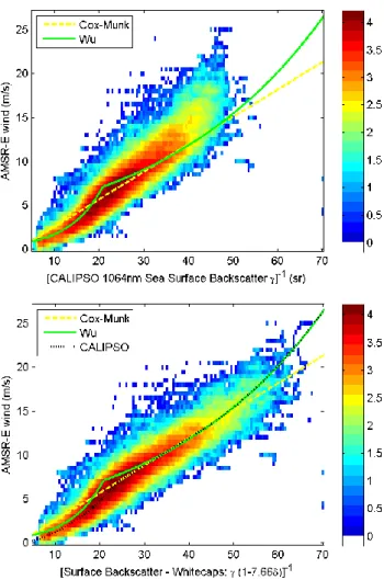
Fig. 2. Upper panel: 3-D histogram of CALIPSO sea surface lidar backscatter and collocated AMSR-E wind speed. Lower panel: 3-D histogram of CALIPSO sea surface lidar backscatter with white-cap correction and collocated AMSR-E wind speed. The colors are log10[number of occurrence]. Multiplying the total lidar
backscat-ter (co-polarization+cross-polarization) by the factor 1–7.66δ re-moves the cross-polarization component plus the whitecaps part of the co-polarization component (assuming the whitecaps has a 15% depolarization).
Figure 2 shows the relation between the AMSR-E wind speeds and the CALIPSO integrated lidar backscatter of ocean surface for the top 4% cleanest air for January of 2007. The cleanness is defined by 15-shot average lidar integrated atmospheric backscatter at both 532 nm and 1064 nm. The colors in the figure is log10[number of observations]. The
se-lection of the cleanest air regions is based on a 5 km running mean of the integrated atmospheric lidar backscatter. The ocean surface lidar backscatter is the sum of 532 nm surface parallel backscatter signal, with two-way atmospheric trans-mittance estimated from the lidar atmospheric backscatter profile. There is good correlation between the lidar backscat-ter and wind speed for wind speeds lower than 12 m/s. The ocean surface lidar backscatter and wind speed become less
correlated for stronger wind (upper panel of Fig. 2), when the lidar signal is contaminated by the backscatter from white-caps. Whitecaps can be considered as multiple scattering by spherical particles with sizes comparable to or greater than the light wavelength (Massel, 2007). Multiple scatter-ing of spherical particles can be characterized by the lidar depolarization ratio (Hu et al., 2006; Hu et al., 2007c). A correction for whitecaps and ocean sub-surface backscatter was done by assuming a 15% lidar depolarization of white-caps and coastal region 1064 nm sub-surface lidar backscat-ter. For wind speed larger than 12 m/s, the correlation be-tween AMSR-E wind speed and CALIPSO lidar backscat-ter increased from 0.36 to 0.69 afbackscat-ter this whitecap correction (lower panel). The 15the Full Stokes Monte Carlo model (Hu et al. 2001) with simplified optical properties of foam and whitecaps. A more sophisticated correction algorithm based on realistic foam and whitecaps simulation is in progress.
The wave slope variance σ2– wind speed U relations from Cox-Munk, Wu and the best fit from the CALIPSO/AMSR-E data are also plotted in the lower panel of Fig. 2 as the yellow, green and black curves, with the y-axis as wind speed and x-axis as the inverse of lidar backscatter, 1/γ , after whitecap correction. 1/γ is proportional to σ2(U ) as in Eq. (4).
The best fit is performed on the entire month’s worth of clear sky ocean surface lidar backscatter data, weighted by the uncertainties in 1064nm aerosol extinction optical depth. The best fit σ2−U relation from the CALIPSO/AMSR-E data, as illustrated in the lower panel of Fig. 2, is summa-rized in Eq. (5).
For wind speeds between 7 m/s and 13.3 m/s, Cox-Munk model agree well with the CALIPSO/AMSR-E data, as demonstrated in the lower panel of Fig. 2. For wind speed higher than 13.3 m/s, the Wu model is adopted in the new CALIPSO wind – wave slope relation, since it fits the data slightly better.
For wind speed less than 7 m/s, both the Cox-Munk model and the Wu model are biased. The Wu model over-estimates the wind speed by 1–2 m/s for wind speed between 3–9 m/s. And the Cox-Munk models over-estimate the wind speed by 1–2 m/s for wind speeds less than 5 m/s. For wind speeds less than 7 m/s, the square root of the wind speed is the unbiased fit of wave slope variance, σ2. As we discussed in the in-troduction, lidar sea surface backscatter is inversely propor-tional to the sqaure root of wave slope variance if the wave slope statistics is one dimensional Gaussian. If we assume a linear relation between slope variance and wind speed here, then the wave slope distribution is likely a one dimensional Gaussian distribution for wind speeds lower than 7 m/s. This implication can only be confirmed by collocated wind speed measurements together with multi-angle lidar measurements. With collocated ocean surface wind and sunglint satel-lite radiometer measurements, recent studies concur with Cox-Munk relation at moderate wind speeds while issues related to wind direction, low wind and high wind exist (Ebuchi and Kibu, 2002; Breon and Henriot, 2006; Li et al.,
2007). The nadir-pointing lidar is not sensitive to the wind direction related issues found in the sunglint measurements. Studying wind and slope variance relation using combined wind/lidar measurements can avoid uncertainty associated cloud/aerosol contaminaiton (Flamant et al., 1998).
3 Improving calibration with ocean surface lidar backscatter
Using ocean surface backscatter for space based lidar cal-ibration was first performed by Lidar In-space Technology Experiment (LITE) (Menzies, 1998) and Ice, Cloud and land Elevation Satellite (ICESat) (Lancaster et al., 2005). For CALIPSO, the ocean surface can be used for accurate cal-ibration, because we have access to:
– collocated AMSR-E wind speed; – accurate aerosol loading information; – improved wind speed - wave slope relation.
From Eq. (4),1γγ ≈−1σ2
σ2 , and from Eq. (5),
1σ2 σ2 ≈
1U U for wind speeds between 7 m/s and 13.3 m/s, so that the inverse of the lidar backscatter coefficient is seen to change linearly with wind speed. Within this wind speed regime, 10% certainty in lidar backscatter is thus equivalent to a 10% un-certainty in wave slope variance, as well as in wind speed.
For wind speeds less than 7 m/s 1γγ ≈−1U
2U, thus a 20%
uncertainty in wind speed is equivalent to about 10% uncer-tainty in the wave slope variance and in the lidar backscatter. Overall, 1 m/s wind speed uncertainty is equivalent to about 10% of uncertainty in both the wave slope variance and in the lidar backscatter.
The two largest sources of uncertainty in studying the wind speed – wave slope variance using sea surface lidar backscat-ter data are the estimation of two-way atmospheric transmit-tance and the uncertainty in the lidar calibration. Because the well-established molecular normalization technique can be employed, the calibration of CALIPSO’s 532 nm channel can be highly accurate. Signal-to-noise (SNR) considerations make this method unsuitable for use at 1064 nm. However, because the scattering efficiency of aerosols in the Earth’s at-mosphere is significantly less at 1064 nm than at 532 nm, the aerosol optical corrections required for the 1064 nm signals are much less uncertain than the corresponding corrections applied to the 532 nm channel.
The best combination of the 532 nm and 1064 nm surements to make the most accurate sea surface wind mea-surements is to retrieve wind speed using 1064 nm sea sur-face backscatter after calibration improvement. In this study, sea surface backscatter of CALIPSO lidar profiles with the smallest atmospheric backscatter is used as a target for im-proving lidar calibration,
– the 532 nm calibration is adjusted so that the latitudinal
dependence of sea surface lidar backscatter agrees with the theoretical lidar backscatter derived from AMSR-E wind speed.
– the 1064 nm calibration is adjusted so that the ocean
sur-face backscatter at both 532 nm and 1064 nm channels agrees.
Accurate CALIPSO lidar backscatter can help improve the understanding of the relation between wind speed and sea surface lidar backscatter. On the other hand, sea surface backscatter can be used as a target for the assessment of the lidar calibrations. As the molecular backscatter sig-nal at 1064 nm is very weak, the CALIPSO 1064 nm lidar backscatter cannot be calibrated to the same degree of ac-curacy as the backscatter at 532 nm. The acac-curacy of the CALIPSO 1064 nm calibration can be assessed by compar-ing the sea surface lidar backscatter at the two wavelengths. The sea surface lidar backscatter measurement at 1064 nm is 7.3% lower than the lidar backscatter at 532 nm because of the slight difference in refractive indices at 532 nm and 1064 nm (1.335 and 1.32, respectively). The relative differ-ence in atmospheric attenuation for the two channels can be well quantified for those cases when the lidar shots with col-located AMSR-E wind speeds are between 7 m/s and 9 m/s, and there are no clouds and very little aerosols above the sea surface (as determined by the range-resolved lidar returns).
The upper panel of Fig. 3 shows that the nighttime CALIPSO 1064 nm sea surface backscatter for January 2007 agrees well (to within 10%) with 532 nm sea surface backscatter at the middle and high latitudes of the south-ern hemisphere, and is a few percent weaker than 532 nm backscatter in the higher latitudes of the northern hemi-sphere. The attenuation caused by molecular scattering and absorptions at both wavelengths, as well as the detector tran-sient response differences between the two wavelengths, are all accounted for when computing the 532 nm/1064 nm li-dar sea surface backscatter ratios. The slight latitudinal de-pendence evidenced in the figure is likely a result of ther-mal changes that occur at the orbit terminator, and effect the alignment between the lidar’s transmitter and receiver in a slightly different manner for each of the two channels. This is part of the overall instrument calibration and future planned CALIPSO algorithm development should reduce this effect. Only night-time data are presented in this study. Applica-tion of a latitudinal correcApplica-tion for 1064 nm calibraApplica-tion (CG2R,
which is a linear fit of the 532 nm/1064 nm lidar sea surface backscatter ratios) can assure the consistency of 532 nm and 1064 nm lidar sea surface backscatter.
Sea surface lidar backscatter can also be used for the assessment of CALIPSO 532 nm lidar calibration. From Eq. (5), sea surface lidar backscatter can be computed from AMSR-E wind speed and should agree well with the li-dar CALIPSO 532 nm sea surface lili-dar backscatter measure-ments. The lower panel of Fig. 3 shows that, except for the
3598 Y. Hu et al.: Sea surface wind speed estimation from space-based lidar
Fig. 3. Upper Panel: Mean sea surface backscatter ratio of 532 nm and 1064 nm channels for the cleanest (4%, 2%, 1%) atmosphere. The 1064 nm channel recalibration is performed so that the sea sur-face lidar backscatter of the 532 nm and the 1064 nm channels agree with theory, while two-way atmospheric transmittance of the clean-est air can be accurately clean-estimated. Lower Panel: Mean sea surface 532 nm channel backscatter ratio of observation vs. theory. Here clean means that atmospheric (aerosol) backscatter is low.
tropics and the Arctic, the measured lidar backscatter val-ues are approximately 5% higher than the estimates obtained from the AMSR-E wind data. This small bias is probably due to the uncertainty of CALIPSO’s lidar calibration us-ing molecules as targets and the impact of the transient re-sponse of the CALIPSO photomultiplier tubes (PMT) (Hu et al., 2007a; Hu et al., 2007b; McGill et al., 2007). The sea surface 532 nm lidar backscatter measurements at the trop-ics are a few percent lower. This result is likely due to the lack of stratospheric aerosol treatment in CALIPSO calibra-tion process. The downward spike at 40N is likely due to the uncertainties in AMSR-E wind speed.
After applying the derived latitudinal dependence correc-tion (red curves in both the upper and lower panels of Fig. 3), the wave slope variance – wind speed relation can be further assessed by comparing CALIPSO 1064 nm sea surface lidar backscatter with AMSR-E wind. Atmospheric attenuation
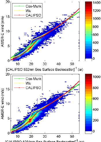
Fig. 4. 3-D histogram of single shot CALIPSO 532 nm (up-per panel) and 1064 nm (lower panel) sea surface backscatter vs. AMSR-E wind speed for lowest aerosol loadings (cleanest at-mosphere, with smallest 2% γatmos). The color represents the
frequency of occurrence, with the unit of [sr m/s]−1. The light blue, green and yellow curves are 1/γ as a function of wind speed
U, derived from Cox-Munk, Wu and CALIPSO-AMSR-E σ2–U -relations.
from aerosols is much weaker at 1064 nm wavelength than at 532 nm, reducing this source of error. The sea surface lidar backscatter at 1064 nm has less uncertainty associated with the estimation of two-way atmospheric transmittance.
Figure 4, which includes 2% of most cloud-and-aerosol-free ocean measurements for January 2007, shows that the wave slope variance – wind speed relation described in Eq. (5) is indeed a good fit of the corrected 1064 nm (lower panel) CALIPSO sea surface lidar backscatter and AMSR-E wind speed data. However, there is larger uncertainty of aerosol two-way transmittance at 532 nm. In general, the relation between 532 nm lidar backscatter and AMSR-E wind speed (lower panel of Fig. 4) still agrees with AMSR-Eq. (5). There are more 532 nm lidar data points below the curves of Eq. (5), indicating a possible bias. These data points are
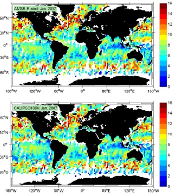
Fig. 5. Monthly mean (January 2007) wind speeds derived from CALIPSO 1064 nm (lower panel), and collocated monthly mean AMSR-E wind speed (upper panel). The colors are wind speed (M/s).
found to be occurring mostly in areas where there are ab-sorbing aerosols, where aerosol extinction optical depth is slightly under-estimated from atmospheric lidar backscatter signal.
4 Applying the U − σ2-relation to derive wind speed from CALIPSO 1064 nm data
The wind speed – wave slope variance relation derived from the CALIPSO clear sky sea surface lidar backscatter and AMSR-E wind speed data, as described in Eq. (5), can be applied for measuring ocean surface wind speed using space-based lidar measurements, wherever/whenever the attenua-tion of the atmosphere can be assessed with sufficient confi-dence.
For clear sky with relatively low aerosol loading, the at-mospheric attenuation for 1064 nm CALIPSO lidar measure-ments can be estimated from the range-resolved profile of at-tenuated backscatter coefficients, and thus wind speed can be well estimated. The impact of whitecaps on 1064 nm sea sur-face backscatter is effectively removed by assuming a 15% depolarization introduced by the white caps, and the white-cap depolarization ratios at 532 nm and 1064 nm are identi-cal.
Fig. 6. Lower panel: histogram of wind speed difference between CALIPSO and AMSR-E for single CALIPSO lidar shot (blue) and 10 km CALIPSO average. The colors are the number of occurrence
F. The unit of the y-axis is counts per bin. Upper panel: Map of wind speed difference between CALIPSO and AMSR-E. The unit of the color scale is m/s
The lower panel of Fig. 5 shows the monthly maps of the CALIPSO wind speed measurements from 1064 nm lidar ocean surface backscatter, while the upper panel shows the collocated wind speeds reported by AMSR-E. The monthly mean CALIPSO wind speed agrees well with the AMSR-E wind speed, except in those regions affected by dense dust and smokes (e.g., off of Africa), where the atmospheric at-tenuation may have been under-estimated in the lidar data processing. The upper panel of Fig. 6 is the difference be-tween the two maps.
The lower panel of Fig. 6 shows that the rms difference between AMSR-E wind speed and wind speed derived from the single CALIPSO lidar shot is 1.2 m/s. The rms difference reduces to 0.86 m/s when we average the CALIPSO lidar data along track to 10 km (30 lidar profile). Considered on a global scale, there is no systematic bias between CALIPSO and AMSR-E wind speeds. However, as shown in the up-per panel of Fig. 6, the CALIPSO wind speed estimates at higher latitudes are ∼0.5 m/s lower than those reported by AMSR-E, which is probably a combination of uncertainties
3600 Y. Hu et al.: Sea surface wind speed estimation from space-based lidar
in CALIPSO calibration and whitecap correction, as well as potential AMSR-E wind speed bias associated with sea ice and drizzle contamination.
The blank regions in Fig. 6 are the regions with too much clouds and aerosols so that we did not perform the lidar re-trievals.
5 Summary and discussion
Using the collocated CALIPSO sea surface lidar backscatter measurements and the wind speeds reported in the AMSR-E data products, we have studied the relationship between wave slope variance and surface wind speed on a global scale. For wind speeds between 7 m/s and 13.3 m/s, the σ2–U -relation derived from the CALIPSO sea surface lidar backscatter and AMSR-E wind data agrees well with the linear relation es-tablished by Cox and Munk. For wind speeds higher than 13.3 m/s, the σ2–U -relation derived from the CALIPSO li-dar backscatter and AMSR-E wind data agrees with the log-linear relation derived by Wu. For wind speeds lower than 7 m/s, the assumption of an isotropic, two dimensional Gaus-sian wave slope distribution results in a linear relationship between wave slope variance and square root of wind speed. If the wave slopes obey a one-dimensional Gaussian distribu-tion for wind speed below 7 m/s, the slope variance is again seen to be a simple linear relation.
Applying this σ2−U relation, global sea surface wind speed can be derived from both the CALIPSO 1064 nm and 532 nm sea surface backscatter, which are defined as the inte-grated lidar surface signal divided by two-way atmospheric transmittance. The two-way atmospheric transmittance can be estimated directly from the CALIPSO atmospheric lidar backscatter profile. The effects of whitecaps and the con-tributions from subsurface ocean signals are effectively re-moved by using the CALIPSO 532 nm depolarization mea-surements. The global monthly mean wind speed distribu-tion derived from CALIPSO agrees well with the AMSR-E wind product. The rms difference is 1.2 m/s between the single lidar shot CALIPSO wind speed with the AMSR-E wind (20 km resolution). The rms difference drops to 0.86 m/s when the wind speed is derived from CALIPSO li-dar backscatter averaged to 10 km along track.
This study demonstrates that sea surface wind speed can be accurately measured from space-based lidar measure-ments. The outcome of this study can help the calibration of space-based lidars, since the sea surface lidar backscatter sig-nal is relatively strong and thus reduces requirements on sen-sitivity and dynamic range for the lidar. Apart from lidar cal-ibration concerns, atmospheric attenuation by aerosols is the largest source of uncertainty in retrieving wind speed. The wind speed retrieval uncertainty associated with the atmo-spheric attenuation would be reduced significantly by using lidar measurements operating at mid-infrared wavelengths where the aerosol contribution to the backscatter is
signif-icantly less. The wind speed retrieval can also improve when aerosol optical depth derived from other sensors such as MODIS are considered.
The microwave-based measurement of sea surface winds can be carried out over a wider range of weather conditions than the lidar due to the greater ability to penetrate through clouds. Space based lidar can make accurate measurements over a small (for example, 70 m for single shot) footprint, which would allow measurements closer to coastlines, and potentially in lakes, from space. The smaller footprint would allow the divergence and curl related to ocean stress to be estimated over smaller areas (Chelton et al., 2000). Cross-validation between ocean surface wind speeds derived from space based microwave radiometer and lidar measurements can help assess uncertainties of microwave radiometer de-rived wind speeds associated with issues such as calibration, raindrops, drizzles and sunglint. A space-based lidar has an advantage over standard visible imagery for measuring ocean winds because it can also measure the atmospheric attenua-tion and estimate sea state, reducing errors. The lidar can also make both day and night measurements. Daytime wind speed can be slightly less accurate due to larger uncertainties in calibrations and aerosol corrections as a result of smaller SNR of aerosol backscatter. The day/night SNR difference of ocean surface backscatter is small because the SNRs for both clear day/night are in the hundreds and CALIPSO nadir track is away from sunglint.
As the sea surface lidar backscatter is highly sensitive to atmospheric attenuation, this study indicates that the sea surface backscatter could potentially be used to derive ac-curate values of atmospheric column extinction (absorp-tion+scattering) optical depth using collocated CALIPSO backscatter and AMSR-E wind speed. This topic will be ex-plored further in a subsequent, companion paper.
Acknowledgements. This study is sponsored by NASA CALIPSO/CloudSat A-train and MIDAS project of NASA Radiation Science Program and Ocean Biogeochemistry Program under H. Maring, P. Bontempi and D. Anderson.
Edited by: Q. Fu
References
Barrick, D. E.: Rough surface scattering based on the specular point theory, IEEE Trans. Antennas Propag., AP-16, 449–454, 1968. Breon, F. M., and Henriot, N., Spaceborne observations of ocean
glint reflectance and modeling of wave slope distributions, J. Geophys. Res., 111, C06005, doi:10.1029/2005JC003343, 2006. Bufton, J., Hoge, F., and Swift, R.: Airborne measurements of laser backscatter from the ocean surface, Appl. Optics, 22, 2603– 2618, 1983.
Chelton, D. B., Freilich, M. H., and Esbensen, S. K: Satellite obser-vations of the wind jets off the Pacific coast of Central America,
Part I: Case studies and statistical characteristics, Mon. Weather Rev., 128, 1993–2018, 2000.
Cox, C. and Munk, W.: Measurement of the Roughness of the Sea Surface from Photographs of the Sun’s Glitter, J. Opt. Soc. Am., 14, 838–850, 1954.
Ebuchi, N., and Kizu, S.: Probability distribution of surface wave slope derived using sun glitter images from Geostationary Me-teorological Satellite and surface vector winds from scatterome-ters, J. Oceanogr., 58, 477–486, 2002.
Ebuchi, N.: Evaluation of marine surface winds observed by Sea-Winds and AMSR on ADEOS-II, J. Oceanography, 62, 293–301, 2006.
Flamant, C., Trouillet, V., Chazette, P., Pelon, J.: Wind speed de-pendence of atmospheric boundary-layer optical properties and ocean surface reflectance as observed by backscatter lidar, J. Geophys. Res.-Oceans, 103, 25137–25158, 1998.
Freilich, M. and Vanhoff, B., The Relationship between Winds, Sur-face Roughness, and Radar Backscatter at Low Incidence An-gles from TRMM Precipitation Radar Measurements, J. Atmos. Ocean. Tech., 20, 549–562, 2003.
Ginneken, B., Stavridi, M., and Koenderink, J.: Diffuse and Specu-lar Reflectance from Rough Surface, Appl. Optics, 37, 130–139 , 1998.
Hu, Y., Winker, D., Yang, P., Baum, B., Poole L., and Vann, L.: Identification of cloud phase from PICASSO-CENA lidar depo-larization: A multiple scattering sensitivity study, J. Quant. Spec-tros. Radiat. Trans., 70, 569–579, 2001.
Hu, Y., Liu, Z., Winker, D., Vaughan, M., Noel, V., Bissonnette, L., Roy, G., and McGill, M.: A simple relation between lidar multi-ple scattering and depolarization for water clouds, Opt. Lett., 31, 1809–1811, 2006.
Hu, Y., Vaughan, M., Liu, Z., Lin, B., Yang, P., Flittner, D., Hunt, B., Kuehn, R., Huang, J., Wu, D., Rodier, S., Powell, K., Trepte, C., and Winker, D.: The depolarization – attenuated backscatter relation: CALIPSO lidar measurements vs. theory. Opt. Express, 15, 5327–5332, 2007a.
Hu, Y.,Powell, K., Vaughan, M., Trepte, C., Weimer, C., Beheren-feld, M., Young, S., Winker, D., Hostetler, C., Hunt, W., Kuehn, R., Flittner, D., Cisewski, M., Gibson, G., Lin, B., and Mac-Donald, D.: Elevation-In-Tail (EIT) technique for laser altimetry, Opt. Express, 15, 14 504–14 515, 2007b.
Hu, Y.: Depolarization Ratio – Effective Lidar Ratio Relation: Theoretical Basis for Space Lidar Cloud Phase Discrimination, Geophys. Res. Lett., 34, L11812, doi:10.1029/2007GL029584, 2007c.
Lancaster, R. S., Spinhirne, J. D., and Palm, S. P.: Laser pulse reflectance of the ocean surface from the GLAS satellite lidar, GEO. RES. LETT., 32, L22S10, doi:10.1029/2005GL023732, 2005.
Li, L., Fukushima, H., Suzuki, K., and Suzuki, N.: Optimization of Cox and Munk sun-glint model using ADEOS/II GLI data and SeaWinds data, SPIE – The International Society for Optical Engineering, 6680, P668006, doi:10.1117/12.732779, 2007. Liu, Y., Su, M., Yan, X., Liu, W. T.: the Mean Square Slope of
Ocean Surface Waves and Its Effects on Radar Backscatter, J. Atmos. Ocean. Tech., 17, 1092–1105, 2000.
Massel, S.: Ocean Waves Breaking and Marine Aerosol Fluxes, Springer, 38, 328 p., doi:10.1007/978-0-387-69092-6, 2007. McGill, M. J., Vaughan, M. A., Trepte, C. R., Hart, W. D., Hlavka,
D. L., Winker, D. M., and Kuehn, R.: Airborne Validation of Spatial Properties Measured by the CALIPSO Lidar, J. Geophys. Res., 112, D20201, doi:10.1029/2007JD008768, 2007.
Menzies, R., Tratt, D., and Hunt, W.: Lidar In-space Technol-ogy Experiment Measurements of Sea Surface Directional Re-flectance and the Link to Surface Wind Speed, Appl. Optics, 37, 5550–5559, 1998.
Platt, C.: Lidar and radiometric observations of cirrus clouds, J. Atmos. Sci., 30, 1191–1203, 1973.
Shaw J. and Churnside, J.: Scanning-laser glint measurements of sea-surface slope statistics, Appl. Optics, 36, 4202–4213, 1997. Tratt, D., et al.: Airborne Doppler Lidar Investigation of the
Wind-Modulated Sea-Surface Angular Retroreflectance Signa-ture, Appl. Optics, 33, 6941–6950, 2002.
Wentz, F. and Meissner, T.,: AMSR Ocean Algorithm Theoreti-cal Basis Document, Version 2. Remote Sensing Systems, Santa Rosa, CA, 2000.
Wentz, F., Gentemann, C., and Ashcroft, P.: On-orbit calibration of AMSR-E and the retrieval of ocean products, 83rd AMS Annual Meeting, American Meteorological Society, Long Beach, CA, 2003.
Wu, J.: Mean square slopes of the wind-disturbed water surface, their magnitude, directionality, and composition, Radio Sci., 25, 37–48, 1990.