HAL Id: hal-00328432
https://hal.archives-ouvertes.fr/hal-00328432
Submitted on 18 May 2006
HAL is a multi-disciplinary open access
archive for the deposit and dissemination of
sci-entific research documents, whether they are
pub-lished or not. The documents may come from
teaching and research institutions in France or
abroad, or from public or private research centers.
L’archive ouverte pluridisciplinaire HAL, est
destinée au dépôt et à la diffusion de documents
scientifiques de niveau recherche, publiés ou non,
émanant des établissements d’enseignement et de
recherche français ou étrangers, des laboratoires
publics ou privés.
UTLS air composition – Part 2: Ozone budget in the
TTL
E. D. Rivière, V. Marécal, N. Larsen, S. Cautenet
To cite this version:
E. D. Rivière, V. Marécal, N. Larsen, S. Cautenet. Modelling study of the impact of deep convection on
the UTLS air composition – Part 2: Ozone budget in the TTL. Atmospheric Chemistry and Physics,
European Geosciences Union, 2006, 6 (6), pp.1598. �10.5194/acp-6-1585-2006�. �hal-00328432�
www.atmos-chem-phys.net/6/1585/2006/ © Author(s) 2006. This work is licensed under a Creative Commons License.
Chemistry
and Physics
Modelling study of the impact of deep convection on the UTLS air
composition – Part 2: Ozone budget in the TTL
E. D. Rivi`ere1,*, V. Mar´ecal1, N. Larsen2, and S. Cautenet3
1Laboratoire de Physique et Chimie de l’Environnement/CNRS and Universit´e d’Orl´eans, 3A avenue de la Recherche
Scientifique, 45071 Orl´eans cedex 2, France
2Danish Meteorological Institute, Division of Middle Atmosphere Research, Lyngbyvej 100, DK-2100, Copenhagen,
Denmark
3Laboratoire de M´et´eorologie Physique/CNRS-OPGC/Universit´e Blaise Pascal, 24 Avenue des Landais, 63177 Aubi`ere
cedex, France
*now at: Groupe de Spectrom´etrie Mol´eculaire et Atmosph´erique UMR 6089 and Universit´e de Reims Champagne-Ardenne,
Facult´e des Sciences, Bˆat. 6, case 36, BP 1039, 51687 Reims Cedex 2, France
Received: 29 March 2005 – Published in Atmos. Chem. Phys. Discuss.: 23 September 2005 Revised: 6 February 2006 – Accepted: 15 March 2006 – Published: 18 May 2006
Abstract. In this second part of a series of two papers which
aim to study the local impact of deep convection on the chemical composition of the Upper Troposphere and Lower Stratosphere (UTLS), we focus on ozone simulation results using a mesoscale model that includes on-line chemistry. A severe convective system observed on 8 February 2001 at Bauru, Brazil, is studied. This unorganised convective sys-tem is composed of several convective cells that interact with each other. We show that there is an increase in the ozone concentration in the tropical transitional layer (TTL) in the model during this event, which is compatible with ozone sonde observations from Bauru during the 2004 convective season. The model horizontal variability of ozone in this layer is comparable with the variability of the ozone sonde observations in the same area. The calculation of the ozone budget in the TTL during a 24 h period in the area of the con-vective system shows that the ozone behaviour in this layer is mainly driven by dynamics. The horizontal flux at a specific time is the main contribution in the budget, since it drives the sign and the magnitude of the total ozone flux. However, when averaged over the 24 h period, the horizontal flux is smaller than the vertical fluxes, and leads to a net decrease of ozone molecule number of 23%. The upward motions at the bottom of the TTL, related to the convection activity is the main contributor to the budget over the 24 h period since it can explain 70% of the total ozone increase in the TTL, while the chemical ozone production inside the TTL is estimated to be 29% of the ozone increase, if NOxproduction by lightning
Correspondence to: E. D. Rivi`ere ([email protected])
(LNOx)is taken into account. It is shown that downward
motion at the tropopause induced by gravity waves gener-ated by deep convection is non negligible in the TTL ozone budget, since it represents 24% of the ozone increase. The flux analysis shows the importance of the vertical contribu-tions during the life time of the convective event (about 8 h). The TTL ozone is driven out of the domain horizontally by the convective outflow during this period, limiting the ozone increase in this layer.
1 Introduction
It is now well accepted that deep convection plays an im-portant role in the redistribution of chemical species from the boundary layer up to the upper troposphere (e.g. Dick-erson et al., 1987; Thornton et al., 1997; Wang and Prinn, 2000). Some of the species transported to a few kilome-tres below the tropopause might be important for the ozone chemistry budget, both for its production in the troposphere (NOx, OVOC, CO, HOx), and for its destruction in the
strato-sphere (e.g. Cly, Bry, NOx). The main way for species
to reach the stratosphere is to cross the tropical tropopause (Holton et al., 1995), or possibly to cross laterally the extra-tropical tropopause (e.g. Ray et al., 1999; Schoeberl, 2004). Knowing the chemistry and composition of the layer below the tropical tropopause, called the tropical transitional layer (TTL), is a necessary step in determining the amount of each chemical compound entering the stratosphere. Once in the tropical stratosphere, all chemical compounds will be trans-ported by the general Brewer-Dobson circulation to higher
latitudes (Brewer, 1949), potentially affecting the global ozone budget.
Many chemical species (O3, NOx, HOx, other ozone
pre-cursors, halogen species including very short life substances) need to be studied throughout the whole troposphere to bet-ter understand the TTL chemical composition. Among these species ozone is of specific interest for several reasons.
Firstly, its behaviour in the TTL is not fully understood. From several balloon-borne ozone observations, it has been shown that the TTL is characterised by an increase of ozone with altitude (measurements published in Taupin et al., 1999; Pundt et al., 2002; V¨omel et al., 2002; Thompson et al., 2003) that extends in the stratosphere. On one hand, us-ing climatological profiles, Folkins et al. (2002) highlighted a typical “S-shaped” vertical profile of ozone in the tropi-cal troposphere (consisting of an increase in the lower tro-posphere, a slight decrease in the middle troposphere and an increase in the upper troposphere), and explained this tendency with a simple 1-D model. This model only takes into account the contributions of advection, convection, and chemical ozone production. Since the tropospheric processes taken into account in the model of Folkins et al. (2002) are enough to describe the climatological shape of the tropo-spheric ozone profile, it can be concluded that the increase of ozone in the TTL is not due to stratospheric production of ozone. On the other hand, on an individual measurement approach during the wet season (V¨omel et al, 2002; Pundt et al., 2002; Dessler et al., 2002), the behaviour of O3in the
TTL can be less regular and can lead to a local maximum or a sharp increase in the vertical profile. This behaviour has not been fully explained yet, even though V¨omel et al. (2002) explained one of these events with a passing Kelvin wave.
Secondly, considering the lifetime of ozone in the upper troposphere and the lower stratosphere (UTLS) due to chem-ical loss alone (typchem-ically longer than a month), the O3
con-centration is then determined by transport and chemical pro-duction (WMO, 2003). While not a perfect tracer, this prop-erty makes ozone a relatively good indicator of vertical trans-port from the surface up to the TTL. On this basis Dessler et al. (2002) combined O3with CO measurements, and Folkins
et al. (2002) used an O3profile to infer the level of convective
outflow.
Finally, ozone is one of the most measured species in the tropical upper troposphere. This is helpful for conducting chemistry studies in the upper troposphere, even if the ozone chemistry is relatively complex.
In this context, the aim of this series of two papers is to study the chemical composition of the UTLS associated with a severe deep convective event over Brazil. For this purpose, we are using 3-D simulations performed with a mesoscale model coupled on-line with a chemistry model. The case studied here is the convective event observed on 8 February 2001 in the region of Bauru, State of S˜ao Paulo, in the frame of the preparation campaign of the EC funded HIBISCUS project. The aim of HIBISCUS is to study the impact of
the tropical region on ozone on a global scale. The reasons for choosing this case study are the following. Firstly, the severity of the convection, almost reaching the tropopause, makes this case particularly interesting for studying the im-pact of deep convection on the TTL chemical composition. Secondly, this convective case is composed of a cluster con-vective cells that possibly interact with each others. Sev-eral modelling studies aiming at quantifying the impact of deep convection on the upper troposphere composition have already been published (Yin et al., 2001; Wang and Prinn, 2000; Barth et al., 2001; Tulet et al., 2002, DeCaria et al., 2005). Most of them studied either an individual convec-tive cell or a well organised system (tropical or not). The present paper focuses on a more complex type of system: a non-organised and extreme tropical convective system. The first paper of the series (Mar´ecal et al., 2006) is devoted to the description of the event, the validation of the meteoro-logical simulation results, and the study of the ozone pre-cursor distribution in the UTLS associated with this severe event. This paper reports the following results. The CO re-sults are compatible with the airborne measurements previ-ously performed over Brazil in another year during the con-vective season in the upper troposphere, and are also com-patible with the MOPITT satellite monthly average data for February 2001. The NOx simulation, taking into account
a parameterisation of NOx production by lightning, shows
that this process strongly affects the NOxdistribution in the
layer at 6–16 km, with a maximum mean value of 2 ppbv at 12.5 km in the area of convection. Local maxima in the Non-Methane volatile organic compounds (VOCs) were also com-puted by the model and were in the altitude range 8 to 12 km for propene and isoprene, and in the altitude range 7–15 km for ethane. These relatively large values of Non-Methane VOCs in the upper troposphere, combined with high contents of HOx and HOx precursors, mainly due to vertical
trans-port by deep convection, might affect the ozone budget in the TTL.
The aim of this second paper is to study the impact of deep convection on the ozone behaviour in the UTLS with partic-ular attention paid to its budget in the TTL. This analysis is based on the same short time simulation of the convective system as in Mar´ecal et al. (2006). In particular, we would like to answer the following questions:
Is the model able to reproduce typical TTL ozone be-haviour? What is the relative contribution of the dynamics and of the chemical processes to the upper tropospheric O3
distribution? What is the relative contribution of horizontal and vertical dynamics? Does the NOxproduction by
light-ning directly affect the ozone concentration in the TTL? In Sect. 2, we present the simulation results for ozone. Section 3 discusses the validation of the ozone results us-ing measured profiles published in the literature and DMI O3
sonde measurements performed from Bauru during the HI-BISCUS field campaign in 2004. Section 4 is devoted to the estimation of the impact of the chemical ozone production on
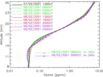
Fig. 1. Temporal evolution of the O3 mean profile in the
verti-cal range (8 km; 26 km) computed at regular 4 h time intervals by RAMS in Grid 2 between 8 February 2001 at 00:00 UT and 9 Febru-ary 2001 at 04:00 UT. The initial state is also shown (black line). The horizontal scale is logarithmic.
ozone in the TTL, while Section 5 discusses the dynamical and chemical budget of ozone in this layer. The main con-clusions and perspectives of this paper are given in Sect. 6.
2 Ozone simulation results
2.1 Simulation summary
Since the model and the simulation setup are fully described in Mar´ecal et al. (2006), we just briefly summarise the char-acteristics of the simulation in the present paper. The model used is the RAMS mesoscale model (Pielke et al., 1992; Cot-ton et al., 2003) coupled on-line with a condensed chemistry module originally developed by Aumont et al. (1996). The coupled model will be referred to hereafter as the RAMS-chemistry model (e.g. Taghavi et al., 2004). A compara-ble mesoscale model with online chemistry was successfully used by Tulet et al. (2002) to simulate the redistribution of ozone by a convective system observed at mid-latitudes. The chemical package of the RAMS-chemistry model takes ac-count of 29 species with 72 gas phase reactions. Aqueous phase chemistry for 9 species is included. Firstly this allows the passage of these species from the gas phase to the liquid phase, and vice versa. Secondly, liquid phase reactions from Gr´egoire et al. (1994) are included. The model accounts for the NOxproduction by lightning (LNOx)using the
param-eterisation of Pickering et al. (1998) and references therein. The initialisation of the chemical species is deduced from the chemistry transport model MOCAGE (Peuch et al., 1999). A 42-h simulation has been used, starting from 7 February 2001, 12:00 UT. The run is performed using two nested grids. The fine grid (referred later as Grid 2) has a horizontal grid
Fig. 2. Same as in Fig. 1 but for O3standard deviation normalised
by the mean vertical profiles in Fig. 1.
spacing of 4 km×4 km and a vertical resolution of 0.5 km in the UTLS, covering 628 km×608 km, including the Bauru and S˜ao Paulo areas. The maximum convective activity in the model is reached at 22:00 UT on 8 February. Two sim-ulations with different chemistry were performed. The first one, referred to as the “reference simulation”, includes NOx
production by lightning, except during the 12 first hours of the simulation. The spin-up period, that is, the initial pe-riod needed by the model to reach equilibrium, is evaluated to be 12 h. In order to avoid NOx production by lightning
associated with unrealistic convective ascent during the spin-up period, the LNOxparameterisation has been switched-off
during this period for the “reference” run. The other run, referred to hereafter as the “no LNOx” simulation, does not
take into account NOxproduction by lightning.
2.2 Vertical structure
The evolution of the mean ozone profile in Grid 2 between 8 February 00:00 UT and 9 February 04:00 UT at 4 h incre-ments, corresponding to the “reference” simulation, is shown in Fig. 1. The results of the “no LNOxsimulation” are also
plotted for two specific times. The corresponding standard deviations normalised by the average values are plotted in Fig. 2. For each profile, we can broadly distinguish 3 differ-ent layers. The first layer, in the altitude range 8 to 13 km is characterised by an almost constant value with altitude (∼40 ppbv) and a relatively weak change with time. As an indication, 40 ppbv is the typical mean value of ozone at the ground level during the simulations. The corresponding vari-ability is relatively low (typically about 12%), with values increasing with altitude. The second layer, from 13 km alti-tude up to the tropopause (∼17 km in our case) corresponds to the beginning of the O3 mixing ratio increase with
alti-tude, even for the initial time profile. This behaviour is typ-ical of the TTL and the range of this second layer matches
well the altitude range given by the several definitions of the TTL. Furthermore, the analysis of the lapse rate simulated by the model shows a change in the lapse rate vertical structure from 13 km. Above this height, there is a constant increase up to 22 km. This change of the lapse rate vertical structure at 13 km is compatible with the definition of the bottom of the TTL according to Sherwood and Dessler (2000). Thus in the following, we will call the layer between 13 km and the tropopause the TTL. In the simulations, the TTL exhibits an important evolution of O3with time. In this layer, relatively
high values of the standard deviation are found. However, different shapes of the variability profile are found depend-ing on time. The third layer, above 17 km, corresponds to the stratosphere and is characterised by an ozone increase with altitude and a very weak time evolution. The variability in the stratosphere is much lower than in the TTL, with values typically below 10% and a tendency to decrease with alti-tude.
2.3 Time evolution
In the first layer (8 to 13 km), the changes of ozone concen-tration with time are weak. In the afternoon of 8 February 2001, an increase of ozone is found in the model. Concur-rently, a decrease of ozone is found after sunset. These fea-tures might be related to the O3production cycle in the
pres-ence of ozone precursors. Mar´ecal et al. (2006) have shown that convective activity brings large amounts of ozone pre-cursors to the upper troposphere. Therefore, ozone is chem-ically produced during daytime while sunset corresponds to the time when ozone is chemically destroyed. The dynam-ics might also play a role in this time evolution. Particularly, the ozone variability increases with time and is likely due to the enhancement of the convection activity with time. Both dynamical and chemical effects will be further analysed in Sects. 4 and 5.
The TTL exhibits the most significant variation with time during the convective event. It is worth noting that a compar-ison of the initial state (solid black line) and the profile 12 h later (solid green line) shows that there is no significant dif-ference in the mean profile over this period (Fig. 1). This is correlated with a weak convective activity in both the model and the observations from the Bauru radar. The variability for 7 February 12:00 UT and for 8 February 00:00 UT is also similar, differing by only 4 percentage points at the most. These differences are probably due to dynamical processes. The mean profile for 8 February at 04:00 UT is not signifi-cantly different from the initial state, even though there is a slight increase in ozone in the layer range 15–17 km.
From this time, above 14.5 km, there is a continuous in-crease with time in the mean ozone mixing ratio in the TTL, reaching a maximum on 9 February at 04:00 UT. The increase between 8 February 20:00 UT and 9 February 04:00 UT is greater than for other time intervals, while there is only a slight increase between 16:00 and 20:00 UT on 8
February 2001. There is a time decrease in the mean ozone mixing ratio only in the lower part of the TTL (from 13 km to 14.5) over the period 8 February 20:00 UT to 9 Febru-ary 04:00 UT. The time increase in the ozone amount in the TTL leads to a specific shape in the vertical ozone profile for 9 February at 04:00 UT. This disturbed behaviour in the TTL is characterised by a local inflection in the increase of ozone, which is different from the initial profile for which the derivative of ozone with respect to altitude was mono-tonic. In the TTL, the variability tendency starts with a de-crease with time (until 8 February at 04:00 UT) followed by an increase until 8 February 16:00 UT. Between 16:00 UT and 20:00 UT, the variability is roughly constant with altitude in the TTL, oscillating vertically around a 17% value. For 9 February at 00:00 UT and 04:00 UT, the TTL variability ex-hibits a specific behaviour with two local maxima at 14 km (21%) and 16.8 km (18%) and a local minimum in the mid-dle of it (about 10% at 14.8 km). This could indicate that the evolution of the ozone in the TTL is driven by two different processes at the top and at the bottom of the TTL.
In the lower stratosphere, the mean profile remains un-changed with time up to 20 km. The corresponding variabil-ity, which decreases with altitude, does not evolve signifi-cantly with time. Above this level, there is a slight increase on mean ozone and corresponding variability with time from 16:00 UT on 8 February.
Two mean profiles (variability, respectively) correspond-ing to the “no LNOx simulation” are also plotted in Fig. 1
(Fig. 2, respectively). 8 February at 08:00 UT is the lat-est time for which no differences appear between the pro-files from the “reference” and “no LNOx” simulations. On
9 February at 00:00 UT, the differences in the mean and variability profiles between the simulations with and with-out LNOxare large. These differences occurred in the range
9.5–14 km. This layer corresponds to the layer of the max-imum of NOxproduced by lightning (see Fig. 7 in Mar´ecal
et al., 2006). On average, the enhancement of ozone due to LNOx reaches 8% in this layer. This result is consistent
with the tendency given previously by the modelling stud-ies of Jourdain (2003) and Labrador et al. (2004) that were based on a different approach. Using a global scale chem-istry transport model which was run for a one year period, Labrador et al. (2004) estimated the tropospheric burden of O3enhancement due to LNOx to be 14%. Jourdain (2003)
using a global circulation model which was run to give a sim-ulation for one month, estimated the contribution of LNOxto
the O3enhancement over Brazil for the month of January to
be 10 to 15%.
For any other altitude than [9.5 km, 14 km], including the disturbed layer of the TTL, the simulations with and with-out LNOxsuperimpose in Fig. 1. This means that the large
increase of ozone in the TTL is not due entirely to the chem-istry associated with enhanced NOx from lightning.
How-ever, this does not rule out the potential role of the chemistry in producing the increase of O3 for this layer since it has
been shown in Mar´ecal et al. (2006) that ozone precursors were present in this range of altitude, even in the “no LNOx”
simulation.
In order to evaluate the validity of the simulation, we com-pare the results with measurements performed in Brazil dur-ing the convective season in the next section.
3 Evaluation of the model results
Since no ozone sonde or balloon-borne measurements were available in the Bauru area during the simulation period, we have used for comparison, profiles from ozone sondes launched from Bauru during February 2004. In our analysis, ozone sondes were preferred to balloon-borne remote sens-ing measurements because the latter type of instrument uses lines of sight of several hundred kilometres for profile re-trieval, which induces a horizontal resolution that is coarser than the scale of a convective system. Since our aim is to study the impact of convection on the chemical distribution on a local scale, in situ measurements were used.
3.1 DMI Ozone measurements
In the context of the HIBISCUS 2004 campaign, ozone son-des were launched regularly from Bauru between 10 Febru-ary and 24 FebruFebru-ary 2004. Standard electrochemical concen-tration cells (ECC) ozone sondes were applied, using 3 ml. 1% KI-cathode solutions, with an estimated ozone measure-ment accuracy of about 5% (Komhyr et al., 1995).
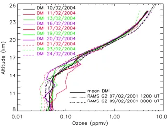
A total of 10 profiles were obtained from the ground up to 26–27 km. They depict a wide range of different mete-orological situations with respect to convection (close to or far from the convection, after or before a convective event). Thus, this set of measurements should help in evaluating our simulation, since inside the RAMS Grid 2 for a specific time, a wide range of situations with respect to the convection ac-tivity is also encountered. The 10 ozone profiles are shown in Fig. 3 for the vertical range 8 km to 26 km. To provide a comparison with the RAMS-chemistry results, the simulated profiles for the “reference” run for 7 February at 12:00 UT (initial time) and for 9 February at 00:00 UT are also shown. The mean profile from all the measurements was calculated and is given in Fig. 3. To provide a better comparison, the measurements were averaged over the RAMS vertical grid.
The 10 profiles are different, but generally the following characteristics are common. Firstly, the ozone profiles are generally almost constant with altitude up to around 13 km. Then the ozone mixing ratio starts to increase with height, well below the tropopause, as already observed in previously published measurements in the tropics (Pundt et al., 2002; Thompson et al., 2003; Vomel et al., 2002; Folkins et al., 2002). This corresponds to the TTL. For some DMI O3
sonde profiles, this layer can be highly disturbed, as shown by a local ozone maximum in the TTL (11, 16 and 17
Febru-Fig. 3. DMI sonde O3measurements from Bauru, Brazil, during
HIBISCUS 2004, expressed in the same vertical resolution as the RAMS model. The date of each launch is given in the figure. Also shown are the mean profile of all the measurements (black thick solid line), the mean vertical profiles of ozone computed by RAMS in Grid 2 at 12:00 UT on 7 February 2001 (initial state), and at 00:00 UT on 9 February 2001 for the “reference” run. The hori-zontal scale is logarithmic.
ary). Finally almost all the profiles superimpose in the lower stratosphere (∼ above 17 km) where the ozone increases with altitude. Only 2 profiles (23 February 2004 and 24 February 2004) differ significantly from the others above 20 km. The first, (DMI 23/02/2004) shows the lowest amount of all the measurements, while the second (DMI 24/02/2004) shows a much higher value of O3than all others. This is possibly due
to the location of the sonde when it was in the stratosphere: a more southern location would sample a higher content of ozone for the same altitude, while a position closer to the equator would lead to a lower amount. Since the sondes did not carry GPS receivers, it was not possible to check their latitudinal positions.
3.2 Model-measurements comparison
The initial state described by the model is in the range of the DMI measurements for any altitude, showing that the initial-isation used is realistic (Fig. 3). The initial profile is typical of the upper part of the “S-shaped” climatological profile re-ported in Folkins et al. (2002). The simulation results for 9 February 00:00 UT are also within the range of the mea-surements except between 22 and 23 km where the model slightly overestimates the measurements. Furthermore the average profile of the DMI O3 sondes is qualitatively (i.e.
the shape of the profile) and quantitatively close to the model profile of 9 February 00:00 UT, especially in the TTL. Fig-ure 4 shows the standard deviation normalized by the average profile of the DMI O3measurements. The variability is
Fig. 4. Normalised standard deviation of the DMI O3
measure-ments.
20%. It reaches a maximum of 40% at 12 km of altitude. High values over 30% are found in the TTL up to 15 km. Above this height there is a decrease, with the variability dropping to about ten percent in the stratosphere. This verti-cal structure is qualitatively reproduced by the model (Fig. 2) since the simulated values are typically about 10% below the TTL, are higher in the TTL, and then decrease in the strato-sphere. However, one can note that the maximum of variabil-ity of the DMI O3 measurements occurs at a lower altitude
than the maximum of variability in our simulation. This can be explained considering that for a few profiles (e.g. DMI 24/02/2004), the ozone increase with altitude starts signifi-cantly below 13 km while in our case study the bottom of the TTL is at 13 km altitude. Therefore, this comparison shows that the simulation results are realistic in the UTLS and cap-ture rather well the observed ozone distribution in the Bauru region during the convective season.
The two following sections are devoted to the interpreta-tion of the ozone simulainterpreta-tion results, firstly by quantifying the role of the O3chemical production, and secondly by
quanti-fying the impact of dynamical processes.
4 Ozone chemical production
In order to estimate the role of chemistry in the ozone be-haviour in the TTL, we have followed the evolution of the net chemical ozone production (the net contribution of the ozone production and destruction terms) in the model dur-ing the simulation. Figure 5 shows the accumulated chemi-cal ozone production until 8 February 00:00 UT, 8 February 12:00 UT, and 9 February 00:00 UT, for the “reference” run (upper panel) and for the “no LNOx” run (lower panel).
For both simulations, the ozone production is low, less than 1 ppbv, during the first 12 h of the simulations. This low value is explained by the fact that there is no severe deep
Fig. 5. Vertical profile of the mean accumulated chemical ozone
production in Grid 2 of the RAMS model until 8 February 00:00 UT, 8 February 12:00 UT, 9 February 00:00 UT. (a) “reference” run. (b) “no LNOx”. run.
convection that would have brought ozone precursors into the upper troposphere, and that the LNOxproduction is not
taken into account during this period. For the “reference” run that accounts for the production of NOxby lightning
af-ter 00:00 UT on 8 February, there is a large increase of ac-cumulated ozone production with time in the 9–14 km layer reaching a maximum of 12 ppbv on 9 February 00:00 UT. The maximum of ozone production is always around 12 km altitude. This altitude corresponds to the altitude of the max-imum of LNOx (see Fig. 5 of Mar´ecal et al., 2006). For
the “no LNOx” run, the accumulated chemical production
of ozone also increases with time in the 9–14 km layer as in the “reference” run.
In the “no LNOx” simulation, ozone is produced from
re-actions with the other ozone precursors: CO, Non Methane VOCs (NVMOCs) and NOxfrom other sources than
emitted in the lower troposphere are transported by convec-tion in the upper troposphere, leading to relatively large con-centrations in the 7–17 km layer with a maximum around 12–13 km. The maximum value of the accumulated ozone production is 3 ppbv at 13.5 km altitude for 9 February at 00:00 UT. This is 4 times less than for the “reference” run.
These results show the major role of LNOxoriginated by
convection on the ozone production around 12 km. How-ever, there is also a non-negligible contribution of the other ozone precursors (CO and Non Methane VOCs and NOx
from other sources than lightning) transported up to the upper troposphere by convection (see Fig. 5). A detailed analysis shows that the main contribution in the ozone chemical pro-duction is due to the photolysis of NO2, the other chemical
sources such as the photolysis of NO3, or reactions
involv-ing HO2and RCOO2(peroxy acyl radicals) being of lesser
importance. This analysis is compatible with the conclusions reached by Ridley et al. (2004) from aircraft measurements in the upper troposphere influenced by continental deep con-vection over central America. It has to be noted that the ozone production involving CO and NMVOCs discussed in Mar´ecal et al. (2006) is part of the NO2 photolysis source
term. As a matter of fact, CO or NMVOCs are involved in the transformation of NO into NO2 from which O3can
be produced. It is then difficult within the ozone produc-tion term due to NO2photolysis to identify the relative
con-tribution from CO, NMVOCs or NOx. Therefore,
convec-tion favours the producconvec-tion of ozone in two ways: firstly by producing NOxvia lightning and secondly by increasing the
ozone precursors in the upper troposphere via vertical trans-port. It should be noted that even though maximum ozone production is below the TTL, a non-negligible part of the O3
chemical production lies within the TTL. This is consistent with Fig. 5 in Mar´ecal et al. (2006) which shows that LNOx
can be produced up to 13–14 km.
This ozone production due to chemistry should be com-pared with the corresponding O3 variation in order to
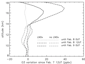
esti-mate the relative importance of dynamics and chemistry in the ozone evolution. This is shown in Fig. 6 for both the “reference” and the “no LNOx” simulations. As already
noticed in Fig. 1, Fig. 6 highlights the fact that the differ-ences between the “reference run” and the “no LNOx run”
mainly appear below 14 km. Above 14 km, there is nearly the same ozone variation, indicating that the NOxproduced
by lightning do not play a significant role above 14 km at the timescale of the simulation.
In Fig. 6, it should be noted that any absolute varia-tion of ozone between 7 February 12:00 UT and 8 February 00:00 UT is less than 4 ppbv. This value is much smaller than the variation that occurs later in the simulation. This is logi-cal since we have shown that the initial mean profile of ozone in Grid 2 was very close to the one computed 12 h later.
For the O3 variation, until 8 February 12:00 UT and 9
February 00:00 UT, there is a maximum at 16 km, which is 4 km higher than the maximum of chemical ozone
produc-Fig. 6. Mean of the ozone variation in the altitude range (8 km;
18 km) computed by RAMS in Grid 2 8 February 00:00 UT, 8 February 12:00 UT, 9 February 00:00 UT. The results including LNOxare presented using thick lines, and the results without LNOx
are shown using thin lines.
tion. Furthermore, at any time, the value of maximum ozone variation at 16–17 km altitude is much higher than the value of maximum ozone production at 12 km (see Fig. 5). Until 8 February 12:00 UT the variation has a maximum reaching 17 ppbv while the maximum of accumulated chemical ozone production reaches 4 ppbv at 12 km for the “reference” run. Later, for 9 February 00:00 UT, a ratio of ∼3 appears be-tween the maximum of ozone variation of (approximately 40 ppbv at 17 km), and the maximum of accumulated chem-ical ozone production (12 ppbv at 12 km).
It is possible that the ozone produced by chemistry below the TTL contributes to the ozone budget in the TTL if trans-ported by dynamical processes. But this contribution cannot be more than the ratio between the maximum of O3
produc-tion and the maximum of O3variation, (∼30%). This value
would be reached if all the O3 chemically produced below
13 km would enter the TTL.
In the next section the ozone budget is calculated in order to estimate the contributions of chemistry and dynamics to the ozone mixing ratio in the TTL.
5 Ozone budget in the TTL
In this section we focus on the tropical transitional layer, defined in this study as the layer between 13 km and the tropopause (∼17 km) as justified in Sect. 2.2. The budget is calculated between 8 February 00:00 UT and 9 February 00:00 UT in the domain defined horizontally by the bound-aries of Grid 2, and vertically by the 13 km and 17 km levels. In order to quantify the dynamical effect of deep convection in the TTL ozone budget, the same calculation was made over the most active period of convection, that is between 8
Grid 2
z = 17 km 30 km 13 kmE
w
N
S
z
Fig. 7. Schematic of the box used to calculate the ozone budget
in the TTL (shaded domain delimited at the bottom by the 13 km level, at the top by the 17 km level and on the sides by the boundary of Grid 2. The net contribution (inflowing flux or outflowing flux) on the budget for each side of the domain is indicated by the sense of the corresponding bold arrows.
February at 16:00 UT until 9 February at 00:00 UT. We are aware that the flux at 17 km is not an exact calculation of the stratosphere troposphere exchange (or STE, see Holton et al., 1995) because the altitude of the tropopause is not constant with time and space, especially during convective events when waves generated by convection can disturb the tropopause height. However here we try to give a tendency of what could occur around the tropopause. The domain is illustrated in Fig. 7.
The O3fluxes are calculated every hour for each side of
the domain as follows:
Fs=10−6 100. kboltz Z Z S Pair(i, j, k) Tair(i, j, k)
n(i, j, k).V (i, j, k)O3(i, j, k) dS
(1)
where Fs (in molec/s) is the flux through the surface S of the
domain, kboltzis the Boltzmann constant, Pairand Tairare,
re-spectively, the pressure (in hPa) and the temperature (in K), O3is the ozone concentration (in molec cm−3), i, j and k are
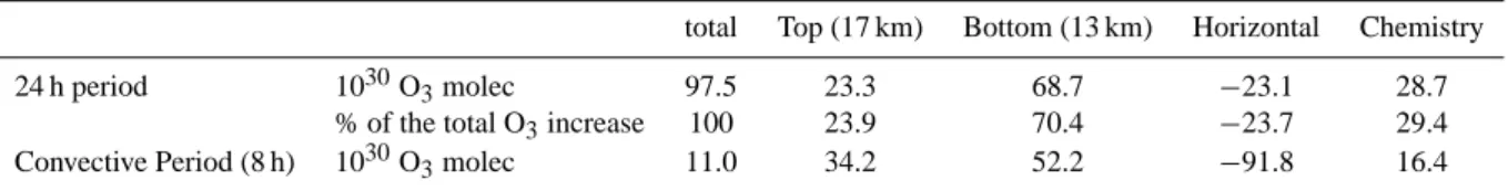
the usual indices for directions x, y, and z. n is the unit vec-tor perpendicular to the elementary surface dS, and V is the velocity vector. The sign of the flux is chosen to be positive when entering the TTL domain and negative when exiting it. Results of this calculation are shown in Fig. 8 and the 24 h integrated results are reported in Table 1. A 24 h period has been chosen in order to encompass a full ozone produc-tion/destruction diurnal cycle. Also provided in Table 1 is the same budget calculation results but for the 8 h period when convection is the most active. The total flux reported in Fig. 8 is the sum of the fluxes for each side of the domain plus the
Fig. 8. O3instantaneous fluxes on each side of the domain shown
in Fig. 7 between 8 February 00:00 UT and 9 February 00:00 UT for the “reference” run. The positive sign of the flux means that the flux is entering the domain. Also shown are the instantaneous O3chemical production within the domain for both simulations and the total of each flux including the O3production (solid line) for the
“reference” run.
net chemical ozone production (the net contribution of the ozone production and destruction terms) inside the domain for the “reference” run. The corresponding ozone produc-tion for the “no LNOx” run is also reported as an indication
but does not enter in the total flux calculation.
5.1 Total flux and horizontal flux
The total flux, is always positive, except between 19:00 UT and 22:00 UT. This explains why the O3concentration
gen-erally increases during this period, except around 20:00 UT as it was previously seen in Fig. 1 (see Sect. 2.3).
The horizontal flux is characterised by two different dy-namical regimes. The first regime, until 16:00 UT, depicts most of the time positive values of the flux. It is char-acterised by a maximum at 06:00 UT of 4×1027molec/s (which is the maximum of all the fluxes considered until 16:00 UT), followed by an almost constant value slightly be-low 2×1027molec/s until 14:00 UT. The second regime is characterized by a decrease of the flux, leading to negative minimum value of −8×1027molec/s at 22:00 UT (which is also the absolute minimum of all the fluxes considered). The horizontal flux increases again after 22:00 UT but is still neg-ative. This change of dynamical regime, correlated to the high convective activity, is explained by two mechanisms. Firstly the change of direction of the wind in the western part of grid 2. In the TTL altitude range, there is a negative ozone gradient from south to north. During the first period of the considered 24 h period, the winds were mostly along the western edge of Grid 2 (northward direction), while during the second period, the winds on this side of the domain turn
Table 1. Integrated number of molecules of ozone entering the domain drawn in Fig. 7 during a 24 h period starting from 8 February
2001 00:00 UT, and during the 8 h convective period starting from 8 February 2001 16:00 UT (in 1030molec) for the “reference” run. The horizontal, the top, bottom and the chemical contributions are reported. A positive value means a gain for the domain. Also shown are the percentage contributions to the ozone molecule increase for the 24 h period.
total Top (17 km) Bottom (13 km) Horizontal Chemistry 24 h period 1030O3molec 97.5 23.3 68.7 −23.1 28.7
% of the total O3increase 100 23.9 70.4 −23.7 29.4
Convective Period (8 h) 1030O3molec 11.0 34.2 52.2 −91.8 16.4
to the north-west direction, increasing the ozone flow out of the grid. Secondly, the increase of the convection activity leads to an increase of the vertical fluxes of ozone as it will be shown in the next sub-sections. For mass conservation reasons below the tropopause where air masses cannot rise anymore, the vertical motion turn to horizontal motions, so that the horizontal motions increase in the TTL with an in-creasing convective activity. It is noted that the total flux follows roughly the time evolution of the horizontal flux, due to its relatively large values and variability compared to the other fluxes. However, when integrated on a 24 pe-riod (see Table 1), the contribution of the horizontal flux rep-resents only −23% of the total ozone increase (this means a net contribution of 23% ozone loss) due to the fact that most of the time, the vertical fluxes are anti-correlated with the horizontal flux and partially compensate them. Further-more, the large minimum of the second dynamical regime (from 16:00 UT) compensates the positive values of the first regime (before 16:00 UT). Integrated on the 8 h of the se-vere convective period, there is a net exiting horizontal flux of 91.8×1030 O3molecules while it is 4 times less then for
the 24 h calculation. Despite the large negative horizontal flux on the 8 h period, the total flux remains positive during this period but 9 times smaller (11×1030O
3molecules) than
for the 24 h period (97.5×1030 O3molecules). The positive
value is reached because, during the 8 h period, the vertical fluxes are large and positive and the chemistry contribution is significant, even if twice smaller than for the 24 h period. It is important to note that O3molecules entering or exiting
horizontally the flux calculation domain shown in Fig. 7 do not represent a loss or a gain for the TTL since most of the O3molecules exiting the domain horizontally will remain in
the TTL. The real gain or loss of O3molecules for the TTL
will be generated by the vertical fluxes or the O3chemical
production/destruction. These contributions are discussed in the next sub-sections.
5.2 Vertical flux at the bottom of the TTL
The vertical flux at 13 km is expected to give an important indication of how O3 chemically produced below the TTL
(see Figs. 5 and 6) can be transported into the TTL. This
flux oscillates around a zero value until 16:00 UT with a relatively weak magnitude compared to the horizontal flux. From this time its contribution is always positive and be-comes the largest source of ozone except during the two last hours. This is once again correlated with the convective ac-tivity in the simulation which is very intense during this pe-riod. From 16:00 UT, beginning time of the intense convec-tive period, an anti-correlation between the bottom flux and the horizontal flux is found. This result is consistent with the mass conservation principle. The mass conservation im-plies that the divergence of the wind is close to zero (it is perfectly zero if the incompressibility of the air is assumed). Then the net upward motion at a given location must be com-pensated by an increasing horizontal motion. This is true because the tropopause acts as a dynamical barrier (even if partially permeable), so that the flow cannot rise above and becomes mostly horizontal below the tropopause. As a con-sequence, an increasing upward motion at the bottom of the TTL increases the horizontal flow inside the TTL, generating a horizontal outflow of ozone.
As deduced from Table 1, the overall contribution of the flux at the bottom of the TTL is 70% of the total ozone in-crease for this 24 h period. This high ratio is logical consider-ing that this flux is almost all the time positive, or very weak when negative, during the 24 h period, while the other fluxes have a succession of negative and positive values, which weakens their contribution in the total ozone increase. For the 8 h of the intense convective period, the vertical flux at the bottom of the TTL corresponds to 52.2×1030O3molecules
entering the TTL. This is 76% of the same flux calculated for the 24 h period. This means that the main process re-sponsible for the large vertical flux value at 13 km in the 24 h calculation is deep convection.
In order to estimate the contribution of the chemistry in this upward O3flux, we have compared the bottom flux for
the “reference” run and the “no LNOx” run for the same 24
hour period. The calculation of the flux for the “no LNOx”
simulation provides values that are close to those of the “ref-erence” run, with differences that are generally not signif-icant. The basic explanation is the following. The “refer-ence” run and the “no LNOx” run have the same
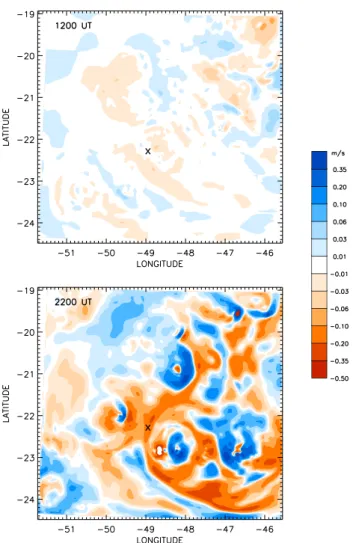
Fig. 9. Horizontal cross section at 17 km of the vertical velocity in
Grid 2 at 12:00 UT (upper panel) and 22:00 UT (lower panel). The location of Bauru is indicated by a cross.
vicinity of each convective cell in order to balance the con-vective updrafts. In the “reference” run, the ozone level at 13 km is higher than for the “no LNOx” run. As a
conse-quence, for the “reference” run, the magnitude of the ozone flux both in the updrafts and in the downdraft is large, and each contribution partially balance each other. Concurrently, the magnitude of the ozone flux both in the updrafts and in the downdraft is smaller for the “no LNOx” run, also leading
to a balance between the upward flux and the downward flux. The consequence is that the net vertical fluxes at 13 km (the sum of the contributions of the upward and downward fluxes) are comparable for the “reference” run and the “no LNOx”
run. The only significant difference between the two simula-tions appear from 22:00 UT (corresponding to the maximum intensity of the convective system) when the flux for the “ref-erence” simulation is ∼35% higher than for the “no LNOx”
simulation. When integrated on the 24 h period, the 13 km flux for the “reference” run is only 4% higher than for the “no LNOx” run. For the 8 h severe convective period, the same
calculation leads to a flux 11% higher for the “reference” run than for the “no LNOx” run. This tends to show the role of
convection in bringing O3produced by LNOxbelow and at
the bottom of the TTL into the TTL.
The contribution of the flux at the bottom of the TTL could possibly be more important if the simulation was continued for a longer period since this could allow ozone chemically produced by LNOxat 12 km to be continuously transported
into the TTL, or the LNOx produced at 12 km to be
trans-ported during the night to 13 km, where O3can be produced
chemically after sunrise.
5.3 Vertical flux close to the tropopause
As mentioned earlier in this section, the top flux does not il-lustrate directly the role of STE in this TTL ozone budget. It can however give an indication of what is happening in the tropopause region. This contribution is negative between 05:00 UT and 20:00 UT, but its 24 h integrated value is posi-tive, corresponding to 24% of the total ozone increase. This value is relatively small compared to the 13 km flux in Ta-ble 1, but not negligiTa-ble and this contribution is high between 22:00 (8 February) and 00:00 UT (9 February) with values higher than 4×1027 molec/s at 2300 UT, which is higher than the 13 km flux values. Integrated during the 8 h of in-tense convection, the top flux contribution is 34.2×1030 O3
molecules while it is 23.3×1030 O3 molecules for the 24 h
period. As for the vertical flux at the bottom of the TTL, this latter result shows that the 24 h tendency for the top vertical flux is mostly explained by processes related to the convec-tive activity. In particular, it is worth noting that the sharp increase of 17 km downward ozone flux is correlated with an increase of the wave activity in the tropopause region, as il-lustrated in Fig. 9. This figure provides the vertical velocity at 17 km (thus close to the tropopause level) for 12:00 UT and 22:00 UT. For both times, a wave activity exists in the simu-lation, as shown by an alternation of upward and downward motions inside Grid 2, centred on places where the convec-tion is the most intense. It also shows that the vertical mo-tions are much stronger for 22 00:UT than for 12:00 UT. This is related to deep convection activity which generated grav-ity waves at the tropopause. Convection generated-waves are known to be isentropic. This means that the waves oscillate on iso-θ surfaces. However if these waves break, the motion is not isentropic anymore and air can cross iso-θ surfaces. These breaking waves potentially bring stratospheric ozone down to the upper troposphere. In the latter case we talk of stratosphere to troposphere transport (or STT), according to the nomenclature of Stohl et al. (2003). Two cases are possible for our simulation. Either the waves oscillate on iso-θ surfaces and on average, should not contribute to the ozone budget (the amount that crosses down the 17 km sur-face would cross up the same sursur-face a half period of the wave later, so that the average budget is zero), or the waves break, an thus the average vertical transport is not zero,
leading to STE. A full study with higher vertical resolution would be necessary to quantitatively estimate the STE and to conclude about the interpretation of the 17 km flux given here. However, in the present simulations there are several convective cells developing close in time and space. Thus there are several sources of waves. This is illustrated in the bottom panel of Fig. 9 where two waves develop around two convective cells located at 49.8◦E 22◦S, and 48◦E 22.5◦S which can interact and provoke perturbations. These per-turbations favour wave breaking (Albert Hertzog, personnal communication). Furthermore the increase of the top flux between 19:00 UT and 23:00 UT is relatively long compared to the quarter of the period of the wave. This period is gen-erally of a few hours. If this hypothesis is confirmed, our result would be compatible with the conclusions of Wang et al. (1995). Performing a 2-dimensional model simulation of the ozone redistribution by a convective storm in the Pacific Ocean, they have shown that the stratospheric ozone had a significant contribution to the composition of the upper tro-posphere. Olsen et al. (2002) using total column ozone ob-servations and potential vorticity field analysis, reached the same conclusion. Finally, it was shown in the simulations of Tulet et al. (2002), using a model similar to ours and with a coarser vertical resolution (700 m), that mid-latitude convec-tive systems can induce the intrusion of stratospheric ozone into the upper troposphere.
The increase of the contribution for both vertical fluxes (13 km and 17 km) during the convective activity might ex-plain the features observed in Fig. 2 for the latest variability profiles. In this figure (Cf. Sect. 2.3), two local maxima of ozone variability at the bottom and the top of the TTL are computed by the model. The increase of the vertical fluxes at the bottom and the top of the TTL is likely to increase the variability of ozone.
5.4 Chemical production inside the TTL
The contribution of the chemical ozone production inside the TTL for both simulations is also shown in Fig. 8. For the “reference” run, the maximum of this contribu-tion (∼1.5×1027molec/s) is relatively weak compared to the other contributions, but when integrated over 24 h, it repre-sents 29.4% of the total ozone increase. The ozone chemical production is zero during night-time, increases after sunrise and remains constant until 16:00 UT. From this time, which corresponds to the beginning of the intense period of con-vection, the ozone increases again, due to the fact that ozone precursors are lifted up to the TTL by deep convection and that LNOxis produced. A detailed analysis shows that the
main source term of chemical production is the NO2
photol-ysis, as explained in Sect. 4. During the convective period with sunlight (until ∼22:00 UT), it was shown that the raw ozone destruction term is 40% to 90% of the raw ozone pro-duction term so that the net chemical ozone propro-duction is positive. This percentage depends on the location with
re-spect to the convective cells. During the most intense period of convection (around 22:00 UT), it is worth noting that the contribution of the ozone production is negative. This is be-cause this period also coincides with sunset, and the ozone amount around 13–14 km at this time is comparable with the amount of NOx. Thus, ozone is destroyed by NOx at
sun-set, because of O3titration. The maximum of convection, if
shifted in time with respect to sunset, would have increased the contribution of chemical production in the TTL ozone budget. Integrated over the 8 h period of severe convection, the number of ozone molecules produced in the domain of calculation is roughly half (57%) the number of molecules produced during the 24 h period. This is due to the fact that the 8 h period encompasses the ozone destruction at sunset but also the period between 18:00 UT and 20:00 UT when the ozone production is maximum. This number of 16.4×1030 O3molecules produced in the domain during the 8 h period
is relatively small compared to the dynamical fluxes during the same period. However, keeping in mind that the sum of the dynamical fluxes is slightly negative, this ozone produc-tion ensures the ozone budget to be positive during the severe convective period.
For the “no LNOx” simulation, the behaviour is
qualita-tively comparable with the results of the “reference” run, but the production of ozone is quantitatively much less. For the 24 h integration period, the O3 production inside the TTL
without LNOxrepresents 29% of the ozone production with
LNOx. This result stresses the local role of LNOxin
pro-ducing ozone directly inside the TTL, even if the maximum of ozone LNOx production is below the TTL, as shown in
Fig. 5. The role of LNOxin producing ozone inside the TTL
is emphasized during the intense period of convection. From Subsects. 5.2 and 5.4 it can be concluded that, from the point of view of the ozone increase in the TTL, light-ning produced NOxplay a more important role in producing
locally ozone than in producing ozone below the TTL that would be vertically transported later up to the TTL.
5.5 Budget summary
As a consequence of the time evolution of each contribution in the TTL ozone budget, the ozone evolution in the TTL can be explained by the sum of each contribution. Between 8 February at 00:00 UT and 09:00 UT, the ozone amount in the TTL increases, mainly due to the horizontal flux. After that, until 14:00 UT, the increase is due both to the horizontal flux and the chemical ozone production. Before the horizontal flux becomes negative, the ozone increase is due to both the chemical production and the vertical bottom flux, as a conse-quence of the strong convective activity. Between 19:00 UT and 22:00 UT when the total flux is negative, the high contri-bution of the bottom and tropopause fluxes partially compen-sate the large minimum of the horizontal flux. From 22:00 on 8 February to 00:00 on 9 February, the ozone increase is due to the vertical fluxes at the bottom and the top of the TTL.
To summarise, this section shows that the behaviour of ozone in the TTL during the period of convection is mainly due to the dynamics, the chemistry being responsible for
∼29%. This contribution could have been higher for cases with intense convection out of the sunset period. The vertical dynamics, especially at the end of the period of calculation, is strongly related to deep convection: atmospheric waves generated at the top of the convection might favour the pene-tration of higher amounts of stratospheric ozone down to the TTL, and vertical flux at the bottom of the TTL plays the major role in the budget since it represents 70% of the total ozone increase over the 24 h period of the budget calculation, since this contribution is almost always positive. The correla-tion between the chemical ozone produccorrela-tion inside the TTL and the convection activity is also highlighted in this budget. Calculating the same budget for the 8 most active hours of convection shows the importance of the vertical fluxes during this period since the total number of ozone molecules enter-ing the TTL vertically durenter-ing the 8 h period is comparable to the same number calculated for the 24 h period. The results have shown that there are two different chemical and dynam-ical regimes that have an impact the ozone budget: before and during the convective period. The large negative contri-bution of the horizontal flux, balanced by the vertical ozone flux, is explained by the conservation of mass.
6 Conclusion and perspectives
Because the upper troposphere is a key region for the atmo-spheric chemistry, especially in the tropics where chemical exchanges between the troposphere and the stratosphere are known to occur, a large number of studies have documented this issue since a decade. Among them, the study of the impact of deep convection on the upper troposphere com-position is one important aspect of this issue. This needs to be investigated using measurements or/and modelling ap-proach, at different scales of time and space, and in different regions (oceanic or continental). Most of the modelling stud-ies on this aspect investigated the cloud scale approach (e.g. Yin et al., 2001; DeCaria et al., 2005) or the large scale ap-proach (Labrador et al., 2004). Here we focus on the study of the ozone behaviour in the upper troposphere, and partic-ularly in the tropopause transitional layer (TTL), for an un-published type of convective system: an extreme continen-tal non-organised convective cluster. We have performed the simulation of the event which occurred on 8 February 2001 in Brazil, using a mesoscale model with on-line chemistry. The companion paper (Part 1: Mar´ecal et al., 2006) focussed on the meteorological simulation and on the ozone precursor results. They showed the average importance of deep con-vection in the vertical transport of ozone precursors from the surface to between 10 and 15 km altitude. They also showed the importance of lightning produced NOxin the chemistry
of other ozone precursors in the upper troposphere, between 8 and 15 km.
We can summarise the main results of the second part of this series of papers as follows. During the severe convective event, the disturbed layer of ozone in the TTL simulated by the model qualitatively and quantitatively reproduces the set of DMI O3sonde observations from Bauru during the 2004
wet season. On average, an inflection around 15 km in the ozone vertical profile is reproduced. Qualitatively, the vari-ability of the ozone in the fine grid of the simulation is com-parable with the ozone sonde observations: a relatively high variability in the TTL and a much lower variability above the tropopause. A budget of ozone in the TTL was calcu-lated during 24 h including the time of the convective event. Firstly, it should be stressed that during the most intense pe-riod of the convection, a strong signature of the convective activity was detected in the vertical flux at 13 km, in the downward motions around the tropopause and in the ozone chemical production inside the TTL. Secondly, this 24 h bud-get shows that this increase of ozone in the TTL with respect to the initial state is mainly due to the dynamics, but with a significant contribution of the chemistry. In this case study, the major contribution in the budget is the vertical flux at the bottom of the TTL which accounts for 70% of the total O3
increase because this contribution is almost always positive during the 24 h period or close to zero when negative. This contribution increases with the convection activity. A part of this 70% is due to chemical production of ozone below the TTL which is transported higher in the TTL by deep con-vection. The chemical production of ozone within the TTL is smaller but still significant since it represents 29% of the ozone budget. Finally we have found that stratosphere to troposphere transport associated with convection-generated gravity wave breaking can occur. A complete high resolu-tion study is needed to exactly quantify this contriburesolu-tion. In the present case, chemical production plays a weaker role than the dynamics in the TTL O3distribution. One of the
ex-planations is that the maximum of the chemical production occurs at 12 km, on average, and is thus below the bottom of the TTL. A significantly longer simulation might change this ratio since it could allow the ozone chemically produced around 12 km to be transported into the TTL by the large scale ascent. It could also allow the LNOx produced
dur-ing the night below the TTL to be transported up to 13 km, where O3can be produced after sunrise. It could also allow
the LNOx produced above 13 km to form ozone after
sun-rise. However, a longer simulation would lead to a different type of study, since it would imply a larger domain of simu-lation. In our simulation results, the chemical production of ozone is mainly due to the presence of LNOx in the upper
troposphere even though it was shown that ozone precursors other than LNOxalso contributed to this chemical
produc-tion. Comparison of simulation results with or without the parameterisation of LNOx shows that the ozone production
is enhanced by a factor of 4 when the lightning parameteri-sation is switched on.
This study shows that a mesoscale model with on-line chemistry is a powerful tool to study the chemistry in relation with deep convection: it can explicitly resolve the convec-tion, and can take into account a relatively large area around the event studied. Direct measurements to compare with model outputs are needed to better estimate the quality of the modelling results. This will be done in the future by studying events from the HIBISCUS/Troccinox/Troccibras 2004 field campaign, from which we can obtain information on H2O,
O3, CO, NOx, and halogen VSLS. The chemistry of halogen
species will then be included in the model, as well as the full set of chemical reactions involving Oxcompounds to better
constrain the chemistry in the stratosphere. Another study of a convective system in the same area will determine if the O3
behaviour computed here can be reproduced.
Acknowledgements. This modelling study is supported by funds
from the 5t h PCRD (HIBISCUS project) and the French Centre National de le Recherche Scientifique (Programme National de Chimie Atmosph´erique). This work makes use of the RAMS model, which was developed under the support of the National Science Foundation (NSF) and the Army Research Office (ARO). Computer resources were provided by CINES (Centre Informatique National de l’Enseignement Sup´erieur), project pce2227. The authors thank V.-H. Peuch from M´et´eo France for providing the MOCAGE fields that were used to initialise the chemistry model. G. Foret from LaMP is also thanked for helping with the use of the chemistry model. We are grateful to Albert Hertzog at Laboratoire de M´et´eorologie Dynamique, Palaiseau, for his comments about gravity waves generated by convection.
Edited by: M. G. Lawrence
References
Aumont, B., Jaecker-Voirol, A., Martin B., and Toupance, G.: Tests of some reduction hypotheses made in photochemical mecha-nisms, Atmos. Env., 30, 2061–2077, 1996.
Barth, M. C., Sillman, S., Hudman, R., Jacobson, M. Z., Kim, C.-H., Monod, A., and Liang, J.: Summary of the cloud chemistry modelling intercomparison: Photochemical box model simulation, J. Geophys. Res., 108(D7), 4214, doi:10.1029/2002JD002673, 2003.
Brewer, A. M.: Evidence for a world circulation provided by mea-surements and vater vapour distributions in the stratosphere, Q. J. R. Meteorol. Soc., 75, 351–363, 1949.
Cotton, W. R., Pielke Sr., R. A., Walko, R. L., Liston, G. E., Tremback, C. J., Jiang, H., McAnelly, R. L., Harrington, J.-Y., Nicholls, M. E., Carrio, G. G., and McFadden, J. P.: RAMS 2001: Current status and future directions, Meteorol. Atmos. Phys., 82, 5–29, doi:10.1007/s00703-001-0584-9, 2003. DeCaria, A. J., Pickering, K. E., Stenchikov, G. L. and Ott,
L. E.: Lightning-generated NOx and its impact on tropo-spheric ozone production: A three-dimensional modelling study of a Stratosphere-troposphere experiment: radiation, aerosols and ozone (STERAO-A) thurderstorm, J. Geophys. Res., 110, D14303, doi:10.1029/2004JD005556, 2005.
Dessler, A. E.: The effect of deep, tropical convection on the tropical tropopause layer, J. Geophys. Res., 107(D3), 4033, doi:10.1029/2001JD000511, 2002.
Dickerson, R. R., Huffman, G. J., Luke, W. T., Nunnermacker, L.J., Pickering, K. E., Leslie, A. C. D., Lindsey, C. G., Slinn, W. G. N., Kelly, T.J., Daum, P. H., Delany, A. C., Greenberg, J. P., Zimmerman, P. R., Boatman, J. F., Ray, J. D., and Stedman, D. H.: Thunderstorms: an important mechanism in the transport of air pollutants, Science, 235, 460–465, 1987.
Folkins, I., Braun, C., Thompson, A. M., and Witte, J.: Tropi-cal ozone as an indicator of deep convection, J. Geophys. Res., 107(D13), doi:10.1029/2001JD001178, 2002.
Gr´egoire, P. J., Chaumerliac, N., and Nickerson, E. C.: Impact of Cloud Dynamics on Tropospheric Chemistry: Advances in Mod-eling the Interactions Between Microphysical and Chemical Pro-cesses, J. Atmos. Chem., 18 , 3 , 247–266, 1994.
Holton, J. R., Haynes, P. H., McIntyre, M. E., Douglass, A. R,. Rood, R. B., and Pfister, L.: Stratosphere-Troposphere exchange, Rev. Geophys, 33, 403–439, 1995.
Jourdain, L.: Mod´elisation des oxydes d’azote et de l’ozone dans le mod`ele de circulation g´en´erale LMDzT-INCA : rˆole des ´emissions par les ´eclairs et par l’aviation subsonique, Ph.D. The-sis, Universit´e Paris 6, July 4th, 2003.
Komhyr, W. D., Barnes, R. A., Brothers, G. B., Lathrop, J. A., and Opperman, D. P: Electrochemical concentration cell ozonesonde performance evaluation during STOIC 1989, J. Geophys. Res., 100, 9131–9244, 1995.
Labrador, L. J., von Kuhlmann, R., and Lawrence, M. G.: Strong sensitivity of the global mean OH concentration and the tropo-spheric oxidizing efficiency to the source of NOxfrom lightning,
Geophys. Res. Lett., 31, L06102, doi:10.1029/2003GL019229, 2004.
Mar´ecal, V., Rivi`ere, E. D., Held, G., Cautenet, S., and Freitas, S.: Modelling study of the impact of deep convection on the UTLS air composition. Part 1: analysis of the ozone precursors, Atmos. Chem. Phys., 6, 1567–1584, 2006.
Olsen, M. A., Douglass, A. R., and Schoeberl, M. R.: Esti-mating the downward cross-tropopause ozone flux using col-umn ozone and potential vorticity, J. Geophys. Res, 107, 4636, doi:10.1029/2001JD002041, 2002.
Peuch V.-H., Amodei, M., Barthet, T., Cathala, M.-L., Josse, B., Mi-chou M., and Simon, P.: MOCAGE, MOd`ele de Chimie Atmo-sph´erique `a Grande Echelle, Proceedings of M´et´eo-France work-shop on atmospheric modelling, December 1999, 33–36, 1999. Pickering, K. E., Wang, Y., Tao, W.-K., Price, C., and M¨uller,
J.-F.: Vertical distributions of lightning NOxfor use in regional and
global chemical transport models, J. Geophys. Res., 103(D23), 31 203–31 216, 1998.
Pielke, R. A., Cotton, W. R., Walko, R. L., Tremback, C. J., Lyons, W. A., Grasso, L. D., Nicholls, M. E., Moran, M. D., Wesley, D. A., Lee T. J., and Copeland, J. H.: A comprehensive meteoro-logical modeling system – RAMS, Meteorol. Atmos., 49, 69–91, 1992.
Pundt, I., Pommereau, J.-P., Chipperfield, M. P., Van Roozen-dael, M., and Goutail, F.: Climatology of the stratospheric BrO vertical distribution by balloon-borne UV-Visible spectrometry, J. Geophys. Res., 107(D24), 4806, doi:10.1029/2002JD002230, 2002.
Ray, E. A., Moore, F. L., Elkins, J. W., Dutton, G. S., Fahey, D. W., V¨omel, H., Oltmans, S. J., Rosenlof, K. H.: Transport into the Northern Hemisphere lowermost stratosphere revealed by in situ tracer measurements, J. Geophys. Res., 104(D21), 26 565– 26 580, doi:10.1029/1999JD900323, 1999.
Ridley, B., Atlas, E., Selkirk, H., Pfister, L., Montzka, D., Walega, J., Donnelly, S., Stroud, V., Richard, E., Kelly, K., Tuck, A., Thompson, T., Reeves, J., Baumgardner, D., Rawlins, W. T., Mahomey, M., Herman, R., Friedl, R., Moore, F., Ray, E., and Elkins, J.: Convective transport of reactive constituents to the tropical and mid-latitude tropaupose region: I. Observations, At-mos. Environ., 38, 1259–1274, 2004.
Schoeberl, M. R.: Extratopical stratosphere-troposphere mass exchange, J. Geophys. Res., 109(D13), 303, doi:10.1029/2004JD004525, 2004.
Sherwood, S. C. and Dessler, A. E.: On the control of stratospheric humidity, Geophys. Res. Lett., 27, 2513—2516, 2000.
Stohl, A., Bonasoni, P., Cristofanelli, P., et al.: Stratosphere-troposphere exchange: A review, and what we have learned from STACCATO, J. Geophys. Res., 108(D12), 8516, doi:10.1029/2002JD002490, 2003.
Taghavi, M., Cautenet, S., and Foret, G.: Simulation of ozone pro-duction in a complex circulation region using nested grids, At-mos. Chem. Phys. 4, 825–838, 2004.
Taupin, F. G., Bessafi, M., Baldy, S., and Bremaud, P. J.: Tropo-spheric ozone above the southwestern Indian Ocean is strongly linked to dynamical conditions prevailing in the tropics, J. Geo-phys. Res., 104(D7), 8057–8066, doi:10.1029/98JD02456, 1999. Thompson, A. M., Witte, J. C., Oltmans, S. J., et al.: South-ern Hemisphere Additional Ozonesondes (SHADOZ) 1998– 2000 tropical ozone climatology 2. Tropospheric variability and the zonal wave-one, J. Geophys. Res., 108(D2), 8241, doi:10.1029/2002JD002241, 2003.
Thorntorn, D. C., Bandy, A. R., Blomquist, B. W., Bradshaw J. D., and Blake, D. R.: Verical transport of sulfur dioxide and dimethyl sulfide in deep convection and its role in new particle formation, J. Geophys. Res., 102, 28 501–28 509, 1997.
Tulet, P., Suhre, K., Mari, C., Solmon, F., and Rosset, R.: Mixing of boundary layer and upper tropospheric ozone during a deep con-vective event over Western Europe, Atmos. Environ., 36, 4491– 4501, 2002.
V¨omel, H., Oltmans, S. J., Johnson, B. J., Hasebe, F., Shiotani, M., Fujiwara, M,. Nishi, N., Agama, M., Cornejo, J., Paredes, F., and Enriquez, H.: Balloon-borne observations of water vapor and ozone in the tropical upper troposphere and lower stratosphere, J. Geophys. Res., 107(D14), doi:10.1029/2001JD000707, 2002. Wang, C., Crutzen, P. J., Ramanathan, V., and Williams, S. F.: The
role of a deep convective storm over tropical Pacific Ocean in the redistribution of atmospheric chemical species, J. Geophys. Res., 100(D6), 11 509–11 516, 1995.
Wang, C. and Prinn, R. G.: On the roles of deep convective clouds in tropospheric chemistry, J. Geophys. Res., 105, 22 269–22 297, 2000.
WMO (World Meteorological Organization), Scientific Assessment of Ozone Depletion: 2002, Global Ozone Research and Monitor-ing Project – Report, No. 47, Chapter 2: Very short-lived halogen and sulphur substances, 2.1–2.57, Geneva, 2003.
Yin, Y., Parker, D. J., and Carslaw, K. S.: Simulation of trace gas redistribution by convective clouds-Liquid phase processes, At-mos. Chem. Phys., 1, 19–36, 2001.