HAL Id: hal-00302596
https://hal.archives-ouvertes.fr/hal-00302596
Submitted on 3 May 2005
HAL is a multi-disciplinary open access
archive for the deposit and dissemination of
sci-entific research documents, whether they are
pub-lished or not. The documents may come from
teaching and research institutions in France or
abroad, or from public or private research centers.
L’archive ouverte pluridisciplinaire HAL, est
destinée au dépôt et à la diffusion de documents
scientifiques de niveau recherche, publiés ou non,
émanant des établissements d’enseignement et de
recherche français ou étrangers, des laboratoires
publics ou privés.
Streamflow dynamics at the Puget Sound, Washington:
application of a surrogate data method
N. She, D. Basketfield
To cite this version:
N. She, D. Basketfield. Streamflow dynamics at the Puget Sound, Washington: application of a
surrogate data method. Nonlinear Processes in Geophysics, European Geosciences Union (EGU),
2005, 12 (4), pp.461-469. �hal-00302596�
SRef-ID: 1607-7946/npg/2005-12-461 European Geosciences Union
© 2005 Author(s). This work is licensed under a Creative Commons License.
Nonlinear Processes
in Geophysics
Streamflow dynamics at the Puget Sound, Washington: application
of a surrogate data method
N. She and D. Basketfield
Seattle Public Utilities, City of Seattle, 700 5th Ave., Suite 4900, PO Box 34018, Seattle, WA 98124-4018, USA Received: 8 December 2004 – Revised: 4 February 2005 – Accepted: 23 March 2005 – Published: 3 May 2005 Part of Special Issue “Nonlinear deterministic dynamics in hydrologic systems: present activities and future challenges”
Abstract. Recent progress in nonlinear dynamic theory has
inspired hydrologists to apply innovative nonlinear time se-ries techniques to the analysis of streamflow data. However, regardless of the method employed to analyze streamflow data, the first step should be the identification of underlying dynamics using one or more methods that could distinguish between linear and nonlinear, deterministic and stochastic processes from data itself. In recent years a statistically rig-orous framework to test whether or not the examined time series is generated by a Gaussian (linear) process undergo-ing a possibly nonlinear static transform is provided by the method of surrogate data. The surrogate data, generated to represent the null hypothesis, are compared to the original data under a nonlinear discriminating statistic in order to re-ject or approve the null hypothesis. In recognition of this tendency, the method of “surrogate data” is applied herein to determine the underlying linear stochastic or nonlinear de-terministic nature of daily streamflow data observed from the central basin of Puget Sound, and as applicable, distin-guish between the static or dynamic nonlinearity of the data in question.
1 Introduction
Irregular patterns and spikes are common in streamflow data, and for decades hydrologists have been trying to explain the cause of irregularity in the streamflow. Various methods cov-ering a wide range of approaches, from detailed physically based computer models to complicated statistical analysis, has been used to characterize, analyze and forecast stream-flow dynamics. For example, shot noise stochastic models were used to generate spikes of streamflow (Weiss, 1977; Murrone et al., 1997), while a number of studies (Tong, 1990; Kantz and Schreiber, 1997; Schreiber and Schmitz, 2000) have shown that a linear stochastic process
undergo-Correspondence to: N. She
ing a possibly nonlinear static transform can also create very complex looking signals, suggesting that the apparent spikes and irregular patterns may be caused by either linear cor-relations or random input. Inspired by discoveries in the early 1980s of embedding theorems of time delay recon-struction (e.g. Packard et al., 1980; Takens, 1981) and of algorithms to calculate correlation dimensions of strange at-tractors (e.g. Grassberger and Procaccia, 1983a, b) numerous claims of low dimensional deterministic chaos in hydrologic time series data were reported (Nicolis and Nicolis,1984; Hense, 1987; Rodriguez-Iturbe et al., 1989; Jayawardena and Lai, 1994; Islam and Sivakumar, 2002; Sivakumar et al., 1999; Sivakumar, 2001; Sivakumar and Jayawardena, 2002; Regonda et al., 2004). But the results are not convinc-ing. As discussed by Kantz and Schreiber (1997), Hegger et al. (1999), and Schreiber and Schmitz (2000), when ap-plying algorithms developed to quantify deterministic low-dimensional chaos from field data, necessary procedures must be undertaken with care. These algorithms, especially the algorithms calculating correlation dimensions, only work under very strict conditions that data quality and quantity are sufficient to observe clear scaling regions. Further, these al-gorithms may incorrectly characterize non-chaotic and even linear stochastic process as low-dimensional chaos, particu-larly those of power law type linear correlations (e.g. Theiler, 1986; Osborne and Provenzale, 1989). Unfortunately, many early works in hydrology had not followed the necessary pre-cautions when these algorithms were applied to hydrologic data. Consequently, the initial results of the studies have been followed by a wave of corrections and counterclaims (Pasternack, 1999; Schertzer et al., 2002).
Before building a model for the data (e.g. for prediction purposes), or applying algorithms for phase-space recon-struction (e.g. calculating correlation dimensions), it is ad-visable to check whether the data alone suggest this type of modeling or calculation. Why use advanced nonlinear pre-diction models if there is no evidence of nonlinear struc-ture in the data? Or why put effort on detecting chaos from streamflow records at all if the pertaining data cannot be
462 N. She and D. Basketfield: Streamflow dynamics at the Puget Sound distinguished from linear stochastic process? The main
ob-jectives of the present study are to develop a statistically rig-orous, foolproof framework, called “surrogate data test”, to examine whether or not the streamflow time series is gen-erated by a Gaussian (linear) process undergoing a possi-bly nonlinear static transform, and to apply this procedure to characterize twenty-three selected daily streamflows from the central basin of Puget Sound in the state of Washington.
2 Surrogate data test
The surrogate data test herein is referred as a statistical pro-cedure that includes formulating a hypothesis, choosing a test statistic, specifying a probability of false rejection and gen-erating surrogate data sets from original data set. The sur-rogate data test has not been used to investigate underlying hydrologic dynamics until recent years though the compar-isons of surrogate data with original data were used in some hydrologic studies. Sivakumar et al. (1999) calculated corre-lation dimension from the original Singapore rainfall data to compare correlation dimension calculated from a surrogate of original data. No statistical test was really performed. Livina et al. (2003) compared seasonality of river flux in-crement series with the surrogate volatility series and found that the seasonal periodicity was almost diminished in sur-rogate volatility series, indicating that “periodic volatility” is a result of nonlinearity. Again, no test statistics were given. Moreover, the periodicity of surrogate volatility also disap-peared when the noise level increased. This scheme indicates that the surrogate volatility does not always diminish the seasonal periodicity of the volatility series, but rather elimi-nates the nonlinear part of the process which is proportional to the noise level. Laio et al. (2004) applied deterministic versus stochastic (DVS) plots to the decay phases of daily discharges of three rivers in Italy and detected nonlinearity from the data. DVS was first introduced by Casdagli (1991). Though it is robust towards non-Gaussianity, it is difficult to distinguish between a nonlinear non-Gaussian system with a linear Gaussian system, since the possible nonlinearities tend to be dominated by the stochastic component. Further-more, it is not a real statistical test “since no test statistics are produced which allows a unequivocal acceptance or re-jection of the null hypothesis of linearity” (Laio et al., 2004). Laio et al. (2004) also showed that a surrogate data set gen-erated from a linear decay system with non-Gaussian shot noise (see Eq. 3 below) appeared significantly different than an original data set and tested for reversibility using a sim-ple third order statistic. The authors concluded that when applying a surrogate data test, it is only valid to test a linear Gaussian stochastic process. It is apparent that the process generated from Eq. (3) is irreversible, but that does not mean that the process is not linear, so choosing a statistic in the surrogate data test is the key. Indeed, by choosing appro-priate robust nonlinear statistics, the surrogate data test may be justified when the noise deviates from a Gaussian process (Kantz and Schreiber, 1997; Schreiber and Schmitz, 2000).
We will show herein that the null hypothesis of linearity can not be rejected by our surrogate data test from Eq. (3), while the linearity is rejected correctly when we apply our surro-gate data test to a nonlinear system in Eq. (4). This indicates, when an appropriate statistic is chosen, surrogate data test is not only sensitive, but also robust and has larger statistical power. The surrogate data test, in any case, is a useful tool for data driven hydrologic analysis.
If the null hypothesis, that the underlying hydrologic pro-cess is a linear (possibly Gaussian) stochastic propro-cess, can not be rejected, then either it is due to the finite power of the test (we expect that the null hypothesis will be rejected only with probability β<1, where β is defined as the probability that the null hypothesis is rejected when it is indeed false) or the hypothesis actually describes the data properly. In the latter case, one can apply ARMA-type models to the hydro-logic data under investigation. If the null hypothesis is re-jected: (1) the rejection could have happened by chance with a probability of α, (2) the data may be nonstationary, (3) the measurement function could depend on more than one mea-surement and is noninvertible; or finally, (4) the process is nonlinear. In all cases but the last one the rejection is not jus-tified. One way to justify the rejection is to use other methods such as DVS plot to see whether or not the minimum pre-diction error occurs at smaller neighborhood size (Casdagli, 1991), or to compare the spectrum of increment series with surrogate volatility series (Linvina et al., 2003). After the rejection is justified, one may investigate other properties of the data or calculate additional invariants such as correlation or fractal dimensions.
The rest of this section is organized as follows: first we briefly introduce the procedures in the surrogate data test. Then we choose nonlinear statistics to test linear and non-linear decay systems with Poisson distributed shot noise (see Eqs. 3 and 4). Finally, we apply DVS plot to the nonlinear decay system to justify that the rejection of the null hypothe-sis is indeed due to existence of nonlinear properties.
The first step in the surrogate data test is to formulate a null hypothesis. In our case, the null hypothesis is that the streamflow data is sampled from a Gaussian linear stochastic process, i.e. qn = p X i=1 aiqn−i + q X j =1 bjηn−j, (1)
where qn is the subject time series, ηn is an independent
Gaussian random variable with zero mean and unit variance, and aiand bi are coefficients (Diggle, 1989).
Note that it is not our intention to merely test our hypothe-sis against one particular linear stochastic process, e.g. to test for the correct choice of a model of order p and q with spec-ified ai and bi. Rather, we wish to test against a whole class
of processes defined by Eq. (1) with unknown values p, q, ai
and bi. Moreover, we want to test the more general
x(t) 0 200 400 600 800 1000 0 500 1000 1500 (a) x(t) 0 200 400 600 800 1000 0 500 1000 1500 (b) time t x(t) 0 200 400 600 800 0 10 20 30 (c) time t x(t) 0 200 400 600 800 0 10 20 30 (d)
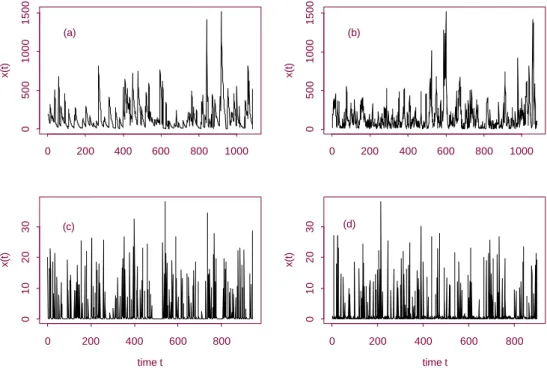
Figure 1. (a) Samples from a linear shot noise process defined in equation (3) and (b) a corresponding surrogate series (c) Samples from a nonlinear shot noise process defined in equation (4) and (d) a corresponding surrogate series
Fig. 1. (a) Samples from a linear shot noise process defined in Eq. (3)and (b) a corresponding surrogate series. (c) Samples from a nonlinear
shot noise process defined in Eq. (4) and (d) a corresponding surrogate series.
through the instantaneous, invertible and static, but possibly nonlinear functions given by
Qn =h(xn), xn = p X i=1 aiqn−i + q X j =1 bjηn−j (2)
where h is called measurement function, which may be non-linear and invertible. So, the process given by Eq. (2) is considered as a linear stochastic process defined in Eq. (1), but transformed by a possible static nonlinear measure-ment function h (Kantz and Schreiber, 1997; Schreiber and Schmitz, 2000).
Next, we need to choose a test statistic to actually per-form the test. Conventional statistics, like Student’s t or Chi-square in basic statistical analysis, result in a number that will lead us to either reject or accept the null hypothesis. From a statistical point of view, we hope the statistic cho-sen for the test is robust, i.e. when the distribution of sam-ples depart from assumed underlying distribution, the statis-tic still has test power. In order to test the hypothesis that the data is generated from the more general process defined in Eq. (2), a nonlinear test statistic λ must be computed from the data. This test statistic may be a prediction error or a dimension, but in any case it must not depend on the param-eters in Eq. (2), and also be robust and powerful enough to distinguish the difference between static and dynamic non-linearity.
The final step is to generate surrogate data sets. Recall that a linear stochastic process can be fully described by its first and second moments, such as its mean, variance and autocor-relation function, and also note that the unknown parameters in our null hypothesis reflect specific properties of interest of
the data. For example, the unknown autocorrelation coeffi-cients under a linear stochastic null hypothesis are reflected in the autocorrelation function of the data.
Now we apply the procedures described above to two ex-amples: one is a linear shot noise process, and the other is a nonlinear shot noise process. Both processes are, respec-tively, given by dx dt = −x(t ) + Np(t ) (3) dx dt = −x 2(t ) + N p(t ) , (4)
where Np(t )is the random driving process in the form of a
white Poisson noise and is defined by a sequence of pulses at random times τi, each pulse having an independent random
amplitude hi, i.e. Np(t ) = hi X i δ(t − τi) , (5)
where δ(·) is the Dirac delta function and {τi}come from a
Poisson distribution. Figure 1 shows the samples and their corresponding surrogate series generated from Eqs. (3) and (4).
Evidently, both samples are very different from their cor-responding surrogate series. To test the linearity versus non-linearity, we choose zeroth-order nonlinear prediction error as a discriminating statistic. It was shown that zeroth-order nonlinear prediction error is a robust and powerful statis-tic (Pikovsky, 1986; Kennel and Isabelle, 1992; Theiler and Prichard, 1996; Kantz and Schreiber, 1997).
464 N. She and D. Basketfield: Streamflow dynamics at the Puget Sound
Fig. 2. (a) Prediction errors for Eq. (3) and 19 corresponding
gates, (b) Prediction errors for Eq. (4) and 19 corresponding surro-gates,. Prediction errors are estimated using embedding dimension
m=1 and time delay τ =1.
The surrogate data test is set up in such a way that the null hypothesis may be rejected when the prediction error is smaller for the data than for all of the nineteen surrogates. Figure 2 shows the plots of the prediction errors. To distin-guish prediction errors between surrogates and original data we plot the prediction errors from surrogates on the left and the prediction errors from the original data on the right. As we can see from Fig. 2, the prediction error of the linear pro-cess is not significantly smaller than that of all nineteen sur-rogates, that is, the predictability is not significantly reduced by destroying possible nonlinear structure. The prediction error of the nonlinear process, however, is the smallest one among all nineteen surrogates. This shows that the test works correctly, even though the random errors are generated from a non-Gaussian process.
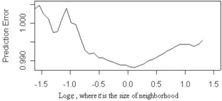
Further, we apply DVS plot to investigate whether or not the rejection is due to nonlinearity. Figure 3 shows clearly that the minimum prediction error occurs at medium neigh-borhood size, which is a signature of so called “weak non-linearity” when the nonlinear structure in the system is weak and the noise level is moderate (Casdagli, 1991).
3 Characterization of streamflow in central basin of Puget Sound
Puget Sound is a 35 000 km2region of western Washington located at the northwest corner of the United States. Cupped between the jagged Olympic Mountains to the west and the volcanic peaks of the Cascade Range to the east with majes-tic Mount Rainier standing at 4392 m, the Puget Sound basin has among the most diverse hydrologic conditions of any re-gion in the United States, varying from arid conditions in
Fig. 3. DVS plot for a nonlinear shot noise process defined in
Eq. (4). 1000 samples are generated from Eq. (4). Prediction er-rors are estimated using embedding dmension m=1 and time delay
τ=1.
the shadows of the Olympic and Cascade Mountains to very wet rainforest along the Pacific coast. In the coastal area and Cascade Mountains, the maximum precipitation occurs dur-ing the winter months, while in the eastern basins, with more steppe and continental climates, the maximum precipitation occurs in the early summer. On average, the region receives about 1000 mm of precipitation annually. Much of the an-nual precipitation falls between November and April as rain and with snow at high altitudes.
Streamflows in the Puget Sound basins are largely influ-enced by seasonal snowpack melt off over spring and early summer. Runoff from rainstorms and groundwater discharge (in the form of springs or seeps) from shallow aquifers also influence the amount and form of water that drives stream-flow in its rivers and streams. To better manage water re-sources in the Puget Sound basin, it is essential to have a clear understanding of the characteristics of streamflow hy-drology. Unlike the conventional characterization of stream-flow using either a physically based model or a statistically based model (such as regression analysis or ARMA), we use nonlinear dynamics tools developed for time series analysis to investigate the characteristics of the streamflow, such as dimensionality, predictability, periodicity, deterministic non-linearity and probability. The theoretical foundation of our characterization is borrowed from Taken’s time delay em-bedding theorem of phase-space reconstruction and surrogate data test described in the previous section.
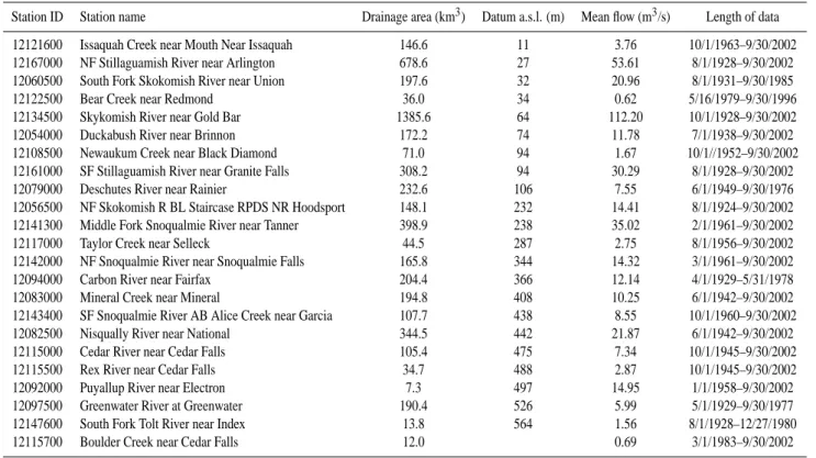
Twenty-three daily streamflow time series in central basin of Puget Sound are chosen for characterization. These streamflows represent three typical watersheds in Puget Sound basin: rainfall-driven streams, snowmelt-driven streams, and hybrid (mixed rainfall- and snowmelt-driven) streams. The drainage areas range from 12.2 to 1385.6 km2; average daily flows over the study time period (from 19.5 years to 74 years) range from 0.62 to 112.2 m3/s; the eleva-tions range from 11 to 564 m a.s.l.; and the length of the time series range from 20 to 74 continuous years. All stream-flow data are measured and processed by the United States Geologic Survey (USGS) and can be found at the website: http://waterdata.usgs.gov/nwis/sw. Table 1 lists some of the important physical characteristics of these twenty-three sub-basins and statistics of the observed streamflows.
Table 1. Physical characteristics of 23 streamflows in central Basin of Puget Sound.
Station ID Station name Drainage area (km3) Datum a.s.l. (m) Mean flow (m3/s) Length of data 12121600 Issaquah Creek near Mouth Near Issaquah 146.6 11 3.76 10/1/1963–9/30/2002 12167000 NF Stillaguamish River near Arlington 678.6 27 53.61 8/1/1928–9/30/2002 12060500 South Fork Skokomish River near Union 197.6 32 20.96 8/1/1931–9/30/1985 12122500 Bear Creek near Redmond 36.0 34 0.62 5/16/1979–9/30/1996 12134500 Skykomish River near Gold Bar 1385.6 64 112.20 10/1/1928–9/30/2002 12054000 Duckabush River near Brinnon 172.2 74 11.78 7/1/1938–9/30/2002 12108500 Newaukum Creek near Black Diamond 71.0 94 1.67 10/1//1952–9/30/2002 12161000 SF Stillaguamish River near Granite Falls 308.2 94 30.29 8/1/1928–9/30/2002 12079000 Deschutes River near Rainier 232.6 106 7.55 6/1/1949–9/30/1976 12056500 NF Skokomish R BL Staircase RPDS NR Hoodsport 148.1 232 14.41 8/1/1924–9/30/2002 12141300 Middle Fork Snoqualmie River near Tanner 398.9 238 35.02 2/1/1961–9/30/2002 12117000 Taylor Creek near Selleck 44.5 287 2.75 8/1/1956–9/30/2002 12142000 NF Snoqualmie River near Snoqualmie Falls 165.8 344 14.32 3/1/1961–9/30/2002 12094000 Carbon River near Fairfax 204.4 366 12.14 4/1/1929–5/31/1978 12083000 Mineral Creek near Mineral 194.8 408 10.25 6/1/1942–9/30/2002 12143400 SF Snoqualmie River AB Alice Creek near Garcia 107.7 438 8.55 10/1/1960–9/30/2002 12082500 Nisqually River near National 344.5 442 21.87 6/1/1942–9/30/2002 12115000 Cedar River near Cedar Falls 105.4 475 7.34 10/1/1945–9/30/2002 12115500 Rex River near Cedar Falls 34.7 488 2.87 10/1/1945–9/30/2002 12092000 Puyallup River near Electron 7.3 497 14.95 1/1/1958–9/30/2002 12097500 Greenwater River at Greenwater 190.4 526 5.99 5/1/1929–9/30/1977 12147600 South Fork Tolt River near Index 13.8 564 1.56 8/1/1928–12/27/1980 12115700 Boulder Creek near Cedar Falls 12.0 0.69 3/1/1983–9/30/2002
Table 2. Power spectrum analysis of 23 streamflows in central basin of Puget Sound.
Station ID Station name Dominate periodicity Harmonics Sub-harmonics 12054000 Duckabush River near Brinnon 6 months 12 months 12056500 NF Skokomish R BL Staircase RPDS NR Hoodsport 12 months 6 months
12060500 South Fork Skokomish River near Union 12 months 6 months 12079000 Deschutes River near Rainier 12 months 6 months
12082500 Nisqually River near National 6 months 12 and 82 months 12083000 Mineral Creek near Mineral 12 months 6 months
12092000 Puyallup River near Electron 6 months 12, 22 and 90 months 12094000 Carbon River near Fairfax 6 months 12 and 54 months 12097500 Greenwater River at Greenwater 12 months 3, 4 and 6 months 59 and 197 months 12108500 Newaukum Creek near Black Diamond 12 months 6 months 87 months 12115000 Cedar River near Cedar Falls 12 months 6 months
12115500 Rex River near Cedar Falls 12 months 6 months
12115700 Boulder Creek near Cedar Falls 12 months 6 months 40 months 12117000 Taylor Creek near Selleck 12 months 6 months 23 and 93 months 12121600 Issaquah Creek Near Mouth near Issaquah 12 months 6 months 25 and 95 months 12122500 Bear Creek near Redmond 12 months 30 months 12134500 Skykomish River near Gold Bar 6 months 12 months 12141300 Middle Fork Snoqualmie River near Tanner 6 months 12, 19 and 84 months 12142000 NF Snoqualmie River near Snoqualmie Falls 6 months 12, 25 and 84 months 12143400 SF Snoqualmie River AB Alice Creek near Garcia 6 months 12, 20 and 72 months 12147600 South Fork Tolt River near Index 6 months 12 months 12161000 SF Stillaguamish River near Granite Falls 12 months 6 months
466 N. She and D. Basketfield: Streamflow dynamics at the Puget Sound
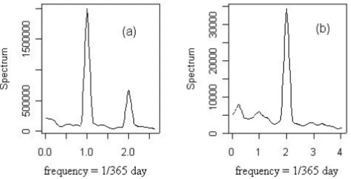
Fig. 4. Power spectrum analysis for streamfroms (a) at USGS
12167000 and (b) at USGS 12094000. (a) shows harmonic peri-odicity; (b) shows subharmonic periodicity.
Different streams with different drainage areas at different elevations respond differently to the winter inflow of mois-ture to the region. Streams at low elevations (e.g. USGS 12121600) tend to respond quickly and directly to the pre-cipitation that falls on the basin, since the basin tempera-tures are typically above freezing level, and all the precip-itation falls as rain. Streams at moderate elevations (e.g. USGS12115000) have a transient snow zone, where precip-itation frequently falls as snow but then melts a few days or weeks later in a cycle that is typically repeated many times in the winter. The transient snow zone can cause flooding if heavy rain and warm temperatures occur at the same time when snow has already accumulated. Typically streams of this type show a dual peaked hydrograph: one during the winter, another during spring or early summer. Figure 4a shows the power spectrum of streamflow at a moderate el-evation. Clearly, two periodicities occur at six-month and one-year periods. It can be seen that the annual periodicity is stronger than the six-month periodicity. This is referred to as harmonic cycles in time series analysis. However, Fig. 4b shows a different scenario, i.e. the six-month periodicity is stronger than the annual and long-term (54-month) periodic-ity. This is referred to as sub-harmonic in time series anal-ysis, which is usually the evidence of existing long term cy-cles.
Table 2 shows the results of power spectral analysis from which the periodicity of the streamflow time series are iden-tified clearly. Moreover, the complexity of the data is shown through the harmonics and sub-harmonics of frequencies and periodicity.
The deviation of hydrographs from typical dual peaks in some streamflows (most in moderate elevations) may be the effect of El Ni˜no Southern Oscillation (ENSO) phenomenon to transient snow zones. Numerous researchers (Koch et al., 1991; Redmond and Koch, 1991; Chiew et al., 1998) have shown that the snowpack in the Pacific Northwest regions is evidently affected by ENSO, such as Southern Oscilla-tion Index (SOI), sea surface temperatures (SST) and Pacific Decadal Oscillation (PDO). These oscillators usually have 3 to 10 year cycles. An El Ni˜no event can lead to a drier and warmer than normal winter, while a La Ni˜na event can
Fig. 5. DVS plots for two daily streamflow discharges in central
basin of Puget Sound (a) USGS 12097500, (b) USGS 12147600. Time delay and embedding dimensions are the same as in Table 3, where ε is the size of neighborhood.
lead to a wetter and cooler than normal winter. The vari-ability observed in the streamflows, both from year to year and within the year, is related to these large-scale features in the ocean and atmosphere. Correlations between stream-flows and ENSO have been found in many streams in Pacific Northwest (Peter et al., 2002; Piechota and Dracup, 1999). The streamflow records reflect the interactions between sea-sonality and long-term cycles of climate.
From Table 2, it is clear that either a six-month or a twelve-month periodicity dominates the streamflow dynam-ics. However, sub-harmonic frequencies are present in most data sets at moderate elevations. This implies that, not only annual and semi-annual cycles, but also long-term cycles play important roles in these streamflow processes. The in-teraction of a dominant frequency with harmonic and sub-harmonic frequencies may create various complex behav-iors of the streamflow from linear stochastic process to de-terministic chaos, or something in between such as quasi-periodicity or tori. Our next task, therefore, is to test these complexities using a surrogate data test.
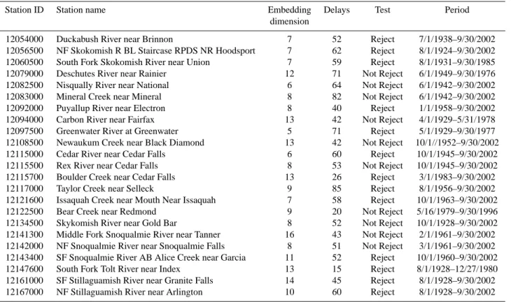
To conduct the surrogate data test, we need to choose an appropriate nonlinear statistic. As we demonstrated in the previous section, the zeroth-order prediction error is a ro-bust and powerful nonlinear statistic. Therefore, we use this statistic to test the twenty-three streamflows versus their cor-responding surrogates. If the null hypothesis were rejected, we use DVS plot for further investigation. The surrogate data test and the DVS plot are performed using the software pack-age TISEAN (Hegger et al., 1999).
The results of the surrogate data test for the twenty-three streamflows in the central basin of Puget Sound are presented in Table 3.
Zeroth-order prediction error is chosen as the test statis-tic. The time delay and embedding dimensions associated with prediction errors are the key elements in the algorithm of the zeorth-order prediction. If the time delay τ is taken too small, there is almost no difference between the different components of the embedding vectors, such that all points are concentrated around the diagonal. On the other hand, if it is taken too large, the different coordinates may be almost un-correlated, such that the reconstructed attractor becomes very
Table 3. Surrogate data tests of 23 streamflow in central basin of Puget Sound.
Station ID Station name Embedding Delays Test Period dimension
12054000 Duckabush River near Brinnon 7 52 Reject 7/1/1938–9/30/2002 12056500 NF Skokomish R BL Staircase RPDS NR Hoodsport 7 62 Reject 8/1/1924–9/30/2002 12060500 South Fork Skokomish River near Union 7 59 Reject 8/1/1931–9/30/1985 12079000 Deschutes River near Rainier 12 71 Not Reject 6/1/1949–9/30/1976 12082500 Nisqually River near National 6 64 Not Reject 6/1/1942–9/30/2002 12083000 Mineral Creek near Mineral 8 82 Not Reject 6/1/1942–9/30/2002 12092000 Puyallup River near Electron 8 40 Reject 1/1/1958–9/30/2002 12094000 Carbon River near Fairfax 13 42 Not Reject 4/1/1929–5/31/1978 12097500 Greenwater River at Greenwater 5 71 Reject 5/1/1929–9/30/1977 12108500 Newaukum Creek near Black Diamond 13 42 Not Reject 10/1//1952–9/30/2002 12115000 Cedar River near Cedar Falls 6 60 Reject 10/1/1945–9/30/2002 12115500 Rex River near Cedar Falls 8 53 Not Reject 10/1/1945–9/30/2002 12115700 Boulder Creek near Cedar Falls 13 26 Reject 3/1/1983–9/30/2002 12117000 Taylor Creek near Selleck 9 85 Reject 8/1/1956–9/30/2002 12121600 Issaquah Creek near Mouth Near Issaquah 7 58 Reject 10/1/1963–9/30/2002 12122500 Bear Creek near Redmond 9 20 Not Reject 5/16/1979–9/30/1996 12134500 Skykomish River near Gold Bar 8 52 Not Reject 10/1/1928–9/30/2002 12141300 Middle Fork Snoqualmie River near Tanner 16 43 Not Reject 2/1/1961–9/30/2002 12142000 NF Snoqualmie River near Snoqualmie Falls 8 51 Not Reject 3/1/1961–9/30/2002 12143400 SF Snoqualmie River AB Alice Creek near Garcia 11 52 Reject 10/1/1960–9/30/2002 12147600 South Fork Tolt River near Index 13 15 Reject 8/1/1928–12/27/1980 12161000 SF Stillaguamish River near Granite Falls 14 45 Reject 8/1/1928–9/30/2002 12167000 NF Stillaguamish River near Arlington 10 60 Reject 8/1/1928–9/30/2002
complicated and the original structure of the attractor is lost. The choice of time delay τ is here based on the so-called mu-tual information (Frazer and Swinney, 1986), which can be considered as a nonlinear analogue to linear correlation and is more adequate than an autocorrelation function when non-linear dependencies are present. A possible rule to choose an appropriate time delay τ is to use the first minimum of the time delayed mutual information . Thus, the components of the embedding vectors can be considered independent at least with this lag.
It can be seen that, for most streamflows in Table 3 the time delays are quite large, somewhere from 15 days to 85 days. This may be due to the fact that most streamflows in this study are either snowmelt-driven or hybrid (mixed rainfall-and snowmelt-driven). These sub-basins receive most pre-cipitation from November to April. During these six months, a cycle of snow falls and melts off (described earlier) oc-curs frequently. The snowpack at transient zones are typi-cally completely melted off in early June. During summer months (from July to September), these sub-basins receive very little precipitation. Therefore, streamflows in these sub-basins may have long-term persistence. Also, soil moisture and permeability, forest canopies, and topographies of sub-basins may be factors associated with the time delay. While no extensive investigation on the effects of time delay has been conducted on these streamflows, the study by Regonda et al. (2004) in a nearby area, Stillaguamish River, found a similar long time lag using the first zero autocorralation
function. The long time showed the additional complexity inherent in the subject streamflow.
The embedding dimensions are determined using false nearest neighbors proposed by Kennel et al. (1992). The range of embedding dimensions for these streamflows are from 5 to 16. Note that the embedding dimension thus ob-tained is not necessarily equal to the dimension of the entire hydrologic system. By Taken’s theorem, the original system is topologically equivalent to embedded system as long as the embedding dimension m is as twice as large than the di-mension of the original system n. Therefore, the embedding dimension is an upper bound of the real dimension of the system.
Using the surrogate data test, we find that about 57% of the selected streamflow data sets were unlikely to be gener-ated by linear stochastic processes. So, we further investi-gate, using DVS plot, whether or not the rejections were due to nonlinearity. Figure 5 shows plots of the prediction errors as a function of log neighborhood size from two streamflows measured at USGS 12097500 (Greenwater River at Green-water, WA) and USGS 12147600 (South Fork Tolt River Near Index, WA), respectively. From Fig. 5a, one can see that the minimum prediction error occurs at small neighborhood size, which is a clear indication of nonlinearity. However, in Fig. 5b, the minimum is not seen at small neighborhood size, but somewhere in the moderate neighborhood size. This shows that determinism is weaker, presumably due to a much higher noise level. Most DVS plots for streamflows are
468 N. She and D. Basketfield: Streamflow dynamics at the Puget Sound similar to Fig. 5b, which indicates that linear stochastic
pro-cesses and high dimensional deterministic propro-cesses make no difference in short-term prediction. For the rest of the 43% streamflows that did not pass the surrogate data test, it ap-pears that the data were generated from stochastic processes.
4 Conclusion and closing remarks
In this paper we introduced a statistically rigorous frame-work, called surrogate data test, to examine whether or not the streamflow under investigation is generated by a Gaus-sian (linear) process undergoing a possibly nonlinear static transform. The surrogate data, generated to represent the null hypothesis, are compared to the original data under a non-linear discriminating statistic in order to reject or accept the null hypothesis. The negative result can mean several things. The statistics chosen may just not have any power to detect the kind of nonlinearity present. Alternatively, the underly-ing process may be linear and the null hypothesis true. It could also be, and this seems the most likely option after all we know about the equations governing hydrologic process, which is nonlinear but the single time series at this sampling covers such a poor fraction of the rich dynamics that it must appear linear stochastic to the analysis. When the null hy-pothesis is rejected, we have to keep in mind that the rejec-tion has to be justified because it may depend on the applied nonlinear method and the choice of the nonlinear statistics (e.g. a linear process with Poisson distributed shot noise was incorrectly rejected by using a simple third order statistic, but was accepted by using prediction errors of false nearest neighbors, see Sect. 2), or the measurement function could depend on more than one measurement. Hence, we suggest to use more than one method such as DVS plot or to compare the spectrum of increment series with surrogate volatility se-ries to confirm the result. We have to also keep in mind that a rejection after the justification only indicates nonlinearity, not necessarily low dimensional deterministic chaos.
Streamflow is a complex hydrologic process. Even the knowledge that certain components of a hydrologic system may exhibit nonlinear behavior does not necessarily lead to the conclusion that a specific output of the system (e.g. streamflow) is consequently nonlinear, or that this nonlinear-ity will be proven evident in streamflow dynamics. Instead of pre-supposing the underlying dynamics, we use surrogate data test to represent the dynamics in an ‘inverse’ manner. We have shown in Sect. 2 that surrogate data test is a power-ful statistical tool that is capable of distinguishing nonlinear dynamics from linear stochastic processes, even if the noise is generated from non-Gaussian sources. This has significant implications in hydrology because in most cases streamflow records are obtained through a measurement function and their statistical distribution are usually unknown.
Unlike conventional characterization of streamflow, we introduced concepts fairly new and recent to hydrologists, such as embedding dimension, time lag and prediction er-rors. These concepts have significant application to
hydrol-ogy. Embedding dimension and time lag illustrate the com-plexity of the system. Prediction errors show certain struc-ture of the dynamic system. For example, embedding di-mension m gives an upper bound of the original dynamic system. Moreover, this bound is determined from measured data rather than through a prejudiced model subjectively se-lected by investigators. We applied these concepts together with surrogate data test to characterize twenty-three stream-flows in the central basin of Puget Sound. As we have shown in Sect. 3 that the complexity of these streamflows are char-acterized by the length of time delays, the degrees of em-bedding dimensions, harmonic and sub-harmonic periods in streamflow time series, and the linear stochastic and nonlin-ear dynamic processes presented in the streamflows.
In the review of searching for lower dimensional chaos from field data, we recommend researchers to use surrogate data test as the first cut of screening. If the nonlinearity does not exist in the data, why not bother to calculate invariants such as fractal and correlation dimensions to make a possi-ble false claim?
Acknowledgements. The authors would like to thank B. Sivakumar
for his comments on an earlier version of the manuscript.
Edited by: B. Sivakumar Reviewed by: two referees
References
Casdagli, M.: Chaos and deterministic versus stochastic nonlinear modeling, J. Roy. Stat. Soc. B, 54, 303–324, 1991.
Chiew, F. H. S., Piechota, T. C., Dracup, J. A., and McMahon, T. A.: El Ni˜no/Southern Oscillation and Australian rainfall, streamflow and drought: links and potential for forecasting, J. Hydrol., 204, 138–149, 1998.
Diggle, P. J.: Time Series A Biostatistical Introduction, Oxford Uni-versity Press, Oxford, 1989.
Frazer, A. M. and Swinney, H. L.: Independent coordinates in strange attractors from mutual information, Phys. Rev. (A), 33, 1134–1140, 1986.
Grassberger, P. and Procaccia, I.: Characterization of strange attrac-tors, Phys. Rev. Lett., 50, 346–349, 1983a.
Grassberger, P. and Procaccia, I.: Estimation of the Kolmogorov entropy from a chaotic signal, Phys. Rev. (A), 28, 2591–2593, 1983b.
Hegger, R., Kantz, H., and Schreiber, T.: Practical implementa-tion of nonlinear time series methods: The TISEAN package, CHAOS, 9, 413–435, 1999.
Hense, A.: On the possible existence of a strange attractor for the southern oscillation, Beitr. Phys. Atmos., 60, 34–47, 1987. Islam, M. N. and Sivakumar, B.: Characterization and prediction
of runoff dynamics: A nonlinear dynamical view, Adv. Wat. Re-sour., 25, 179–190, 2002.
Jayawardena, A. W. and Lai, F.: Analysis and prediction of chaos in rainfall and stream flow time series, J. Hydro., 153, 23–52, 1994. Kantz, H. and Schreiber, T.: Nonlinear Time Series Analysis,
Cam-bridge University Press, CamCam-bridge, 1997.
Kennel, M. B., Brown, R., and Abarbanel, H. D. I.: Determining embedding dimension for phase-space reconstruction using a ge-ometrical construction, Phys. Rev. (A), 45, 3403–3411, 1992.
Kennel, M. B. and Isabelle, S.: Method to distinguish possible chaos from colored noise and to determine embedding param-eters, Phys. Rev. (A), 46, 3111, 1992.
Koch, R. W., Buzzard, C. F., and Johnson, D. M.: Variation of snow water equivalent and streamflow in relation to the El Ni˜no/ South-ern Oscillation, Proceedings, WestSouth-ern Snow Conference, 59, 37– 48, 1991.
Laio F., Porporato, A., Ridolfi, L., and Rodriguez-Iturbe, I.: Mean first passage times of processes driven by white shot noise, Phys. Rev. (E), 63, 036105, 1–8, 2001.
Laio F., Porporato, A., Ridolfi, L., and Tamea, S.: Detecting non-linearity in time series driven by non-Gaussian noise: the case of river flows, Nonlin. Proc. Geophys, 11, 463–470, 2004,
SRef-ID: 1607-7946/npg/2004-11-463.
Linvina, V. N., Ashekenazy, Y., Braun, P., Monetti, R., Bunde, A., and Havlin S.: Nonlinear volatility of river flux flunctuations, Phys. Rev. (E), 67, 042101, 1–4, 2003.
Murrone, F., Rossi, F., and Claps, P.: Conceptually-based shot noise modeling of streamflows at short time intervals, Stoch. Hydrol. Hydrauli., 11, 483–510, 1997.
Nicolis, C. and Nicolis, C. G.: Is there a Climatic Attractor?, Na-ture, 311, 529–532, 1984.
Osborne, A. R. and Provenzale, A.: Finite correlation dimension for stochastic systems with power-law spectra, Physica D, 35, 357–381, 1989.
Packard, N. H., Crutchfield, J. P., Farmer, J. D., and Shaw, R. S.: Geometry from a time series, Phys. Rev. Lett., 45, 712–716, 1980.
Pasternack, G. B.: Does the river run wild? Assessing chaos in hydrologic systems, Adv. Wat. Resour., 23, 253–260, 1999. Peter, M. K., Jennifer, P. B., and Michael, C. F.: Climatic and
hydro-logic variability in a coastal watershed of southwestern British Columbia, JAWRA, 38, 1437–1449, 2002.
Piechota, T. C. and Dracup, J. A.: Long range streamflow fore-casting using El Ni˜no-Southern Oscillation Indicators, J. Hydrol. Engng., 4, 144–151, 1999.
Pikovsky, A.: Noise filtering in the discrete time dynamical sys-tems, Sov. J. Commun. Technol. Electron., 31, 911–914, 1986.
Redmond, K. T. and Koch, R. W.: Surface climate and streamflow variability in the western United States and their relationship to large-scale circulation indices, Water Resour. Res., 27, 2381– 2399, 1991.
Regonda, S., Sivakumar, B., and Jain, A.: Temporal scaling in river flow: Can it be chaotic?, Hydrol. Sci. J., 49, 373–385, 2004. Rodriguez-Iturbe, I., De Power, B. F., Sharifi, M. B., and
Geor-gakakos, P. K.: Chaos in rainfall, Water Resour. Res., 25, 1667– 1675, 1989.
Schertzer, D., Tchiguirinskaia, I., Lovejoy, S., Hubert, P., Bend-joudi, H., and Larcheveque, M.: Discussion of “Evidence of chaos in the runoff process”, Which chaos in the rainfall-runoff process? Hydrol. Sci. J., 47, 139–147, 2002.
Schreiber, T. and Schmitz, A.: Improved surrogate data for nonlin-earity tests, Phys. Rev. Lett., 77, 635–638, 1996.
Schreiber, T. and Schmitz, A.: Surrogate time series, Physica D, 142, 346–382, 2000.
Sivakumar, B., Liong, S. Y., Liaw, C. Y., and Phoon, K. K.: Singa-pore Rainfall Behavior: Chaotic?, J. Hydrol. Engng., 4, 38–48, 1999.
Sivakumar, B.: Rainfall dynamics at different temporal scales: A chaotic perspective, Hydrol. Earth Sys. Sci., 5, 1–7, 2001,
SRef-ID: 1607-7938/hess/2001-5-1.
Sivakumar, B., Jayawardena, A. W.: An investigation of the pres-ence of low-dimensional chaotic behavior in the sediment trans-port phenomenon, Hydrol. Sci. J., 47, 405–416, 2002.
Takens, F.: Detecting strange attractors in turbulence, in: Lecture Notes in Mathematics, edited by: Young, L. S., Springer, Berlin, 1981.
Theiler, J.: Spurious dimension from correlation algorithms applied to limited time-series data, Phys. Rev. (A), 34, 2427–2432, 1986. Theiler, J. and Prichard, D.: Using “Surrogate Surrogate Data” to calibrate the actual rate of false positives in tests for nonlinear-ity in time series, Fields Institute Communications, 11, 99–113, 1996.
Tong, H.: Nonlinear Time Series, A Dynamic System Approach, Oxford University Press, Oxford, 1990.
Weiss, G.: Shot noise models for the generation of synthetic stream-flow data, Water Resour. Res., 13, 101–108, 1977.