Disaggregation of residential home energy via non-intrusive load monitoring for energy savings and targeted demand response

(1)

Disaggregation of Residential Home Energy via Non-Intrusive Load

Monitoring for Energy Savings and Targeted Demand Response

by

Jeremy Hare

B.S., Aerospace Engineering, University of Michigan - Ann Arbor, 2006 M.S., Aerospace Engineering, University of Michigan - Ann Arbor, 2007 Submitted to the Department of Civil and Environmental Engineering and the

MIT Sloan School of Management in partial fulfillment of the requirements for the degrees of Master of Business Administration

and

Master of Science in Civil and Environmental Engineering in conjunction with the Leaders for Global Operations Program at the

Massachusetts Institute of Technology June 2018

The author hereby grants to MIT pennission to reproduce and to distribute publicly paper and electronic copies of this thesis document in whole or in part in any medium now known or hereafter created.

Signature redacted

Signature of Author:

S

r

Department of Civil and Envircfimei al Engineering and MIT Sloan School of Management

May 11, 2018 Certified By: Certified By: Certified By: Approved By: Approved By:

_Signature redacted

Georgia Perakis, Thesis Advisor

liam F. Pounds Professor of Management Science Z70

Signature red acted

John R. Williams, Thesis Advisor

/,

ro~e

/sor

of Civil and Environmental Engineering

Signature redacted

Kostya Turitsyn, Thesis Advisor iate Professor oSMechanical Engineering

Signature redacted

Herson

Director, MBA oqram/4JT Sloan School of Management

___Signature

_{redacted_________rol}

Jesse Kroll

Chair, Graduate Program Comn/ittee, Civil and Environmental Engineering

(2)

Disaggregation of Residential Home Energy via Non-Intrusive Load Monitoring for Energy Savings and Targeted Demand Response

by

Jeremy Hare

Submitted to the Department of Civil and Environmental Engineering and the MIT Sloan School of Management on May 11, 2014, in partial fulfillment of the requirements for the degrees of

Master of Science in Civil and Environmental Engineering and

Master of Business Administration

Abstract

Residential energy disaggregation is a process by which the power usage of a home is broken down into the consumption of individual appliances. There are a number of different methods to perform energy disaggregation, from simulation models to installing "smart-plugs" at every outlet where an appliance is connected to the wall.

Non-Intrusive Load Monitoring (NILM) is one such disaggregation option. NILM is widely recognized as one of the most cost-effective methods for gathering disaggregated energy data while maintaining a high level of accuracy. Although the technology has existed for many years, the adoption rate of NILM, and other devices that disaggregate energy, has been minimal. This thesis provides details on the potential benefits, both for the customer and utility provider, associated with furthering the adoption of NILM devices and obtaining the disaggregated appliance level energy-use. A broad overview of potential benefits is presented; however, the primary goal of this thesis will be to investigate two benefits of NILM in detail: overall household energy reduction and targeted demand response.

First, installation of a NILM device can provide electricity customers information that allows them to become more aware of their energy consumption, and thereby, more energy efficient. A study was conducted that looked at the electricity consumption of 174 homes that were using a passive NILM device in their home. This NILM device provided immediate feedback on the power consumption for a portion of the home's appliances via smart-phone

application. The homes reduced their monthly energy consumption by an average of 2.6 -3.1%

(3)

similar results. Aligned with this benefit comes a recommendation for an incentive structure that can reduce the price paid by the consumer and develop a higher adoption rate of NILM devices.

Second, the wide-spread adoption of NILM devices can provide electric utilities information to reduce carbon intensity via targeted demand response. There is a significant opportunity for utilities to engage their customers based on the time of use of detailed appliances. Multiple metrics are presented in this thesis to quantify the deferrable load opportunity of

specific appliances and individual households. Utility operational cost savings and greater customer incentives can be linked to the use of these metrics.

Thesis Supervisor: Georgia Perakis

Title: Professor, Operations Research and Operations Management

Thesis Supervisor: John Williams

Title: Professor, Civil and Environmental Engineering

Thesis Supervisor: Kostya Turitsyn

(4)

(5)

Acknowledgements

To my thesis advisors Georgia Perakis, Kostya Turitsyn, John Williams, thank you for your willingness to work through issues and challenge my ideas.

To my Company X supervisors, thank you for the flexibility and support of this research.

Additional thanks to my colleagues and advisors at Company X, thank you all for your time and

energy -it was great working with each one of you over the six-month research fellowship.

To the LGO program - this was one of the most challenging, yet rewarding experiences of my

life. Thanks to everyone who have made the classes, internships, partner company relationships, and the MIT community work so well to complement one another.

To my LGO classmates - It was a privilege to have gotten to know each one of you over the last

two years! It is a great honor to be a part of the LGO Class of 2018!

And I want to thank my better half - my wife Maria. You make me a better person every day

(6)

(7)

Figures

Figure 1: Disaggregation via Non-Intrusive Load Monitoring ... 15

Figure 2: Number of NILM publications per year ... 16

Figure 3: Locations of Homes in Energy Efficiency Study ... 21

Figure 4: Model 1 Results... 23

Figure 5: Distribution of HEM Installation Month... 24

Figure 6: M odel 2 R esults... 26

F igure 7: M odel 3 R esults... 27

F igure 8: M odel 4 R esults... 28

Figure 9: Model 4 Focused Subset Results... 28

F igure 10: M odel 5 R esults... 3 0 Figure 11: Model 5 Focused Subset Results... . 30

Figure 12: Model 6 Results... 32

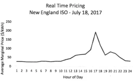
Figure 13: Price of Electricity (July 18, 2017) ... 39

Figure 14: Locations of Homes in Disaggregation Study... 41

Figure 15: Refrigerator's Power Cycle... 42

Figure 16: Summary of Top Deferrable Appliances... 43

Figure 17: Summary of Peak Usage Deferrable Appliances ... 44

Figure 18: ISO-NE Electricity Demand (July 19, 2017) ... 46

Figure 19: Potential for Deferral Based on Metric ... 46

(9)

Tables

Table 1: Pecan Street Results of EEme Disaggregation ... 14

Table 2: Analysis Results Summary ... 32

Table 3: Deferrable Potential of Appliances... 43

Table 4: Peak Deferrable Potential of Appliances... 45

(10)

Chapter 1 - Introduction

1.1 Problem Statement

Most individuals have little knowledge of how energy is distributed throughout their home. In a 2010 survey of over 500 US residential electricity customers, energy use of appliances was underestimated by a factor of 2.8 on average (1). In other words, individuals have a flawed perception on how much energy is being consumed (and wasted) within their home. Non-Intrusive Load Monitoring (NILM) is one of the highest potential methods to alter this

knowledge gap. NILM is a technology that analyzes the steady state and variable power from a single source. This analysis leads to a disaggregation of the power to determine how it is distributed to different appliances throughout the building. In a primary residence context, it could provide information to a resident that they previously did not have access to. The thought is that a residence that has this information would take action to reduce their energy usage. However, introducing NILM into residential homes has a greater importance than just increasing knowledge and reducing the costs of their electricity bill.

In 2015, the electric power industry was the largest single sector contributor to greenhouse gas emissions in the United States (2). Residential electricity customers were the largest portion of this energy usage, and in turn, made up the highest contribution to emissions;

more than commercial or industrial customers (3). While being the highest aggregate source of

emissions, residential electricity consumers are generally unaware of their household energy use until their monthly energy bill arrives. NILM can act as that bridge of engagement between the household electricity use and the user, and motivate to reduce emissions.

With a NILM installed in a residential home, an individual knows the exact costs

associated with running the air conditioner or leaving the lights on downstairs. This information by itself can deter individuals from energy wasting habits. Paired with specific savings

suggestions, comparison and competition with neighbors, and incentives for improving energy efficiency, there is a significant potential for this technology to shift behaviors. Even small behavioral changes at the individual residence level that are widespread can add up to a large impact on society's largest emissions source.

In general, NILM is a technology that has a large potential benefit associated with its widespread usage. These benefits span between multiple stakeholders, including individual

(11)

customers, the electric utility provider, and society at large. At the time of this paper being published, there is no clear adoption strategy associated with the use of this technology. This paper further develops two of the key benefits associated with NILM and provides incentive recommendations associated with each benefit.

The first benefit is studying the effect of a NILM installation in 174 New England homes. Their electricity usage before and after the NILM installation was compared. General energy reduction is important for saving on limited resources. A number of government sponsored incentives are being offered for energy saving appliances installed throughout the home. If NILM devices can prove to reduce energy across a wide sample of customers, a similar incentive program should be considered for these devices.

The second benefit is how NILM can be used as a tool for peak demand reduction. The electric grid capacity is determined by the forecasted maximum electricity demand, better known as peak demand. A sustained reduction in the peak demand can be tied to a reduced cost for utility infrastructure, a reduction in energy purchases from the most expensive generation plants, and savings on the deferral of transmission and distribution (T&D). Aspects of flexibility and power consumed are discussed, with a target appliance range of flexibility and power. An evaluation metric is presented to quantify an appliance deferral potential based on these two aspects of deferral potential.

1.2 NILM Overview

Energy disaggregation is a process by which the overall power usage of a home is broken down into the power consumption of individual appliances. There are a number of different methods to perform energy disaggregation, from simulation models to installing "smart-plugs" at every outlet where an appliance is connected to power.

Non-Intrusive Load Monitoring (NILM) is one such disaggregation method. NILM is widely recognized as one of the most cost-effective methods for gathering disaggregated energy data while maintaining a high level of accuracy. NILM is a method to disaggregate power usage from a single household power-use measurement down to specific appliance usage. NILM makes predictions about which appliances are running by recognizing different patterns and appliance "load signatures". Included within an appliance load signature are the specific power

(12)

NILM devices can identify these key attributes, and filtering these signals from the noise and other devices running at the same time.

1.3 Methods of Disaggregation

Disaggregation via a NILM hardware device will be the primary focus of this paper. However, this is just one of the primary methods for disaggregation of household electricity demand. We will review four different methods of disaggregation of a household power demand: surveys, direct metering, statistical modeling via Advanced Metering Infrastructure (AMI), and hardware installed NILM.

1.3.1 Surveys

One of the lowest cost methods of individual household energy disaggregation is conducting surveys. Surveys are typically conducted on a representative sample of a larger population and results are interpolated to make an estimate about the out-of-sample population. For residential home energy surveys, a survey will make an estimate of the total power consumption based on the appliances that have been listed as part of the home.

Surveys of electricity customers on their consumption can be flawed due to multiple reasons. First, the survey results are only as good as the participants' input. When asking a customer how many refrigerators are running in their house, they may forget about that old fridge in the basement that is rarely opened, but is still consuming electricity. In addition to reporting unintentional inaccuracies, questionnaires themselves can introduce biases that will increase error in the survey reports. Short, clear, and understandable questions will have the most accurate responses, but often the amount of information the surveyor will want to abstract is at odds with this concise recommendation.

As one of the largest surveys of energy disaggregation, the Energy Information

Association's (EIA) Residential Energy Consumption Survey (RECS) provides a depiction of the electricity use of American residences. The survey was first conducted in 1978, initially under the name of the National Interim Energy Consumption Survey (NIECS). The original NIECS has similarities to what you will find published today: approximations for amounts of homes using air conditioning, types of heating fuels used, and conservation efforts performed throughout the year (with many other items covered). The survey was conducted every year until 1984, was

(13)

scaled back to a three-year cycle until 1996, on a four-year cycle until 2009, and is currently conducted every six-years. In 2015, the survey used a combination of in-person interviews and questionnaires to gather data on 5,686 homes from across the country. The data is then put through statistical modeling to determine how the results of the surveyed households apply to other households outside the sample population. The selection of the households involved in the study is highly scrutinized before selection to ensure it is a representative sample of the 118.2 million primary households in the United States (4).

The RECS provides general insights of household energy consumption, long-term trends over time, and are used to shape national energy policy by the EIA and United States Department of Energy. The RECS does not provide any detail information past the state level. In fact, 2009 was the only state-level characterization of data, as 2015 did not receive enough respondents for reporting state-level information. Depending on the objective, this high-level picture of energy consumption can be adequate for modeling purposes. However, when focused on the targeting of specific homes, states, or regions, applying RECS results would provide a large error.

We will use the RECS survey results when discussing general trends in the electric marketplace in Chapter III in order to estimate how many homes have an electric hot water heater and air conditioner in New England.

1.3.2 Direct Metering of Appliances

Another method of disaggregation is to use "smart-plug" sensors, inserted between an appliance and their respective wall outlet. This disaggregation method is often referred to as direct

metering or intrusive load monitoring. This method provides a very accurate power measurement of each appliance; however, it comes at a high cost of purchase and can be timely and disruptive to install throughout the home.

A study performed by the Pecan Street to direct meter 700 volunteer homes in Austin, TX was funded by a $10.4M Department of Energy (DOE) grant. The Pecan Street Dataport is one of the largest publically available datasets for disaggregated home energy usage. The cost of

directly metering the homes was $60-200 per outlet, or approximately $2000 per home (5),

although plug hardware costs have come down since the study was conducted. Current hardware costs for smart plugs vary depending on the functionality offered and user interface. Etekcity@ is

(14)

currently offering their Wi-Fi-enabled, power monitoring smart plugs for $12.50 each (when purchasing four (6)) while WeMo energy monitor smart-plugs are offered at $40 per plug (7).

Direct metering of appliances does have his benefits. It accurately depicts the power usage of an appliance, can give the user wireless control of the appliance and can often be put on an automated schedule. However, at the high cost of installation for direct metering, it is unlikely the wide-spread adoption of this method of disaggregation.

1.3.3 Statistical Modeling via AMI

Another disaggregation method makes predictions of individual home appliance consumption based on reading from advanced meter infrastructure (AMI). AMI captures the total power usage of a home at specific time intervals. This is typically at a 15-minute interval for the most

common type of meter in the market today. This interval power consumption can be paired with certain characteristics of the home (square footage, occupancy, number of stories, efficiency, etc.) along with external characteristics (weather, neighborhood comparison, etc.) in order predict what appliances are running at any given time based on a total power consumption.

One significant benefit of this method of disaggregation is the wide-spread adoption rate of the AMI. In 2016, there were over 62M residential AMI installed around the United States, which accounts for 47% of all residences (8). This effort has been sponsored by utilities across the country to enhance communication with customers and advance the "smart-grid" eventually to a support more awareness of time-of-use.

It has been shown that disaggregation from using AMI power usage data can have significant variability for predicting appliance usage accurately. Pecan Street published two papers (9) (10) for a disaggregation service, EEme. Appliance level usage was predicted based on the total household interval power consumption. The AMI predictions were then compared to Pecan Street's "ground-truth" dataset based on their direct metering.

In the first study, reported by Pecan Street in 2015, EEme was provided 15-min interval household energy usage data (total power usage) for 264 homes over a twelve-month period, along with the corresponding weather data. EEme ran this data through their disaggregation algorithms and predicted which appliances were running at what time. This study was attempting to predict the overall monthly consumption of appliances within the home. The second study was

(15)

number of homes was reduced to 10, and the total historic time used was 77-weeks. This study was attempting to predict the hourly usage of a set of appliances.

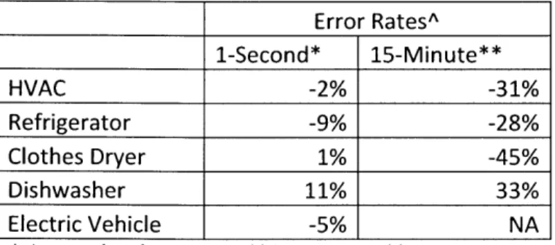
Results for each study are shown in Table 1. It is hard to compare the two results as the 15-minute disaggregation study reports an average monthly error rate, and the 1-second

disaggregation study reports an average hourly error rate. It's possible the 1-second average hourly error rate could aggregate to a larger average monthly error rate, but it is unclear from the results how the two compare. Also, the 1-second data was only based on a limited sample of 10-homes.

What is clear from the study results is that the AMI disaggregation approach used in these studies would not be ideal for real-time disaggregated feedback and energy efficiency validation of appliances. It may be acceptable for some applications i.e. providing feedback to customers on their monthly appliance usage, but it is heavily dependent on the magnitude of error that is acceptable in each application considered.

Error RatesA 1-Second* 15-Minute** HVAC -2% -31% Refrigerator -9% -28% Clothes Dryer 1% -45% Dishwasher 11% 33% Electric Vehicle -5% NA

* Average hourly error rate, **Average monthly error rate,

ANegative _{error rates are underestimates, positive error rates are overestimates}

Table 1: Pecan Street Results of EEme Disaggregation

1.3.4 Hardware Sensors

George W Hart introduced hardware sensor Non-Intrusive Load Monitoring (NILM) in his 1992 paper (11). Since then, NILM has improved in its methods of disaggregation. There are a number of companies that are offering NILM hardware, and although the hardware monitors have gained popularity in the residential market among energy enthusiasts, they are not as nearly wide-spread as AMI. This is likely because of the lack of utility investment in NILM, where AMI received a number of large grants to upgrade the metering system in recent years.

(16)

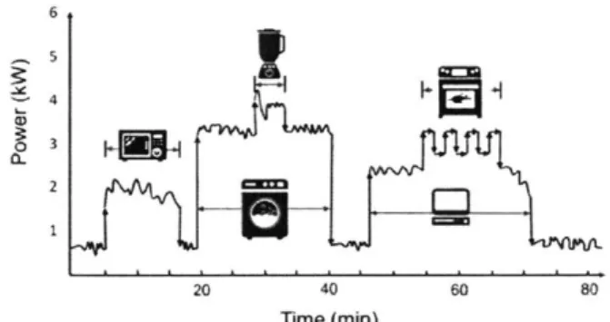
The NILM hardware sensor is installed at a single point within the residence, typically within the circuit breaker panel. The monitor can gather specific data from the break panel connection including real power, reactive power, harmonics, voltage, noise, among other features (12). This aggregate information is matched to a database of known appliance "load-signatures" and from there, a prediction is made about what appliances are running at any given time in the home. As shown in Figure 1, a NILM sensor will break down different appliance usage over time depending on their load signature.

6

4

40 60

Time (min)

Figure 1: Disaggregation via Non-Intrusive Load Monitoring (13)

The primary focus of this paper is around how NILM hardware sensors can benefit the understanding of energy consumption for both the residential customer and the utility.

1.4 NILM Literature review

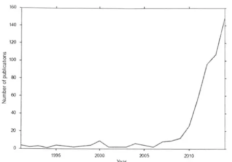
Although the technology for NILM has been around for over 25 years, there has been a

significant increase in interest in the technology in recent years. This is evident by the number of studies that have been published about NILM and the sudden increase in recent years. Reference Figure 2 for a graphic example of this finding.

(17)

160 140 120 100 80 0 .0 E 60 40 20 0 1995 2000 2005 2010 Year

Figure 2: Number ofNILMpublications per year (14)

For a comprehensive survey of different methods of Non-Intrusive Load Monitoring, reference Zoha, et. al., 2012 (15). Within their paper, the authors provide details of the techniques associated with different NILM systems for appliance recognition via energy disaggregation. A general framework of how NILM categorizes appliances based on their load signatures, how these features are extracted and analyzed, and how the state-of-the-art of NILM has moved from supervised learning for pattern recognition to unsupervised learning over the last few years. The paper also provides a clear recommendation for researchers to adopt a common NILM accuracy metric in order to make an adequate comparison between methods. Currently, no such metric exists across studies.

The National Renewable Energy Laboratory (NREL) published a paper and presentation in 2012 describing the potential applications of NILM to different stakeholders including

customers, technology sector, service sector, and utilities (16). Near-term applications of NILM described in the paper include customer and utility gains in efficiency based on appliance level information. Longer-term applications include more automated appliance control of the home based on occupancy as well as predicting faults and failures of appliances.

The remaining portion of literature review will focus on specific use-cases associated with NILM including energy efficiency and targeted demand response.

(18)

1.4.1 NILM for Energy Efficiency

Jack Kelly, 2017 (17), provided a thorough review of twelve energy efficiency studies associated with residential disaggregate electricity usage. Each study was categorized based on having controlled for volunteer bias, the Hawthorne effect, and weather. In addition, just having a control group for comparison was categorized in each study. He claims "to the best of our knowledge, (his thesis) is the first systematic review of domestic, disaggregated electricity

feedback."

Within this paper, Kelly found a wide range of feedback mechanisms to provide the user

information on their home appliances. The average reduction within the twelve studies that were reviewed was 4.5%, which was weighted by the number of households participating in each study. Between the studies, the standard deviation of reduction 10.1%. The greatest effect was

found in an EnergyLife study performed by Gamberini in 2012 which found that disaggregate energy feedback reduced home energy consumption by 38%. The smallest effect was a study by McCalley and Midden in 2002 at 0%. Both the minimum and the maximum usage reduction studies were not for the entire household, but rather a portion of the home (a specific appliance or multiple appliances that were monitored). This is one of the more comprehensive reviews of disaggregate data and its potential for energy savings within the "energy enthusiast" community.

Gupta and Chakravarty, 2014 (18), of Bidgely, studied power usage in California for residential electricity customers who were provided Bidgely's disaggregated services. The results showed for a single month there was a 6% reduction for customers exposed to Bidgely's

disaggregated services compared to customers who were not exposed to the disaggregate information. Although, there is a positive bias associated with customers who opted-in to the

program and chose to have Bidgely services.

Another study performed with Bidgely with Pacific Gas and Electric (PG&E) in California resulted in a 7.7% reduction of customers who were signed up for PG&E's time-of-use (TOU) rates (19). Electricity customers who voluntarily sign up for TOU pricing are assumed to be a positive biased sample of customers. Although these are likely the individuals who have already made energy efficiency progress within their home prior to the study.

Regardless of which bias had more impact on the result, this energy reduction result cannot be directly expected in the general population.

(19)

1.4.2 NILM for Targeted Demand Response

A study completed by Navigant Consulting in partnership with the Advanced Energy Economy (AEE) found that 10% of the country's electricity system is built to meet 1% of the year's hours. This gets to the heart of the need for electricity demand flexibility and the reduction in peak load. If that top 1% of peak load hours is reduced, there are infrastructure cost savings for the utility which translates directly to the rate payer. The same study found for every $1 spent on DR,

benefits were in the range of $3.26 - $4.07 in Massachusetts. These benefits included capacity

market cost avoidance, high energy cost avoidance, transmission and distribution cost avoidance, and greenhouse gas emissions cost avoidance (20).

In a general feedback study, Bidgely worked with Australia's United Energy (UE) to trial

a demand response program (21). The study tracked customer usage and provided real-time feedback during the peak-load events that were called four times over the course of Summer 2015-2016. Gamification via goal setting, immediate real-time feedback, and real-time award confirmation for incentives were part of the Bidgely's "ActionDR" product that was provided to UE's customers. Bidgely reported an "average peak load shift of greater than 30% per user per

event." It is unclear how many homes were involved in this trial-run, however, a greater than 30% reduction in peak usage with no direct appliance recommendations is a noteworthy accomplishment and should be taken into consideration for future work.

The categorization of appliances between deferrable and non-deferrable appliances is

reviewed in this 2017 publication, "Non-intrusive load monitoring through home energy management systems: A comprehensive review" (22). The article details deferrable /

thermostatic appliances (DTA), which are "appliances capable of providing grid services without

jeopardizing the quality and reliability of their primary function according to users' comfort level, and satisfaction" - in other words, appliances that can shift their time of use without the user even realizing. Examples of these appliances within the residence are the electric hot water

heater and air conditioner. These specific deferrable appliances will be the subject of the targeted demand response metric reviewed in Chapter III.

(20)

1.5 Thesis Contributions

The academic achievements of this thesis are as follows:

1. Quantifies the reduction in residential energy usage after a NILM device installation 2. Provide guidelines to improve future energy efficiency studies

3. Identifies a NILM incentive based on similar marketplace efficiency

4. Provides a construct for using appliance-level time-of-use data for demand response evaluations

First, home energy usage before and after installing a NILM device has been studied. Prior to the NILM installation, it was assumed customers only had access to a total electricity consumption via the monthly bill provided from their utility provider. The NILM device

provided both overall power consumption and appliance-level consumption information in real-time via a smart-phone application. The hypothesis is that this additional information was used to take action to reduce overall energy usage. We have tested this hypothesis against actual

customer energy usage data on 174 homes and have confirmed a 2.6 -3.1% reduction after the a

NILM device was installed. We also show how altering the analysis method effects the results. As a second primary contribution, this thesis provides a list of recommendations for performing analysis of energy efficiency studies. There are a number of improvements that could be made within data collection, and study design that are reviewed.

A third contribution of this thesis provides a recommended incentive strategy associated with NILM promoting energy efficiency within the home. A rebate could be provided by federal or state government funds based on the efficiency improvements gained. This type of rebate for NILM devices does not currently exist.

A fourth contribution of this thesis answers the question of how to evaluate the appliance time of use for different applications. This thesis provides a simple deferral metric that can be calculated for each appliance to determine the available shift in demand that could occur. With this metric, each appliance within the home can have its own score of deferral potential. These individual appliances can be aggregated to determine a household deferral score. This household deferral score can be paired with recommendations from the utility for involvement in demand response programs or time-of-use rates. The individual terms of the metric, flexibility and power consumption, can be used for evaluating the shift of appliance usage outside of a peak load timeframe.

(21)

Chapter 2 - Residential Energy Consumption Reduction

2.1 Introduction

The majority of residential electricity customers have a knowledge gap between using their appliances and paying their electricity bill. The bill generally comes on a monthly cycle, and automatic payments online make it easier to ignore the energy bill all together, resulting in less concern for electricity consumed within the home. Unless a bill is significantly higher than expected, the home's residential electricity consumption is an afterthought for most customers.

NILM attempts to change this typical monthly energy feedback in a significant way. With a NILM device installed in the home, immediate feedback associated with electricity usage is possible. The goal behind this study was to determine if there was a reduction associated with that feedback, i.e. are residential customers taking action on the feedback they are receiving?

Using a number of different analysis methods, the monthly energy usage of 174 homes with a NILM device installed was reviewed. Looking at all the different analysis methods, the average household energy reduction was 2.3%. This reduction varied between 1.0 - 3.1% depending on the analysis method, if outliers of the data were removed, type of weather

normalization, and seasonality normalization. Only considering the effects within +/- 2y from

the mean results in a 2.6 - 3.1% reduction on average. Each of these analysis methods are explained in more detail in the Analysis Methods and Results Section 2.4.

2.2 Data for Study

Company X is a distributor of electricity to a large portion of the New England population. The data used for this research was based on 174 Company X electricity customers that had ordered and installed a NILM Home Energy Monitor (HEM). The installation date of the HEM was matched with the home's monthly power consumption data. An automated matching algorithm was used to link the shipping address of the HEM to a billing account, which could output a random house number to the installation date of the HEM, the monthly power bill (in kWh), and the zip code of the home. This automated matching algorithm was used to keep all detailed

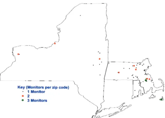
customer information anonymous. Figure 3 shows the distribution of home locations that were a part of the analysis.

(22)

Key (Monitorm per zip code)-''

I Monitor *

40

5

9 Monitors

Figure 3: Locations of Homes in Energy Efficiency Study

To be included in the study, the residence needed at least two months of usage data after the HEM device was installed and 12-months of usage information before the HEM was

installed. Any "net-metering" homes within the data, which is linked to solar-generation, were removed as the information available was only for total billed kWh, rather than the actual energy used within the homes.

In order for account for seasonality pattern recognition within the household usage data, there needed to be a minimum of 24-continuous months of bill usage at the household billing account available. This was a requirement of the software package used to detect seasonality effects (R's seasonal trend decomposition). In other words, the billing account information needed to be continuous for two years. For the analyses that required seasonality decomposition, this eliminated a number of homes from the original 174, down to 146 residences.

(23)

The zip code of the house was incorporated to control for weather in one model. The number of heating degree days (HDD) and cooling degree days (CDD) for each weather station location in the state was averaged to produce a state-wide HDD and CDD.

A heating degree day (HDD) is a form of degree day used to estimate energy

requirements for heating while a cooling degree day (CDD) is for cooling (air conditioning and refrigeration). The daily HDDs and CDDs were calculated by the different between the specific day's average temperature and 65'F. For example, a day with an average temperature of 75'F is categorized as 10 CDD, 0 HDD. A day that has an average temperature of 55'F would be 0 CDD, 10 HDD. Every weather station in New York, Massachusetts, and Rhode Island was incorporated into a state-wide average number of HDDs and CDDs for each month of study.

This method of "average state-weather" was used in a Model 5's analysis to incorporate the effect of weather in combination with the effects of seasonality and installation of the HEM.

2.3 Experimental Setup

In each of the studies detailed in the energy efficiency literature review of Section 1.4.1, recommendations of how to reduce consumption were presented to residential electricity customers. This experiment was performed with a HEM that did not provide specific

recommendations on how customers can reduce their energy usage. Instead, the HEM provided an interface for customers to view their household energy usage in real time, broken down into individual appliance consumption.

The goal of the experiment was to understand the effect of installing this HEM on a home's power consumption. Individual homes power usage before and after HEM installation was compared. The "control group" was the individual households prior to HEM being installed. The "treatment group" was the individual households after HEM was installed and determining the effect.

The Hawthorne Effect is defined as the "alteration of behavior by the subjects of a study due to their awareness of being observed (23)." The Hawthorne Effect was controlled within this research by matching historic usage information for those customers who sought out the

purchase of the specific HEM. The customers continued their normal activities without knowledge of being involved in this study.

(24)

One primary assumption used in calculating the results was that extreme changes of power consumption were not directly caused by the HEM. It was assumed that any large shift in a residential home's energy usage (positive or negative) was due to outside factors that were not taken into account in the model. The analysis results below show all homes in the dataset as well as comparing it to just the homes within +/- 2 standard deviations (+/- 2a) from the mean. This calculated the effects of the HEM with the extreme values of change removed.

2.4 Analysis Methods and Results

There were six different analysis methods used to examine the individual household usage data, each of the methods returned a different result ranging from 2.6% to 3.1% reduction after

removing the extremes (+/- 2a remained). Analyzing the limited dataset with multiple techniques

confirmed that the relative reduction in usage was not due to the type of analysis used. The analysis method without any normalization was excluded from these results for reasons that will be discussed further in detail in the Model 1 section below.

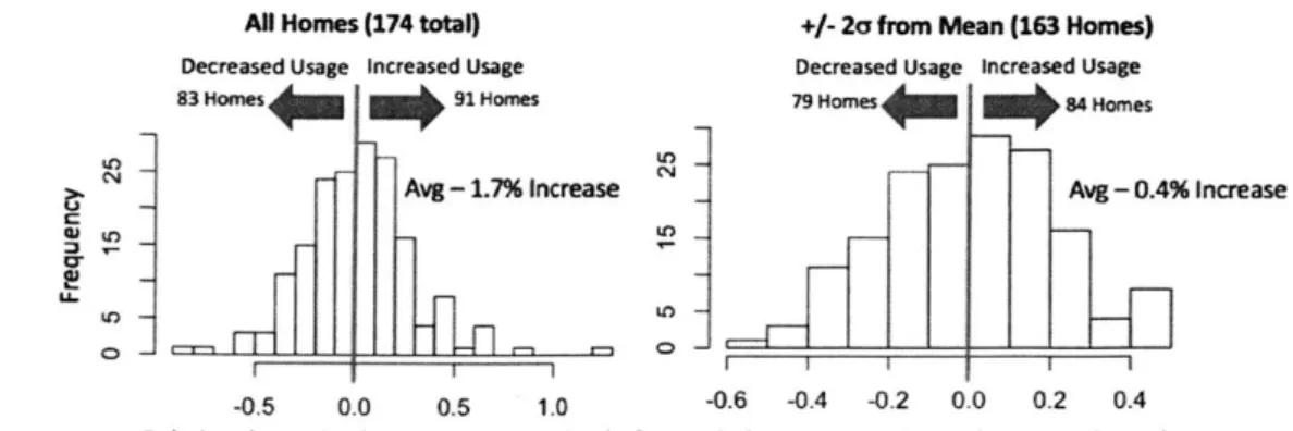
2.4.1 Model 1- Basic Average Comparison

This simple analysis method was used as a reference point, however was not included in the results. It compared the kWh billed before and after the HEM installation for each of the 174 residential homes in the dataset. The results showed that 91 of the homes increased their usage and 83 reduced their usage after the HEM installation. The average effect showed a 1.7% increase in kWh billed after HEM installation. Reference Figure 4 below for the distribution of

results for all homes and the homes within +/- 2a from the mean.

AN Homes (174 total)

Decreased Usage Increased Usage

+/- 2a from Mean (163 Homes) Decreased Usage increased Usage

83 Homes 91 Homes 79 Homes 84 Homes

2

Avg -1.7% Increase Avg -0.4% Ina

I f I I I

-0.5 0.0 0.5 1.0 -0.6 -0.4 -0.2 0.0 0.2 0.4 Relative change in electricity consumption before and after HEM installation (0.0 = No Change)

Figure 4: Model 1 -Basic Analysis Results (No seasonality or normalization)

rease

(25)

This was not included in the summary results stated in the paper's abstract, but it is worth mentioning why it was excluded. Since this model does not take into account any seasonality patterns, it is heavily dependent on when the HEM was installed in the home.

Figure 5 below shows a distribution of when the HEM was installed in each of the homes included in the study. 49% of the HEM devices were installed in the months of November, December, January, or February. When compared to the summer months of May, June, July, and August, which only represented 24% of the total installation months, the winter months have a lower overall power consumption. This the overall trend in the United States, and was seen within this particular dataset. As an example, in the United States, winter months of 2016 (January, February, November, and December) accounted for 15% less energy consumption from the residential sector than did the summer months (May, June, July, August) (24). With the HEM expected to account for a single digit reduction in energy usage for a home, the seasonal usage would dominate the effect of the HEM.

The average time the HEM was installed in the dataset was 7.5 months. Including the summer months and not the winter months in that portion after installation would skew the results. A HEM installed in the winter would include the summer months in the "after HEM" effect. As the analysis only compared the household consumption before and after HEM installation, with the limited number of months included in the after-HEM installation data would skew the results to have an "increased-use" bias.

Distribution of Month Installed

30 25 ' 20 ,.15 10 5

(26)

Based on this information, the month of installation would be a significant factor that could drive the relative change in monthly energy use. For this reason, the results of the analysis Model 1 were not included in the overall results, but for transparency of results and avoidance of errors of any studies pursuing energy efficiency measures in the future, they are worth

discussing.

Comparing direct usage data with imbedded seasonality effects, as Model 1 does, would be a reasonable option to consider with an alternate analysis approach. A control group of "similar" houses that did not have a HEM installed could be used to compare. The similar homes could be based on a monthly power billed (within a certain range) before the HEM installation date. The effect of the HEM installation would be the primary change between the houses, which could be measured for statistical significance. Ideally additional data would be available to compare these "similar-use" homes to one another. This was left for future work as discussed in the Section 2.6 Limitations and Recommendations.

2.4.2 Model 2 - Monthly Normalization

To identify and remove consistent monthly trends in the usage data, a monthly ratio was used to normalize the power data from the 174 homes. This analysis method normalized each month's consumption to the average monthly consumption for that specific household. As an example, a "January Factor" was used for normalizing all consumption data from January. This factor took the overall average consumption for the house and divided it by the average January

consumption. Each month had its own normalizing factor that was multiplied to the actual consumption. When the average consumption for January was lower than the average overall consumption, the month's relative consumption was increased.

When determining the effect that the HEM installation had on the monthly consumption, the normalized average consumption before the installation was compared to the normalized average consumption after installation. This resulted in 99 homes with a reduced usage and 75 homes with an increased usage. The average effect was a 1.0% decrease in the monthly usage after the HEM was installed. Removing the extremes on both ends of the results, and only looking at +/- 2a from the mean resulted in an average decrease in consumption of 2.6%. Figure 6 below shows a distribution of the results of Model 2.

(27)

All Data (174 Homes)

Decreased Usage _{increased Usage}

99 Homes ₇₅_Homes

zizz ₂ z~jIifl

I

Avg - 1.0% Decrease

-I---.

K~

rn

+/- 2cr from Mean (162 Homes)

Decreased Usage Increased Usage 95 Homes 67 Homes

Avg - 2.6% De

...

crease

.0 _5 0.0 00 10 04 4Z 00 02 04

Relative Change in Electricity Consumption Before and After HEM Installation (0.0 = No Change)

Figure 6: Model 2 Results -Monthly Normalization Analysis

2.4.3 Model 3 - Seasonality Removed & Monthly Normalization

This analysis technique used a method to normalize the monthly consumption of each household after the individual household's seasonality trends were removed. Using's R's seasonality

decomposition base-algorithm "decompose", the time series data was identified into three additive portions: a seasonal component, a trend component, and a random component.

Yt = Tt

+

St + Et

Y, is the usage time series, T is the trend, St is the seasonality pattern, and c, is the random remainder

The seasonality component of the usage data was removed, leaving the trend and random components. With the seasonality component removed, the average use was compared before and after the HEM installation. As the decomposition algorithm requires a minimum of two years of data, 28 of the homes in the dataset did not meet this requirement and were removed from the analysis. The remaining 146 homes were analyzed and included in this analysis model.

The results of Model 3 "Seasonality Removed" analysis showed 83 homes reducing their consumption and 63 increasing their consumption. The average effect was a 2.7% decrease, with a standard deviation of 26%. After removing the extremes outside of +/- 2a the average

consumption decrease before and after HEM installation was 2.6%. Reference Figure 7 below for the distribution of results.

C

U, 0)

(28)

Decr U C a) 0' a) LL

All Data (146 Homes) +/- 2a from Mean (136 Homes)

eased Usage Increased Usage Decreased Usage Increased Usage 83Homes - 63 Homes R - 78 Homes 58 Homes

Avg - 2.7% Decrease Avg - 2.6% D

-0.5 MO 0. 1.0 -A -0.2 00 02 0.4

Figure 7: Model 3 Results -Seasonality Removed

ecrease

2.4.4 Model 4 - Seasonality Removed with Linear Regression (Installation only independent variable)

Model 4's analysis procedure started by removing seasonality trends using R's decompose function, similar to Model 3's process. Linear regression was then used to predict the monthly consumption with the installation of the HEM device being the only independent variable in the model.

T= f 1x+E

T -Monthly consumption after seasonality removed, fl, - Individual Home Coefficient for effect of HEM

install, x -Binary variable (0 or 1) representing if the HEM has been installed, E -Random error

With one binary factor that is used in the model to predict overall household power use, it should be no surprise that the linear regression model performed poorly. The model returned an R-Squared of 0.13 indicating the goodness of the fit of the linear regression is extremely low.

This was expected -trying to predict human behavior based on only one independent prediction

variable and a random error term would oversimplify this complexity of how people use power in their homes. Although the model performed poorly in its predicting power, it still provides insight in to the effect of the HEM within the distribution of households.

Aggregating the results of the individual linear regression models showed an average

reduction of 2.7% (i.e. the average

p

within the model was -0.027) with a standard deviation of

(29)

decrease of consumption after the HEM installation was 3.1%. Reference Figure 8 below for the distribution of results.

All Data (146 Homes) +/- 2afrom Mean (138 Homes)

Decreased Usage ncreased Usage Decreased Usage Increased Usage

83Homes M*63 Homes 79 Homes 59 Homes

Avg - 2.7% Decrease _{Avg - 3.1% Decrease}

LI.

-ib 45 0.0 -O -. 2

Figure 8: Model 4 Results - _{Linear Regression (Install Only Variable) with Seasonality Removed}

Looking at the group homes where the installation variable was significant (pStat <0.05) narrows in on the potential for what is likely to be the highest biased set of users - that is the electric customers that were potentially the most engaged with their home energy monitor

feedback. The installation variable was significant for 72 of the 146 homes. Within this subset of 72 homes where the installation of HEM was a significant factor, the average reduction was 4.6%. Removing the extreme values (outside of +/- 2a from the mean), that we can confidently say the power changes were not caused by the HEM, the resulting average consumption

decreased by 5.9%. Reference Figure 9 below for a focused subset of Model 4's results.

All Homes with Significant Installation Factor (63 Homes)

nreased Usa "2 a

+/- 2a from Mean (55 Homes)

Decrnase4 "

5 increased usage sageincreased Usa

39 Homes 24 Homes 35 Homes _{20 Homes}

Avg - 4.6% Decrease Avg - 5.9% Decr

r- --1, -0'5 0.0 04 t.o ' (1 0. 2 ease U C w 0~ a) LL rge

(30)

2.4.5 Model 5 - Seasonality Removed with Linear Regression+ (HDD, CDD, Installation independent variables)

Model 5's analysis removed the seasonality trend using R's decomposition function, similar to Models 3 and 4. Linear regression modeled monthly consumption as the dependent variable with three independent variables - HEM installation (binary), monthly Heating Degree Days (HDDs) and Cooling Degree Days (CDDs) for each home.

T = fl1x + fz H + Ws + E

T -Monthly consumption after seasonality removed, P, - Coefficients of the effect, x -Binary variable (0

or 1) representing if the HEM had been installed, H -HDDs in the state the given month, C - CDDs in

the state the given month, --Random error

Including HDDs and CDDs in the model is a method of controlling for weather. For details associated with HDDs and CDDs, reference Section 2.2.

The goodness of fit of Model 5 was slightly higher than Model 4 (which had the installation being the sole independent variable). Model 5's average R-Squared for the set of households was 0.19, which still shows the model has a poor predicting power. Similar to Model 4's low prediction power, even though this model would not be a strong candidate to predict individual home energy usage accurately, it can still provide insight into the effect of the HEM installation based on the coefficient's trend and significance. However, limitations and

improvements of the model are discussed in the Section 2.6.

The results of the Model 5's analysis of 146 homes showed an average reduction of 2.0% (i.e. the average

Pi

within the model was -0.020) with a standard deviation of 26%. After

removing the extremes and being left with +/- 2cy from the mean, the average decrease of consumption after HEM installation was 2.9%. Reference Figure 10 below for a distribution of Model 5's results.

(31)

Decreased Usage _{Increased Usage}

83Homes _{63 Homes}

S- .Avg - 2.0% Decreas

+/- 2c from Mean (137 Homes)

Decreased Usage Increased Usage

79 Homes ₅₈_Homes

Avg - 2.9% Decrease

.10 00 10 OA 0s 02 0.0 O2 OA

Figure 10: Model 5 Results - Linear Regression' (Installation, HDD, and CDD variables) with

Seasonality Removed

Focusing in on the homes where the installation variable was significant (pStat < 0.05) provided even greater decreases in consumption. The installation variable was significant for 62 of the 146 homes. Within this subset of 62 homes where the installation of HEM was a

significant factor, the average reduction was 4.4%. Removing the extreme values outside the bounds of +/- 2a from the mean, the resulting average consumption decreased by 5.8%. Again, this focused subset of users is likely to be a highly-biased subset of users. Reference Figure 11 below for a distribution of this focused subset of Model 5's results.

All Homes with Significant Installation Factor +/- 2a from Mean (54 Homes)

(62 Home +-2 rmMen(4Hms

Decreased Usage Increased Usage Decreased Usage Increased Usage

38 Homes 24 Homes 34 Homes 20 Homes

Avg - 4.4% Decrease Avg - 5.8% Decrease

Av-.4 eces

U_

L..

...

--o

r

_rr

...

I...

.1--

-1.0 0 0.0 0.5 1.0 .0,4 -02 00 02 04

Figure 11: Model 5 Focused Subset Results - Significant Installation Factor Homes Only

(. C a a U e

(32)

2.4.6 Model 6 - Consistent Time Frame Comparison

Model 6 removed seasonality data using R's seasonal decomposition pattern recognition software. After seasonality was removed, each month's usage was normalized based on its monthly usage factor, similar to the method used in Model 2, except seasonality had been removed prior to normalization.

After normalization, the usage before and after the HEM installation was compared on a consistent time frame - ten months before, and three months after HEM was installed. This was a primary difference between Model 6 and other models.

Three months after installation was chosen as a minimum for this model for multiple reasons. First, it takes time for the HEM monitor to identify devices within the home. It is assumed that the effect of the HEM for reducing energy consumption was based on the

appliance-level feedback. A single month after installation the HEM would not provide the level of details for appliance usage as two or three months after. Therefore, it was assumed that the second and third month would be a better indicator of the longer-term effects of the HEM.

Along those lines, there were multiple homes within the dataset that did not meet the

minimum data on either side of the installation (i.e. a home many have had only 9 months of data before the HEM was installed or the data was only available for two months after installation).

Applying this filter resulted in 130 homes meeting the time frame requirements. Increasing the amount past three months would have reduced the amount of homes we could have included in the analysis further.

The 130 homes that met the three-month minimum time frame for installation showed an overall reduction in energy consumption. The average effect of the HEM installation was a reduction of 3.1%. Focusing in on the +/- 2a from the mean, the average decrease of

consumption after the HEM installation was 2.6%. Figure 12 below provides a distribution of

(33)

Decreased Usage _{Increased Usage} 73 Homes _{57 Homes}

Avg- 3.1% Decrease

+/- 2; from Mean (122 Homes)

Decreased Usage 4 Increased Usage

68 Homes ₅₄_Homes

V - _{Avg - 2.6% Decrease}

F - __ __ _

-0.8- -2 0.0 02 0.4 016 O' -00 2 -03 00 0.1 02 0.3

Figure 12: Model 6 Results - Consistent time frame evaluation with Seasonality Removed and monthly

normalization

2.5 Summary of Results

As described above, there are a number of options for testing the effect of energy reduction. There is no "correct" way to analyze the data, however, providing a spectrum of methods allows a realistic view on the variability an analysis method can have on results.

In all analysis cases with seasonality patterns taken into account, the Home Energy Monitor installation was linked to a decrease in consumption. Averaging the results of across each of these analysis methods gives a 2.3% reduction after HEM installation, which is including all results accept the simple average. Removing the outliers and only looking at results within +/-2a from the mean shows a 2.6% - _{3.1% reduction. Table 2 provides the results from each}

method.

Model Description Results Results (+/- 2a)

1 Simple Average +1.7% +0.4%

2 Monthly Normalization -1.0% -2.6%

3 Seasonality Removed -2.7% -2.6%

Seasonality Removed + Linear Regression

4 (Install Only Variable) -2.7% -3.1%

Seasonality Removed + Linear Regression+

5 (HDD, CDD, Install Variables) -2.0% -2.9%

U

(34)

2.6 Limitations and Recommendations

In this section, we will provide a list of limitations and critiques of this energy efficiency

analysis and recommendations for improvement for similar analysis that may be conducted in the future. There are multiple concerns detailed below that may have had a positive impact on the results, while a number of the concerns may have had a negative impact.

No control group to compare energy savings - As this is a time-based study, the residential

usage before the HEM installation was the "control group" for testing of the hypothesis. The homes in the "test group" were the same as the control, but after the HEM was installed. A potential improvement would be to find similar homes that do not have a NILM device to be compared as a control. A key attribute to show the energy usage difference between the control and the test group would be to match homes that have similar historic usage patterns and

geographic location. This direct comparison of similar homes in a nearby geographic area could remove weather bias and provide stronger evidence of the effect of what is attempting to be tested (in this instance, NILM's effect on energy efficiency). In addition, a properly chosen control group could remove the need to normalize for seasonality and weather since the homes would see the same patterns.

Biased sample - The HEM customers that were a part of this research were likely all "energy-enthusiast" consumers that opted-in to obtaining a NILM device. That is, these customers sought out the purchase of the NILM device, installed the device themselves in their breaker panel (which requires a knowledge of electricity) or potentially paid to have it installed by a

professional electrician. These NILM owners are not the average residential electricity customer. The biased sample could show the associated energy reduction results may be greater than what would occur in the general population of electricity customers.

There is also the likelihood that these energy-conscious customers were making efficient changes to their home prior to the NILM installation. This would be an argument that the

introduction of NILM to less energy-conscious individuals could result in a greater reduction of energy usage. It is uncertain which side of the "opt-in bias" has a greater effect on the results of this study, which is an additional limitation.

(35)

Seasonality Removal Error - A number of analysis methods described above are dependent on R's seasonality decomposition software (Models 3 -6). Recognizing seasonal patterns for a single home's energy usage year-after-year, and removing that pattern, may have a larger effect than the Home Energy Monitor itself. Although a necessary step to attempt to remove seasonal patterns, it would be ideal to ensure each home is modeled next to a control group of similar homes to verify energy reductions. It is also possible to aggregate a number of homes' energy usage in the seasonality decomposition step. This could be completed in a controlled experiment where homes in the same zip code install the HEM on the same date (or close to the same date) and their usage information is summed together. For our analysis, zip codes and the date installed did not match between houses for the aggregation to occur.

Sustainability of Savings - The average timeframe the test group had the HEM installed was seven months at the time the study was conducted. A future study could confirm the sustained effect years into the future with continued engagement of the customer. This would confirm customers taking action to reduce their electricity consumption have not fallen back into the prior usage trends.

No direct energy efficiency feedback was provided to the customers - The NILM device

installed came with an application showing the usage in kilowatt hours (kWh) and also the cost associated with that usage for each appliance. There was no additional feedback to alter

customers' behavior to reduce energy usage. It has been shown that adding gamification and specific actionable feedback can lead to a greater reduction in consumption.

Passive NILM device - There was no control over individual appliances through the NILM feedback application. In order to take action on the disaggregate information they received, customers would need to take an additional step to reduce their usage by changing a setting on an appliance or adjusting their behavior in some manner. It is assumed that the magnitude of energy reduction will increase as more control is integrated into the HEM feedback mechanism.

For example, the application would recognize an outlier day that the air conditioner was running nearly all day (on an extremely hot day). The app would then send a notification stating