Atmospheric oxygen of the Paleozoic

HAL Id: insu-03191494

https://hal-insu.archives-ouvertes.fr/insu-03191494

Submitted on 7 Apr 2021

HAL is a multi-disciplinary open access

archive for the deposit and dissemination of

sci-entific research documents, whether they are

pub-lished or not. The documents may come from

teaching and research institutions in France or

abroad, or from public or private research centers.

L’archive ouverte pluridisciplinaire HAL, est

destinée au dépôt et à la diffusion de documents

scientifiques de niveau recherche, publiés ou non,

émanant des établissements d’enseignement et de

recherche français ou étrangers, des laboratoires

publics ou privés.

Distributed under a Creative Commons Attribution - NoDerivatives| 4.0 International

Atmospheric oxygen of the Paleozoic

Uwe Brand, Alyssa M. Davis, Kristen K. Shaver, Nigel J.F. Blamey, Matt

Heizler, Christophe Lécuyer

To cite this version:

Uwe Brand, Alyssa M. Davis, Kristen K. Shaver, Nigel J.F. Blamey, Matt Heizler, et al..

At-mospheric oxygen of the Paleozoic.

Earth-Science Reviews, Elsevier, 2021, 216, pp.103560.

Earth-Science Reviews 216 (2021) 103560

Available online 27 February 2021

0012-8252/© 2021 The Author(s). Published by Elsevier B.V. This is an open access article under the CC BY-NC-ND license (http://creativecommons.org/licenses/by-nc-nd/4.0/).

Review Article

Atmospheric oxygen of the Paleozoic

Uwe Brand

_{, Alyssa M. Davis}

_{, Kristen K. Shaver}

_{, Nigel J.F. Blamey}

_{, Matt Heizler}

_,

Christophe L´ecuyer

a_{Department of Earth Sciences, Brock University, 1812 Sir Isaac Brock Way, St. Catharines, Ontario L2S 3A1, Canada} b_{Department of Earth Sciences, University of Western Ontario, 1151 Richmond Street, London, Ontario N6A 5B7, Canada}

c_{Department of Earth and Environmental Science, New Mexico Institute of Mining and Technology, 801 Leroy Place, Socorro, NM 87801, USA}

d_{Laboratoire de G´eologie de Lyon "Terre, Plan`etes Environnement", CNRS UMR 5276, Universit´e Claude Bernard Lyon 1, Ecole Normale Sup´erieure de Lyon, Campus de} la Doua, Villeurbanne F-69622, France

A R T I C L E I N F O Keywords: Paleozoic Halite Fluid inclusions Mass spectrometry pO2 measurements

Direct and indirect proxies

Relatively constant atmospheric oxygen

A B S T R A C T

The evolution of Earth’s atmosphere is of extreme importance to the lithosphere, hydrosphere and biosphere. This is particularly true for the role the biosphere played in the inceptual formation of atmospheric oxygen, and subsequently in its potential role in the evolution of higher life forms. Quantifying the change in atmospheric oxygen with geologic time is extremely challenging, with the redox sensitive isotope and element models subject to contradictory outcomes. Here, we present a new approach in determining past atmospheres, by a) directly measuring (DM) the amount of atmospheric oxygen trapped in fluid-gas inclusions of primary and unaltered halite, and by b) using a back-calculation method (BCM) applied to trapped halite fluid inclusion gas contents subjected to post-depositional biogeochemical reactions to calculate the amount of atmospheric oxygen.

On average (±standard error), atmospheric oxygen content during the latest Ediacaran was 17.4 ± 2.1% compiled from DM of 17.4 ± 1.3% and from BCM of 17.3 ± 2.9%. For the earliest Cambrian average oxygen was 19.3 ± 1.4% compiled from DM of 18.8 ± 1.5% and from BCM of 19.8 ± 1.3%. The oxygen content during the mid and late Ordovician was relatively invariant with 15.6 ± 1.8% [15.4 ± 1.4% (DM), 15.8 ± 2.2% (BCM)], and 16.2 ± 1.2% [15.7 ± 1.7% (DM), 16.6 ± 0.7% (BCM)], respectively. The relatively stable atmospheric oxygen levels continued into the Silurian of 15.9 ± 1.1% (12.9 ± 0.4 to 16.5%, DM; 14.3 ± 1.7 to 19.8 ± 2.1% BCM) except for a peak to about present levels during the late Silurian of 23.2 ± 1.9% (21.6% DM, 24.7 ± 3.7% BCM). Early Carboniferous atmospheric oxygen returned to relatively lower and invariant levels at about 15.3 ± 0.7 to 15.7 ± 1.0% (15.0%, 15.5 ± 0.1% DM, 9.4 ± 3.9 to 15.8 ± 1.9% BCM). Similarly, the average atmospheric oxygen content in fluid inclusion of halites from the late Permian was similar with 15.7 ± 1.3% with 16.9% (DM) to 14.5 ± 2.6% (BCM). Indeed, our study suggests that atmospheric oxygen was relatively constant for most of the Paleozoic at about 16.5% (±0.6 SE, ±2.2 SD). This puts our proxy result at odds with the values and trends suggested by the COPSE, GEOCARBSULF AND GEOCARBSULFOR models for the early Paleozoic atmospheric oxygen, and continues the discord with the GEOCARBSULF and GEOCARBULFOR models during the late Paleozoic.

1. Introduction

Researchers have debated the origin and evolution of atmospheric oxygen for some time, with quite contradictory opinions (e.g., Rubey, 1951; Holland, 1962; Berkner and Marshall, 1965; Rutten, 1970; Garrels et al., 1973; Schidlowski et al., 1975, 1977; Walker, 1977; Towe, 1978;

Budyko and Ronov, 1979). Eventually, Berner (1987) formulated a model with an oxygen trend for the Earth’s atmosphere (Fig. 1). The

oxygen content of the atmosphere is reconstructed using either nutrient/ weathering models, and/or mass balance models using either proxy data of carbon and/or sulfur isotopes, or proxy data of redox sensitive ele-ments/minerals. The last few decades have seen a dramatic increase in the number of variants in the nutrient/weathering model, the isotope mass balance model, proxy inversion model, as well as in redox-sensitive element models trying to predict atmospheric conditions, especially oxygen contents of the geologic past (e.g., Mills et al., 2016).

* Corresponding author.

E-mail address: ubrand@brocku.ca (U. Brand).

Contents lists available at ScienceDirect

Earth-Science Reviews

journal homepage: www.elsevier.com/locate/earscirev

https://doi.org/10.1016/j.earscirev.2021.103560

Unfortunately, despite this great substitute number for volume increase of studies about atmospheric oxygen contents most model predictions remain contradictory, and a consensus on a unified atmosphere model for Earth’s history, including the Paleozoic, remains elusive (e.g.,

Lasaga, 1989; Butterfield, 2011; Stolper et al., 2016; Large et al., 2019;

Steadman et al., 2020; Algeo and Liu, 2020; Bennett and Canfield, 2020;

Liu et al., 2021).

In subsequent years, Berner and his colleagues revised, updated, and refined the concept of the carbon and sulfur cycles transitioning from various versions of the GEOCARB to the GEOCARBSULF models (Berner, 1991, 1994, 2006a, 2006b, 2009; Berner and Canfield, 1989; Berner and Kothavala, 2001; Berner et al., 1983, 2000, 2007; Royer et al., 2014). The sum total of reconstructions based on his group’s various models are presented in Fig. 1 with atmospheric oxygen during the Paleozoic ranging from a low of about 10% pO2 during the mid Ordovician to a

high of 35% during the late Carboniferous – early-mid Permian, while entertaining age bins of about 10 million years. Also, the adoption of carbon isotope compositions of deep-time biogenic carbonates without due consideration for a) geographic-specific, b) species-specific varia-tions and c) whether individual populavaria-tions represent truly global conditions makes for an immensely oversimplified δ13_{C signal (Brand} et al., 2015; Ullmann et al., 2017). The variations can be as large as 5.3‰, and without a sufficiently large database for each time period may give a false impression of large excursions (e.g., ~4.9‰ Devonian,

van Geldern et al., 2006; ~4.5‰ Carboniferous-Permian, Grossman et al., 2008) as documented by modern brachiopods from low and mid latitude regions with a total range of 5.3‰ δ13_{C (Brand et al., 2015).}

Furthermore, the atmospheric oxygen reconstructions are highly dependent on original carbon isotope compositions (e.g., Saltzman, 2005; van Geldern et al., 2006; Grossman et al., 2008), which of course are difficult to assure for both biogenic and abiogenic carbonates (cf.

Brand and Veizer, 1981; Brand, 2004; Zaky et al., 2019). However, at-mospheric modelling based on carbon isotope compositions of well- preserved carbonates from low and mid latitudes may minimize the error, in part, documented by the continually shifting’ atmospheric oxygen trends in Fig. 1.

Nevertheless, the work by Berner’s research group inspired others to use redox sensitive elements, sedimentary charcoal (inertinite) and other proxies to model or constrain the oxygen content or its limits

during the Phanerozoic. Fig. 2 presents an overview, far from complete, of modelled atmospheric oxygen contents for the Paleozoic (e.g., Berg-man et al., 2004 [COPSE model]; Algeo and Ingall, 2007; Glasspool and Scott, 2010 [Wildfire Window model]; Arvidson et al., 2013 [MAGic model]; Krause et al., 2018 [GEOCARBSULFOR model]; Lenton et al., 2018 [COPSE reloaded model]; Schachat et al., 2018; Zhang et al., 2018;

Liu et al., 2021 [evaluation of GEOCARBSULF and COPSE models];

Large et al., 2019 [Pyrite-RSE model]. The model reconstructions are quite variable and different (Fig. 2), and clearly speak to the lack of consensus (e.g., Stolper et al., 2016) on atmospheric pO2 with geologic

time including the Paleozoic (e.g., Mills et al., 2016; Algeo and Liu, 2020). But more importantly it speaks to the fact that models may inherently be complex manifestations, but are still a simplification of real-world conditions. This disparity is complicated by the lack of any direct calibration of ancient redox environments with modern counter-parts (Bennett and Canfield, 2020) and thus atmospheric oxygenation levels, and whether redox sensitive elements (RSEs) and redox sensitive isotopes (RSIs) used in the box models from specific environments and localities relate to and reflect global oceanic/atmospheric conditions.

In contrast, Large et al. (2019) used a different approach based on the redox sensitive element geochemistry in sedimentary pyrite rather than those in bulk rock shale/limestone (cf. Krause et al., 2018). Their model depicts a cyclicity in atmospheric oxygen with regular oxygen lows corresponding to nutrient deficiency and major mass extinction events. Also, Lasaga (1989) proposed a new approach to modelling atmospheric oxygen contents by considering different inputs and statistical methods of model outputs. However, none of these models whether based on nutrients/weathering, carbon and sulfur isotopes or redox sensitive el-ements have generated a Paleozoic atmospheric history that is consistent with physical and biological constraints (e.g., Berner et al., 2000; Dahl et al., 2010) such as animal and/or plant evolution (e.g., Butterfield,

Berner 2001 Berner 2006a Berner 2009

Tr

P

C

D

S

O

C

E

Fig. 1. Summary contents and trends of atmospheric oxygen for the Paleozoic

based on various models of the Berner research group such as GEOCARB (Berner, 1987, 1991), GEOCARB II (Berner, 1994), GEOCARB III (Berner and Kothavala, 2001), and GEOCARBSULF (Berner, 2006a, 2009). For discussion of the various models see the aforementioned research papers.

Age (Ma)

C

D

S

O

E

P

Tr

p

O

(%)

C

Royer et al. ( 2014) Lenton et al. (2018) Schachat et al. (2018) Arvidson et al. (2013) Zhang et al.(b) (2018) Large et al. (2019) Glasspool & Scott (2010)

Zhang et al.(a) (2018) Krause et al. (2018)

Fig. 2. Summary contents and trends of modelled atmospheric oxygen for the

Paleozoic based on numerous authors and models such as MAGic (Arvidson et al., 2013), COPSE (Bergman et al., 2004), and GEOCARBSULFOR (Krause et al., 2018); for Berner’s research group’s results see Fig. 1). Included are several variations on the four major models. Not all authors and their publi-cations have been included for clarity and due to space limitations (e.g., Freyer and Wagener, 1970; Lasaga, 1989; Beerling et al., 2002; Glasspool and Edwards, 2004; Holland, 2006; Lawrence et al., 2006; Scott and Glasspool, 2006; Dahl et al., 2010; Glasspool and Scott, 2010; Stuart et al., 2016; Cole et al., 2017; Edwards et al., 2017; Wallace et al., 2017; Mills et al., 2019; Liu et al., 2020). For discussion, ranges and uncertainties of the individual average values/trends see the listed publications and references therein.

2011; Lenton et al., 2018; Graham et al., 2016). Probably, the best constraint on the lower and upper limits of atmospheric oxygen content comes from the so-called ‘wildfire window’ which ranges from 15% for the ‘lower limit’ to 35% for the ‘upper limit’ of pO2 for wildfires based on

fire residues (inertinite) found in all geological periods since the mid- late Silurian (Scott, 2000; Scott and Glasspool, 2006; Glasspool and Scott, 2010; Liu et al., 2020). The lower limit is hampered mostly by a lack of evidence or in the difficulty of preserving suitable wildfire res-idue in the rock record.

Although the preponderance of models from COPSE (Bergman et al., 2004) to GEOCARB (Berner 1990) to GEOCARBSULF (Berner, 2006a) to GEOCARBSULFOR (Krause et al., 2018) has increased the believability of generated atmospheric oxygen models and trends, but, according to

Holland (2006, p. 911) “…direct confirmation of the calculated O₂ levels is still needed.” The inquiry into the evolution of atmospheric oxygen has endured, because according to Holland et al. (1989, p. 362) “…we have no samples of unaltered, geologically old air.”. His opinion remained valid up until 2016, when this concept was dramatically changed by the study of Blamey et al. (2016) who presented evidence of ‘ancient air’ trapped in bubbles within fluid inclusions of primary halite from the Neoproterozoic of Australia. Blamey et al. (2016) had revived and improved on a method presented by Freyer and Wagener (1970) of measuring atmospheric oxygen trapped in fluid/gas inclusions of pri-mary halite from the Permian Zechstein of Germany. Blamey et al. (2016) demonstrated that diagenetically screened halite, from the 815 million year-old Browne Formation of Australia, with its primary petrographic features and geochemical signatures documented an at-mospheric oxygen content of 10.9% for the mid Tonian (cf. Blamey and Brand, 2019). Their study represents the first direct measurement (DM) of atmospheric oxygen in Neoproterozoic air, and it demonstrates the great potential of halite fluid inclusions as archives and direct proxies of original ancient and modern atmospheric air along with its oxygen content (cf. Freyer and Wagener, 1970). This potential of halite to carry original, ambient atmospheric oxygen must be clearly documented by the rigorous screening of the rock salt for primary features among them chevrons while avoiding post-depositional features such as deforma-tional grain boundary migration and the accompanying generation of secondary fluid-gas inclusions cross-contaminated by post-depositional air of unknown affinity or replacement by clear and fluid-inclusion free halite (e.g., Goldstein, 2001; Blamey and Brand, 2019; Peach et al., 2001; Roedder, 1984).

Bennett and Canfield (2020, p. 1) sum up best the inherent weak-nesses in the RSE and RSI-based models “Redox-sensitive trace metals have been used extensively as geochemical proxies to infer the redox- status of marine sediments at the time of deposition, and by extension, the concentration of oxygen in the overlying water atmosphere.” Going from local/regional depositional systems to global ocean and atmo-sphere systems is huge and complicated and as a minimum requires calibration and confirmation of the primary nature of the proxies after diagenesis and often mild metamorphism (cf. Bennett and Canfield, 2020). Thus, box models by estimating sources and sinks may produce inconsistent oxygen predictions (Fig. 2; e.g., Krause et al., 2018; Liu et al., 2021) of rather complex real world conditions.

Our first objective is to determine past atmospheric oxygen levels by measuring gas trapped within fluid inclusions of deep-time primary halite and evaluate its merit compared to traditional RSE and RSI model results. Thus, we will examine a number of Paleozoic and some Edia-caran halites for primary features (cf. Blamey and Brand, 2019) that may guide us to suitable gas inclusions for direct atmospheric gas measure-ments (DM). Another objective is to characterize the observed trend of combined methane (CH4) and carbon dioxide (CO2) gases

bio-geochemically formed and trapped in fluid/gas inclusions of modern halite to its ancient counterparts and subsequently determine the oxygen content of the original ambient atmosphere using a back calculation measurement (BCM) method. Finally, we will compare our direct mea-surement (direct proxy) and back-calculated meamea-surement (indirect

proxy) of atmospheric oxygen contents to the major model-based at-mospheric oxygen reconstructions of the Paleozoic. However, before this is done, all atmospheric oxygen measurements whether ‘direct’ or ‘indirect’ (through back-calculation) will be calibrated and tested against modern marine and non-marine halites from a number of global localities, as well as against trapped laboratory air.

2. Sample Material

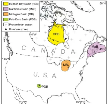
Halite material for this study came from cores of the late Ordovician of the Hudson Bay Basin of northern Ontario, Canada (Zhang, 2011;

Davies, 2018), the late Silurian of the Michigan Basin of southern Ontario (Davies, 2018), the Carboniferous of the Maritimes Basin of Nova Scotia and New Brunswick, Canada (Shaver, 2018), the early Silurian Mallowa salt of the Carribuddy Group of the Canning Basin, Australia (Cathro et al., 1992), and the Permian Palo Duro Basin of Texas, United States of America (Knauth and Beeunas, 1986; Fig. 3). The results are compiled in Table 1 and listed in Appendix 1. These results are supplemented by previously published data from the Ediacaran Hongchunping (China) and Salt Range (Pakistan) formations (Meng et al., 2011; Blamey et al., 2016), the Cambrian Ara Group (South Oman;

Schoenherr et al., 2007; Blamey et al., 2016), the mid Ordovician Majiagou Formation (China; Ran et al., 2012; Blamey et al., 2016), and the end Permian Zechstein Formation of Germany; representing the classical gas results of Freyer and Wagener, 1970. The supplemental data are summarized in Table 1 and included in Appendix 2.

3. Methods

All halite material was cleaned of organics and non-halite contami-nants prior to gas and geochemical analyses. Then, the specimens were visually inspected for cloudiness or clear features to help identify suit-able layers with fluid inclusions. Once a suitsuit-able area/layer was iden-tified and passed the screening protocol (discussed in next section), it

60°N 110°W 80°W 60°N 80°W

U. S. A.

C A N A D A

Precambrian craton Borehole (core) Maritimes Basin (MaB) Michigan Basin (MB) Palo Duro Basin (PDB)

45°N

Fig. 3. Paleozoic basins of North America. Halite was retrieved from cores

spanning the upper Ordovician (Red Head Rapids Formation, Hudson Bay Basin, Canada; Davies, 2018), the upper Silurian (Salina A2 and B units, Michigan Basin, Canada & U.S.A.; Davies, 2018), the Visean (Stewackie and upper McDonald Formations, Maritimes Basin, Canada; Shaver, 2018), and the upper Permian (Salado Formation, Palo Duro Basin, U.S.A.; Knauth and Beeu-nas, 1986). (For interpretation of the references to colour in this figure legend, the reader is referred to the web version of this article.)

was sectioned or cleaved for petrographic thick sections and comple-mentary material was set aside for gas and geochemical analyses. For the geochemical analysis, sample material was dissolved in deionized water and analysed at a commercial lab (Actlab, Ontario) using an ICP-MS (Table 1). Reproducibility of Br analyses was better than 1.5%, with a method blank detection limit of 0.1 ppm.

Halite material for gas analysis was cleaned with isopropanol alcohol and allowed to air dry. Clean chips were then placed into the crushing apparatus and pumped overnight to low vacuum to remove all adsorbed and interstitial gas. Similarly the mass spectrometer was pumped over-night to low vacuum of about 10−8 _{Torr, principle remaining gas being}

water vapor. The following day, samples were incrementally crushed and released gas was measured for H2, He, CH4, H2O, N2, O2, Ar and CO2

during continuous flow ‘dynamic mode’ with a Pfeiffer Prisma quadru-pole mass-spectrometer. Results were garnered from the mass spec-trometer chamber before insertion of gas, during streaming of gas from halite, and afterwards upon completion of streaming to correct for background conditions. The mass spectrometer cycled sequentially through the gases of interest, and each gas content was characterized by 200–400 cycles of molecular gas acquisitions. The crushing chamber with sample and the mass spectrometer were pumped down to low vacuum between each crush and next gas analysis. This whole process may be repeated up to twelve times depending on the size of the sample and the presence of resolvable fluid inclusion gases. All gas results are reported on a water-free and blank-adjusted basis (Appendices 1, 2). The

Bonaire halite sample with its zero air content was utilized as an analytical blank to monitor the leakage of air into halite. The mass spectrometer was calibrated with Scott Minimix calibration gas mixtures and with three in-house natural fluid-inclusion standards (Blamey, 2012; Blamey et al., 2015). The mass spectrometer’s detection limit for atmospheric gas is ~1 f (10−15_{) mols (Blamey et al., 2015), and is an}

essential ingredient in ‘plucking’ gas results from the ‘tiny’ gas bubbles within the small fluid inclusions of 10−10 _{to 10}−13 _{mols (Appendix 1, 2).}

Microthermometry work was done at the Western University lab on cleaved halite wafers. Homogenization temperatures were determined with a Linkham stage microscope system, and accuracy was 0.1 ◦_{C for}

melting of ice to water at 0.0 ◦C. Reported temperatures are within the

range of ancient primary depositional halite (Table 1).

For statistical analyses and plotting of gas contents we used the free- ware PAST3 (v 3.14, Hammer et al., 2001). Evaluation of DM and BCM gas results was done with parametric (t-test) and non-parametric (Mann- Whitney U) tests (Table 2).

4. Diagenetic Screening

The integrity of the halite and its gas-hosted fluid-inclusions is of great importance in obtaining original and ambient atmospheric gas concentrations. To address this question, Blamey and Brand (2019)

proposed a screening protocol that identifies material with the greatest potential of preserving primary inclusions and original gas contents. It is Table 1

Oxygen gas contents (DM: direct measurement, source as marked; BCM: back calculated measurement, this study) of fluid inclusions from various late Ediacaran and Paleozoic halite units, and of modern halite and capillary tubes. Other information (age, Br content, homogenization temperatures (Th), and gas results) from various sources and for geological background.

Period Formation Age DM BCM Other

information Source/Geological Background Ma mol % mol %

Modern halite 0 20.29 ± 2.12 21.41 ± 0.73 Blamey et al. (2016; DM) Modern halite -

Bahamas 0 19.91 ± 0.89 21.63 ± 0.79 Blamey et al. (2016; DM) Capillary Tubes 0 20.98 ± 0.35 Blamey et al. (2016)

Ediacaran Hongchunping 545 17.2 ± 0.4 (3) 17.7 ± 4.9 (6) 16.4–39.4a _{Meng et al. (2011); Blamey et al. (2016; DM)}

Salt Range 545 17.6 ± 2.2 (7) 16.9 ± 0.8

(24) 79 Br ppm Kovalevych et al. (2006); Blamey et al. (2016; DM) Salt Rangeb _{545 26.4 ± 1.3 (5) This study}

Cambrian Ara Group 542 18.8 ± 1.5 (2) 19.8 ± 1.3

(25) 145 Br ppm Amthor et al. (2003)(2016; DM) ; Schoenherr et al. (2007); Blamey et al. Ordovician Majiagou 465 15.4 ± 1.4 (2) 15.8 ± 2.2 (4) 163 Br ppm Ran et al., (2012); Hu et al. (2014)

14.7–36.9a _{Blamey et al., (2016; DM)}

Red Head Rapids 445 15.7 ± 1.7

(12) 16.6 ± 0.7 (32) 358 Br ppm This study; Zhang (2011) Red Head Rapidsc _{445 7.4 ± 1.1 (8) This study}

Red Head

Rapidsb 445 22.2 ± 5.6 ₍₁₀₎ This study

Silurian Mallowa Salt 442 12.9 ± 0.4 (2) 14.3 ± 1.7 (8) 157 Br ppm This study; Williams (1991); Cathro et al. (1992) Salina A2 425 21.6 24.7 ± 3.7

(14) 13.3–35.2

a _{This study; Brennan and Lowenstein (2002)}

Salina A2b _{425 20.4 ± 6.6 (6) This study}

Salina B 422 16.5 19.8 ± 2.1

(35) 86 Br ppm This Study; O’Shea et al. (1988) Carboniferous Cassidy Lake 337 15.0 15.5 ± 1.3 (6) This study; Hovorka et al. (1993)

Stewackie 336 15.2 9.4 ± 3.9 (8) 22.7–31.2a _{This study; Holt et al. (2014)}

U McDonald 335 15.5 ± 0.1 (2) 15.8 ± 1.9

(16) 16.1–18.9

a _{This study; Holt et al. (2014)}

149 Br ppm

U McDonaldb _{335 21.5 ± 3.2 (7) This study}

Permian Salado (1) 260 24.2 ± 3.2

(8)b This study; Hovorka et al. (1993)

Salado (2) 259 16.9 14.5 ± 2.6

(10) 111 Br ppm This study; Knauth and Beeunas (1986) Zechstein 253 14.7 (20) 2.4 to 43.3c _{Freyer and Wagener (1970); Zhang et al. (2013)}

Note: DM: mean ± standard error; BCM: mean intercept value at 0% OMG ± standard error. All results are reported in Appendices 1 and 2; modern halite results are in

Blamey et al., 2016 and Blamey and Brand, 2019.

a_{Microthermometry- homogenization temperatures in} ◦_C. b _{Result of ‘leaked’ fluid inclusion gas.}

a multi-step screening process consisting of: 1) visual inspection of halite for primary depositional fabrics and opacity (Fig. 4), 2) petrographic inspection of primary fluid-inclusion fabrics such as chevron fluid in-clusion trails, alternating light and dark chevron bands, cornets, and hoppers (Fig. 5A, B, D, F; e.g., Casas and Lowenstein, 1989; Benison and Goldstein, 2000; Schreiber and El Tabakh, 2000; Goldstein, 2001) and secondary (diagenetic) features such as dissolution and recrystallization (Fig. 5A) and microfractures with associated bubbles (Fig. 6; e.g.,

Lowenstein and Hardie, 1985; Schl´eder and Urai, 2005; Schoenherr et al., 2007), 3) homogenization temperatures of trapped fluids within inclusions consistent with depositional/environmental conditions (Table 1; e.g., Benison and Goldstein, 2000), 4) trace chemistry such as Br contents consistent with primary halite formed from evaporating seawater (>79 ppm, McCaffrey et al., 1987; Table 1), 5) sulfur and/or strontium isotopes to differentiate between marine and non-marine halite and potentially diagenetic types (e.g., Blamey et al., 2016), 6) argon isotope geochemistry for tracking diffusion of gas between in-clusions and ambient reservoirs (Stuart et al., 2016; Blamey and Brand, 2019), and 7) a combination of baseline methane, carbon dioxide and argon contents back-calibrated/calculated to atmospheric gas trapped in modern counterparts and capillary tubes (Blamey and Brand, 2019). New to this study will be the comparison of gas results based on direct measurements (DM, direct proxy) and those obtained by the proposed back calculation measurements (BCM, indirect proxy).

4.1. Diffusion

Addressing a potential concern with diffusion, Zimmermann and Moretto (1996) experimented with both cloudy halite full of chevron and hopper fabrics and clear halite of primary syntaxial and early diagenetic cementation and phenoblastic origins (Schreiber and El Tabakh, 2000). They pumped their samples overnight to remove adsorbed gases, and subsequently heated them in 20 ◦_{C increments to}

determine their gas diffusion response to heating. They noted no release of H2 at heating temperatures below 200 ◦C, with similar observations

for CO2 with log D/a2 of less than 10–19.00 and 10–17.00, respectively

(Suppl. Fig. S1). An important observation is that this temperature is

well above the burial geothermal gradient temperature of most of our studied halite core material. Even at higher temperatures, diffusion of H2 and CO2 is still insignificant from both cloudy as well as clear halite

(Suppl. Fig. S1). Since most salt tectonic processes occur at depths of less than 5 km, lithostatic pressure of less than 120 MPa, and burial tem-peratures of less than 200 ◦_{C (Peach et al., 2001), diffusion under regular}

burial depths should not be a concern as confirmed by log D/a2 _{values of}

less than 10–21.00 _{for CO2 and less than 10}–24.00 _{for H2 (Suppl. Fig. S1).}

Thus, the retention of primary gas contents within bubbles trapped within halite fluid inclusions should be the norm since the sampling depth of most core material rarely exceeds the limits mentioned above. Although, primary chevrons with fluid inclusions may be preserved in halite buried as deep as 5000 m with its original fluid chemistry and gas phase (Bukowski et al., 2020, Fig. 6a–c). This speaks highly to the robustness of halite resisting the vicissitudes of diagenetic alteration and recrystallization even in tectonic settings. Contamination of gas contents is still possible due to syn-depositional recrystallization and/or later disturbance/deformation, and the outcomes of these impacts need to be clearly identified prior to gas analysis. Thus, careful screening of halite material is imperative to the successful acquisition of ‘original’ atmo-spheric oxygen contents and compositions.

4.2. Microstructures & Leakage

The contribution of depositional gases and liquids from halite to atmospheric reconstructions may be complicated by deformation under differential stress that involve dislocation and fluid-assisted dynamic recrystallization and pressure solution processes (Urai et al., 1987;

Peach et al., 2001). Depositional features such as chevrons are easily destroyed by recrystallization and pressure solution processes, and their partial obliteration provides clear evidence of them (e.g., Fig. 5A). Although, halite under many conditions may react like a ductile material to disturbances, under some specific conditions it may fracture and/or microcrack (e.g., Schoenherr et al., 2007) and create intercrystalline and intracrystalline microstructures while generating secondary fluid and/ or gas inclusions (e.g., Popp and Kern, 2001; Schl´eder and Urai, 2005). Halite as a seal to hydrocarbon accumulation and gas evasion is based on three key material properties, such as: 1) hydrofracturing under high fluid pressure (Hildenbrand and Urai, 2003), 2) ductile deformation of salt (Popp and Kern, 2001), and 3) its low permeability (~10−21 _m2_; Peach and Speirs, 1996) even with burial to several 100’s of meters (Casas and Lowenstein, 1989). The small amount of water trapped in halite has an important impact on its rheological properties by facili-tating fluid-assisted grain-boundary migration and pressure solution (e. g., Schl´eder and Urai, 2005), with microcracking and grain boundary disruption leading to a general increase in permeability (Schoenherr et al., 2007). The secondary fluid inclusions associated with grain boundary migration processes come in all sizes and shapes such as sub- continuous films, round to finger-like tubes (Fig. 5C, area ii, Fig. 6B, C;

Roedder, 1984).

Deformation disturbance of halite may manifest itself in echelon cracks due to grain boundary sliding with formation of secondary fluid inclusions and re-alignment as observed in material from the Cambrian Ara Group (Fig. 6A; Popp and Kern, 2001). In the Ordovician Red Head Rapids Formation some original fluid inclusions are dispersed (area ii, Table 2

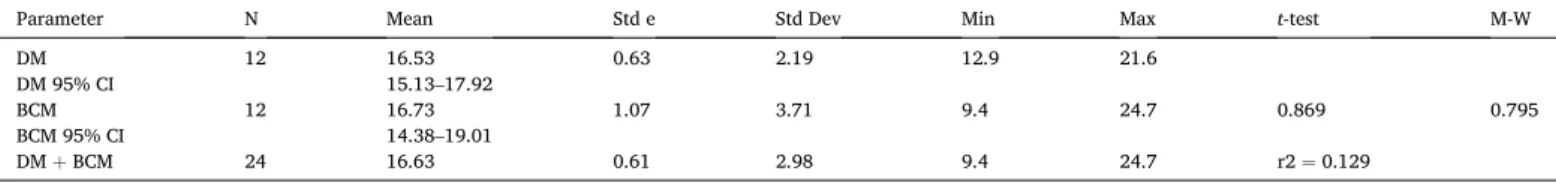
Summary statistics and t-test (parametric) and Mann-Whitney U (M-W, non-parametric) evaluation of directly measured (DM) and back calculated measurements (BCM) of Paleozoic atmospheric oxygen of halite fluid inclusion gas (Table 1), and their combined total for the Paleozoic.

Parameter N Mean Std e Std Dev Min Max t-test M-W

DM 12 16.53 0.63 2.19 12.9 21.6 DM 95% CI 15.13–17.92 BCM 12 16.73 1.07 3.71 9.4 24.7 0.869 0.795 BCM 95% CI 14.38–19.01 DM + BCM 24 16.63 0.61 2.98 9.4 24.7 r2 = 0.129 (A) 0.5 cm 1 cm (B)

Fig. 4. Two major types of halite. Plate A is an example of clear halite with few

to no fluid inclusions, and Plate B is cloudy halite replete with fluid inclusions and trails of inclusions (Davies, 2018). Halite type A is usually indicative of post-depositional recrystallization, whereas type B generally represents primary depositional halite.

Fig. 6B) and stretched (area i, Fig. 6B) due to compressional compaction forces (e.g., Popp and Kern, 2001), or they formed on a grain boundary surface due to migration forces (Fig. 5C, area ii). The Silurian Salina Formation is another example of the grain boundary migration process producing a multitude of secondary inclusions along the grain boundary (Fig. 6C, left side) as well as stretched inclusions (Fig. 6C, mid-section). In the Carboniferous Stewiacke Formation (Fig. 6D), we note a sec-ondary fluid inclusion trail along a grain boundary as well as secsec-ondary

cleavage cracks without inclusions (Fig. 6D, area i). It is not uncommon to find primary and well-preserved fluid inclusions in close proximity to deformed ‘tubed’ and other secondary inclusions (e.g., Figs. 5C, D, 6C). Our observations suggest that diffusion was probably minimal (Suppl. Fig. S1; cf. Zimmermann and Moretto, 1996) whereas the potential contribution of gas from inclusions generated by microfracturing may be a concern in atmospheric gas reconstructions based on halite fluid in-clusions. Deformational intra- and intercrystalline cracking may form

C

E

A

B

B

D

F

200 µm

200 µm

20 µm

200 µm

500 µm

200 µm

(i)

(ii)

Fig. 5. Major types of depositional petrographic features in modern and Paleozoic halite. Plate A shows primary depositional chevron fabric in modern halite, with

some early destruction of the fabric (arrow indicates area of dissolution). Area B corresponds to Plate B, a close-up of fluid inclusion trails and alternating dark and light bands of the chevron feature (A and B modified from Roberts and Spencer, 1995). Plate C shows primary, depositional fluid inclusions in halite from the upper Ordovician Red Heads Rapids Formation (area ii), and secondary fluid inclusions formed during grain boundary migration (area ii; Davies, 2018). Plate D shows primary, depositional fluid inclusions trails (arrow i) associated with chevron feature, and fluid inclusions with gas bubble (arrow i, ii) from the upper Silurian Salina Group (Davies, 2018). Plate E shows various fluid inclusions from a chevron feature in the upper McDonald Road Formation. Inclusions carry speckled oil (SO), clear oil (CO) and gas phase (between SO and CO, Shaver, 2018). Plate F shows primary, depositional fluid inclusions and trails in a chevron feature of the Salado Formation (modified from Knauth and Beeunas, 1986). (For interpretation of the references to colour in this figure legend, the reader is referred to the web version of this article.)

secondary inclusions filled with fluids as well as gas created during drilling of the core and dilatancy of the halite (Popp and Kern, 2001;

Schl´eder and Urai, 2005). Samples with fluid inclusions related to grain boundary migration should be removed from further analyses as they may cross contaminate original and primary fluid inclusion gas contents for reconstructing ancient atmospheres, or its results discarded from further interpretations.

4.3. Post-Depositional Recrystallization

Halite is highly susceptible to post-depositional recrystallization (dissolution-reprecipitation under shallow burial conditions and the presence of undersaturated waters/brines (Casas and Lowenstein, 1989;

Schreiber and El Tabakh, 2000). In the absence of fluids, halite may be preserved and archived at depth until extricated by the drilling of bore holes. Due to halite’s high solubility, the dissolution-reprecipitation process probably occurs under open system dynamics (cf. Brand and Veizer, 1980). In this process, the recrystallization of halite may be quite destructive in that it leads to the obliteration of possibly all primary and secondary fluid inclusions as evidenced by its generally ‘clear’ appear-ance (Fig. 4A) instead of the ‘cloudy’ appearance associated with depositional halite, which are generally replete with fluid inclusions (Fig. 4B).

5. Results

The extraction of gas trapped in inclusions from various substances, such as amber, ice, halite assumes that the gas has remained ‘locked’ away since its time of inception (Berner and Landis, 1988; Stolper et al., 2016; Blamey et al., 2016). The robustness of trapped gas faltered for inclusions in amber but remains intact for ice. Work on rock salt dem-onstrates that halite can be easily dissolved as well as readily altered during shallow post-depositional burial (Fig. 5A; Lowenstein and Har-die, 1985; Roberts and Spencer, 1995; Schreiber and El Tabakh, 2000), including drilling of a core and subsequent sample preparation (Roberts and Spencer, 1995). Despite the ease with which depositional features may be altered it just as readily allows for its identification. Conse-quently, halite with mostly depositional properties make it an attractive host material for burial of radioactive waste (Roedder and Bassett, 1981) and source for gas studies (Freyer and Wagener, 1970; Roedder, 1984). Primary fluid inclusions are usually associated with cumulates, chev-rons, cornets, fluid-inclusion trails and generally tend to be cubic in shape (Fig. 5B, C, D, E). In contrast, diagenetic or secondary inclusions formed during dilatancy and microfracturing may be smaller, square (ish), to round to elongated (Fig. 6). The close proximity of primary and secondary fluid inclusions may complicate results, at times, to obtain a

‘clean’ gas signal of just an original atmospheric origin from an indi-vidual crush(es) (e.g., Methods, Fig. 5C, E). Consequently, we try to get as many gas results from as many crushes as possible for each individual halite sample (cf. Messinian salt, Blamey et al., 2016).

5.1. Modern Halite: Key and Application to Ancient Counterparts

Modern halite with its extrinsic and intrinsic sedimentological/ geochemical information is one of the pillars that supports the concept of measuring atmospheric gas in ancient halite. The other pillar sup-porting this concept is the detailed screening of all material for depo-sitional, diagenetic and other post-depositional features (cf. Blamey and Brand, 2019). In this situation observation of primary features is rela-tively easy, and there is no need as in the modelling approach to rely extensively on proxies and hope that they have withstood the vicissi-tudes of deep-time diagenesis.

The presentation of modern halite information has been a corner-stone of our first publication (Blamey et al., 2016) and because of its importance to the whole concept it is worth summarizing the highlights (cf. Blamey and Brand, 2019). Information from modern non-marine and marine halite is supplemented by information of air trapped in capillary tubes and subsequently analysed in the same manner as halite and its fluid inclusions. A single primary non-marine or marine halite sample represents the global atmospheric gas and thus oxygen content irrespective of environmental and geographic setting. The best signal is ascertained by evaluation of its major and minor gas contents supple-mented by other elemental (e.g., Br) and isotopic compositions (e.g., strontium and argon). Microthermometry and the maximum homoge-nization temperatures are equally important in evaluating the burial regime and impact on halite fluid and gas composition. In addition, the back-calculated method measurements of gas contents (indirect proxy), specifically oxygen, is a great confirmatory tool of the directly measured oxygen content (direct proxy) in modern and deep-time halites.

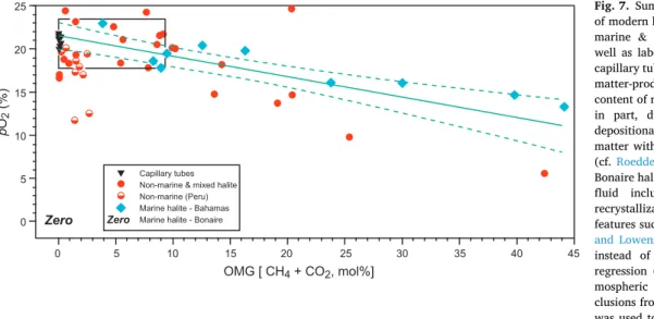
Fig. 7 is a compilation of the major components of the first concept pillar of gas contents in modern halite. The results encompass gas, also from capillary tubes of trapped lab gas, of non-marine halite from various global continental settings, and of marine halite from several environments sourced from the open ocean. Good analytical results are made possible by the sophisticated new instruments compared to those used by the pioneers in this field, Freyer and Wagener (1970). Each capillary tube and its gas content is crushed and analysed as a distinct entity, and the results of them cluster close about the expected modern atmospheric oxygen content, and the same applies to their combined low methane and carbon dioxide contents (Fig. 7). Saline brines, the source of non- and marine halites are full of organic matter and micro-organisms that may have an impact on the gas content of the ‘trapped’

C 200 µm 200 µm 200 µm A B 50 µm D (i)

Fig. 6. Major types of secondary features in Paleozoic halite. Plate A: Secondary

fluid inclusions are arranged in echelon cracks within the Ara Group halite. Plate B: Mixed and in close proximity are secondary (area i) and primary (area ii) fluid inclusions in the Red Head Rapids Formation halite (Davies, 2018). Plate C: grain boundary migration-formed (left side) and stretched (centre) fluid inclusions within the Salina Group (Davies, 2018). Plate D: secondary fluid inclusion arrays along cleavage crack and trans-granular cracks (area i; Shaver, 2018). (For interpretation of the references to colour in this figure legend, the reader is referred to the web version of this article.)

bubbles within the primary depositionally-formed fluid inclusions. Furthermore, gases in modern halite reflect their close association with halo-tolerant organisms present in saline brines (Casas and Lowenstein, 1989) and consequently the presence of biogenically-produced and consumed gas (e.g., Roedder, 1984), with a concomitant impact on the trapped oxygen. For example, this is exactly what we observe in the gas results of primary non-marine and marine halite (Fig. 7). This material with or without a directly measured result may be suitable for the advocated back calculation measurements method. Not all modern halite fulfills the criteria or need of primary preserved and adequate fluid inclusions. The results of gas from fluid inclusions of the non- marine halite from Peru for the most part are indicative of the ambient atmosphere (Fig. 7). However, with increasing water depth incorporation of air in fluid inclusions becomes problematic to the point of no air in fluid inclusions, if present at all. Only two crush results of material from Peru show the first stages of decreasing air in halite precipitated in increasing water depth. In addition, the marine halite sample from Bonaire gave no return of any air after crushing and analysis by mass spectrometry (Fig. 7). This relates to the nature of the material from Bonaire in that it was clear (cf. Fig. 4A) and lacked any discernable primary fluid inclusions. This suggests that shallow burial dissolution and reprecipitation obliterated any and all primary fabrics including fluid inclusions in the Bonaire sample (Fig. 4A; Lowenstein and Hardie, 1985; Roberts and Spencer, 1995; Schreiber and El Tabakh, 2000; Goldstein, 2001).

In summary, modern halites provide a key to identifying primary features in ancient and deep-time halite and thus, fluid inclusions with primary and ambient air including oxygen (cf. 4B). This trapped air in either non-marine or marine halite provides a global signal unfettered by local environmental impacts. The back-calculation measurement method (detailed below) provides for an additional and confirmatory source of results underpinning those garnered from direct measurements in fluid inclusions. The key for ancient halite is the preservation of primary features and their identification after detailed screening of physical and geochemical parameters (cf. Blamey and Brand, 2019).

5.2. Principle of Back-Calculated Measurements (BCM)

Atmospheric gas and oxygen were measured in gas bubbles trapped in fluid inclusions of modern halite from a number of marine and non- marine samples (Fig. 7, Table 1). This dataset was used to

demonstrate that directly measured gas concentrations and contents (DM) can be matched by those through the back calculation measure-ment method. A regression was placed over the gas results from the marine halite of the Bahamas (Fig. 7) to formulate a trend in oxygen content changes with increasing biologically-modified gas content. Evaluation of the gas components from fluid inclusions of the Bahamian halite give an intercept value of 21.63 ± 0.79% and 95% CI intercept values at 19.83% and 23.53%, which speak clearly to fact that any population should be able to resolve a global atmospheric oxygen value (Fig. 7, Supplementary StatsFigure 1, Appendix 3).

The regression of gas contents in fluid inclusions of marine and non- marine modern halite from Israel, Australia, United States and the Bahamas (Supplementary StatsFigure 2, Appendix 3) gives an intercept value of 21.41 ± 0.73% that is similar to the current oxygen content directly measured from halite fluid inclusions (20.29%), and compares well to that of the modern atmosphere (20.95%, Table 1). Considering the 95% confidence levels intercept values of 20.01 and 22.70% in-creases the veracity of the gas inclusion analyses used in the back calculation measurement method.

Statistical comparison of the average atmospheric oxygen contents from modern to Ediacaran halite have similar means with low standard errors (Table 2). Furthermore, the statistical analysis reveals no signif-icant difference (t-test and Mann-Whitney) between the two datasets at the 95% confidence level (p = 0.05, Table 2). Indeed, the robustness of the proposed back calculating measurement method for determining original oxygen contents in halite that were subjected to organic matter decomposition and concomitant CO2 and CH4 production and O2

con-sumption, will be tested and compared on all Ediacaran to Permian study material (Table 2; Figs. 8, 9; Appendices 3, 4, 5).

5.3. Gas Results of Halite

We evaluate both new (Appendix 1) and old datasets (Appendix 2) in this section and present them in chronological order for the Paleozoic, plus results from the latest Ediacaran. Data points for the direct mea-surement (DM) of original oxygen contents are confined, in part, by an upper limit of a combined 10% for CO2 and CH4 (Blamey and Brand, 2019), and supported by other physical features and geochemical pa-rameters, among them appropriate bromine contents, homogenization temperatures and consistent argon isotope values (Blamey and Brand, 2019). In contrast, back calculated measurements (BCM) will be

25 20 15 10 5 0 0 Zero Zero 5 10 Capillary tubes 15 20 25 30 35 40 45 OMG [ CH4 + CO2, mol%] p O2 (%)

Non-marine & mixed halite Non-marine (Peru) Marine halite - Bahamas Marine halite - Bonaire

Fig. 7. Summary of fluid inclusion gas analysis

of modern halite from various marine and non- marine & mixed environmental localities, as well as laboratory atmospheric gas trapped in capillary tubes (cf. Blamey et al., 2016). Organic matter-produced gas (OMG) is the combined content of methane and carbon dioxide formed, in part, during a) formation and b) post- depositional decomposition of trapped organic matter within the fluid inclusions of the halite (cf. Roedder, 1984; Blamey and Brand, 2019). Bonaire halite produced no gas due to its lack of fluid inclusions suggesting shallow burial recrystallization and obliteration of primary features such as fluid inclusions (Fig. 4A; Casas and Lowenstein, 1989); thus the use of ‘zero’ instead of a symbol. Ordinary least-squares regression (including 95% CI intervals) of at-mospheric oxygen versus OMG in fluid in-clusions from the marine halite of the Bahamas was used to formulate the base parameters for the back calculation measurement method (see Appendix 3, Supplementary StatsFigures 1 and 2 for computer generated figures and statistical information). This allows for the determination of the ‘original’ primary oxygen, methane and carbon dioxide contents of trapped gas within cumulate, cornet and chevron fabrics of ancient marine and non-marine halite modified by post-depositional biogeochemical processes (organic matter decomposition).

determined using all gas results for a specific formation consisting of one or several sets of gas analyses spanning the full range of CO2 and CH4

contents (cf. modern counterparts), but excluding those results clearly linked to grain boundary migration ‘leakage’ formation and origin (e.g., Salt Range** results, Table 1) and cross contamination.

5.3.1. Ediacaran

The gas results for the Ediacaran were part of the Blamey et al. (2016) study dealing with extracting oxygen contents from the Tonian

(815 Ma) Brown Formation of Australia. The 545 Ma old Hongchunping halite of China records a direct oxygen value of 17.4% (DM) and a comparable 17.7% for the back calculated one (BCM; Table 1). They seem to be reasonable for salt that has formation temperatures ranging from 16 to 39 ◦C (Meng et al., 2011; Table 1). A similar DM value of

17.6% for oxygen is also derived from fluid inclusion gas analyses of the Salt Range formation of Pakistan (Table 1), and a comparable BCM value of 16.9%. In contrast are some excluded results from the Salt Range formation that give an average oxygen value of 26.4% (Table 1) and are more consistent with fluid inclusions associated with air contamination due to grain-boundary migration. Nevertheless, the similarity in both DM and BCM atmospheric oxygen values of halite from two geograph-ically separated localities (China and Pakistan) provides additional support to their primary nature (cf. Blamey et al., 2016; Blamey and Brand, 2019).

5.3.2. Cambrian

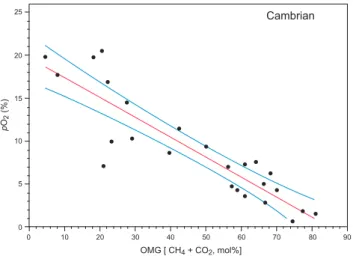
Gas results are abundant for the earliest Cambrian halite from the Ara Group of Oman, but sparse with only two results satisfying the screening constraints (Blamey and Brand, 2019) needed for primary values (Fig. 8). Nevertheless, the two ‘primary’ results give an average value of 18.8% (DM), and are supplemented with results of 19.8% at 0% OMG, and 18.7% at 5% OMG back calculated for all the extracted gas results (BCM, Table 1, additional detail in Supplementary StatsFigure 3, Appendix 3). The Br content of 145 ppm is reasonable for halite formed in the middle of the evaporation sequence (x11 to x65 seawater con-centration, McCaffrey et al., 1987). Fortunately, gas from echelon-crack fluid inclusions was not picked up during the gas extraction process (Fig. 6A). Overall, the Cambrian results continue the rise of atmospheric oxygen observed since the Ediacaran (5.3.1) and Tonian (Blamey et al., 2016).

5.3.3. Ordovician

The mid Ordovician halite from the Majiagou Formation of China is texturally and geochemically well-defined suggesting good preservation (Ran et al., 2012; Hu et al., 2014). Its halite-based atmospheric oxygen content of 15.4% and back calculated measurement content of 15.8% are lower than the average measured for the latest Ediacaran through Cambrian with 18.0% (Table 1, Suppl. Fig. S3), while maintaining reasonable marine Br contents and homogenization temperatures.

The gas results from the halite of the upper Ordovician Red Head Rapids Formation of the Hudson Bay Basin (Fig. 3) document complex depositional and post-depositional conditions (Fig. 9). The gas results can be divided into three clusters (cf. Table 1), 1) representing primary gas contents (regression field, Fig. 9; Fig. 5C), 2) diagenetically modified gas contents (field i, Fig. 9; Fig. 6B), and 3) gas associated with fluid inclusions ‘formed’ of contaminated air during grain boundary migra-tion (field ii, Fig. 9). The directly measured original oxygen content of 15.7% (DM) is similar to the back calculated value of 16.6% (BCM). Results in field i (Fig. 9; 7.4%, Table 1) probably represent halite and gas inclusions formed in the relatively deeper and oxygen-reduced water column (cf. Peru, Fig. 7). Another batch of results represents consider-ably higher gas contents of 22.2% formed during grain boundary migration and associated with cross-contamination with ambient air (field ii, Fig. 9; Fig. 5C; Table 1). Overall, the fluid inclusion gas results from the Red Head Rapids Formation cover the end-Ordovician.

5.3.4. Silurian

Gas results of the Silurian show some of the greatest variation in oxygen contents measured in halite during the early Paleozoic. The Mallowa salt (Carribuddy Group) of the Canning Basin (Australia) comes in with a low oxygen content of 12.9% (DM) and comparable 14.3% using the BCM method (Table 1, Suppl. Fig. S4). This is followed by a drastic increase in oxygen content during Salina A2 time up to 21.6% (DM) and BCM value of 24.7% (Table 1, Fig. 5D, Suppl. Fig. S5A). In addition, extensive grain boundary migration produced some ‘leaked’

25 20 15 10 5 0 0 10 20 30 40 50 60 70 80 90 p O2 (%) Cambrian OMG [ CH4 + CO2, mol%]

Fig. 8. Back Calculated Measurement (BCM) method of atmospheric oxygen

and methane plus carbon dioxide (OMG) gas in fluid inclusions measured in the Cambrian Ara Group halite from Oman (cf. Blamey et al., 2016). Least squares regression and 95% CI overlain on all results gives an intercept of 19.80% and error of 1.29 for oxygen at 0% OMG (Table 1; see Appendix 3, Supplementary StatsFigure 3 for computer generated figure and statistical information).

25 30 Upper Ordovician 20 15 10 5 0 0 10 20 30 40 50 60 70 80 90

OMG [ CH4 + CO2, mol%]

p

O2

(%)

ii

i

Fig. 9. Back calculated measurement (BCM) method of atmospheric oxygen

and methane plus carbon dioxide (OMG) gas in fluid inclusions measured in upper Ordovician Red Head Rapids Formation halite from northern Ontario (Fig. 3). Least squares regression and 95% CI covers the majority of data with an intercept of 16.6% and an error of 0.7 for oxygen at 0% OMG (Table 1). Other results fall into two fields, with field (i) characterizing results of halite that probably formed in ‘deeper’ waters and are thus low to devoid of oxygen (cf. Peru halite, Fig. 7). Field (ii) represents fluid inclusions and contents formed and possibly cross-contaminated with ambient air during post-depositional grain boundary migration. Back calculation measurement results of other Paleozoic halites are in Appendix 4. (For interpretation of the references to colour in this figure legend, the reader is referred to the web version of this article.)

oxygen values of 20.4% similar to that of modern air and halite (Table 1,

Fig. 6C, Supp. Fig. S5A, field i). Subsequently, by Salina B time atmo-spheric oxygen contents had dropped back down to about 16.5% (DM) and 19.8% (BCM; Table 1, Supp Fig. S5B), to levels reflecting those of Cambrian-Ordovician times.

5.3.5. Carboniferous

By the lower Carboniferous (Visean) atmospheric oxygen levels had stabilized at about 15.0% (DM) and 15.5% (BCM) after the tumultuous Silurian (Table 1, Supp. Fig. S6). This atmospheric oxygen consistency continued through the Stewackie Formation (15.2%) and upper McDo-nald Road Formation (15.5%) of the Maritimes Basin (Table 1, Supp. Fig. S7). The Stewackie halite shows evidence of fracture-related fluid inclusion trails (Fig. 6D), while the upper McDonald halite is replete with gas-charged fluid inclusions (centre Fig. 5D, Supp Fig. S7A) sur-rounded by various fluid inclusions trapping both speckled and clear (oil) hydrocarbons (SO, CO, Fig. 5D). Some other areas within the McDonald halite have fluid inclusions with oxygen contents mimicking that of hydrocarbon-charged air (Supp. Fig. S7B).

5.3.6. Permian

The Permian Salado halite of the Permian Basin is replete with pri-mary chevron structures which contain abundant fluid inclusion trails. Some of the best-preserved atmospheric oxygen content comes in at 24.2% (BCM) and 16.9% (DM) to 14.5% (BCM) during a short time interval just preceding the end Permian mass extinction (Table 1, Supp. Fig. S8; e.g., Brand et al., 2016; Jurikova et al., 2020). It appears that atmospheric oxygen content is on the decline concurrent with a decrease in faunal abundance. The classical oxygen results of the Zechstein halite are included in Table 1, and with an average of 14.7% are similar to results obtained from the Salado Formation. Although the averages are similar, the great uncertainty is in all the measurements that range from a low of 2.4% to a high of 43.3% for the Zechstein halite (Table 1). This great error in precision is a reflection of the old technology (instrument and sample preparation; Freyer and Wagener, 1970), which since then has been overcome by a new and improved low-temperature crushing method and high-precision mass spectrometric analysis (cf. Blamey, 2012).

6. Discussion

From the melange of models and atmospheric trends proposed over the decades, we have chosen to compare our results to those of the COPSE (Bergman et al., 2004), GEOCARBSULF (Berner, 2009), and GEOCARBSULFOR (Krause et al., 2018) models, and for good measure the lower and upper limits of the Wildfire Window (Glasspool and Scott, 2010). Furthermore, since there is no statistical difference between our directly measured (direct proxy) data and back calculated measure-ments (Indirect proxy, Table 2), we will treat them as a single entity in the associated figure (Fig. 10) and its subsequent evaluation.

6.1. General Evaluation

Several papers recently challenged the infallibility of the RSE and RSI concepts that form the basis for their respective models (e.g., COPSE, GEOCARBSUL and GEOCARBSULFOR) (Algeo and Liu, 2020; Bennett and Canfield, 2020). Everything from a re-examination to calibration of the base parameters is called for in those publications. Another concept of utmost importance is the global aspect of sedimentary rock – based RSE and RSI parameters in an attempt to ‘harmonize’ the divergent oxygen trends between the two most prominent models, the COPSE and GEOCARBSUL (Zhang et al., 2018; Mills et al., 2019). It is postulated that by “…changing the input carbonate δ13_{C within the geologic data}

range, we can maintain a low O2 level in GEOCARBSULF…” (Zhang et al., 2018, p. 569) for the early Paleozoic. They go on to state that “…δ13C of brachiopods exhibit substantial regional heterogeneity…”

and is the cause for a poorly known global Paleozoic carbonate δ13_C

values and thus atmospheric oxygen. Brand et al. (2015) clearly demonstrated the high carbon isotope composition variability of low- and mid-latitude modern brachiopods. The δ13_{C values of modern}

bra-chiopods range from − 1.76 to +3.60‰ (Brand et al., 2015), which is mirrored by the variability observed in all Devonian brachiopods (− 0.9 to +3.9‰, van Geldern et al., 2006), and is slightly lower than that observed in all Carboniferous counterparts (+1.0 to 5.5‰, Grossman et al., 2008). The robustness of these results is not in doubt, since the respective authors used detailed investigations to select the best pre-served material. Instead, it is the paucity of material covering the whole spectrum of geography-specific to species-specific variation observed in low to mid latitude marine settings (Brand et al., 2015; Ullmann et al., 2017). This speaks directly to the question of ‘how global are the geochemical signals from individual biogenic and abiogenic populations and/or carbonate, pyrite sedimentary units? Krause et al. (2018)

modelled the Paleozoic atmospheric oxygen using the latest carbonate carbon isotope and pyrite sulfur isotope data, while Large et al. (2019)

used RSEs such as Se and Co of sedimentary pyrite to trace the atmo-spheric oxygen of the Paleozoic. The end results is no agreement in the atmospheric oxygen trend for the Paleozoic between these two models (cf. Fig. 2); again why?

The answer is obvious, currently we know that oxygen in air trapped within primary halite fluid inclusions represents a global atmospheric signature (cf. Fig. 7; Blamey and Brand, 2019), and the same holds true for strontium isotopes in marine sedimentary units representing seawater chemistry (e.g., Zaky et al., 2019). So, the question of the ‘Global aspect’ of RSEs and RSIs in addition to their calibration should be addressed before atmospheric gas modelling research moves forward (cf., Algeo and Liu, 2020; Bennett and Canfield, 2020). More inter- sample and results calibration and comparison are needed for model-ling of ancient atmospheric gas (oxygen, carbon dioxide, etc.) levels based on RSEs, RSIs and halite (cf. Steadman et al., 2020).

6.2. Paleozoic Atmospheric Oxygen

Fig. 10 shows the results of the three datasets (e.g., Berner, 2001), as

Age (Ma)

C

D

S

O

E

P

Tr

C

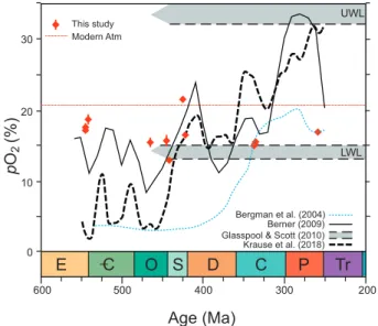
Glasspool & Scott (2010) Krause et al. (2018) LWL Bergman et al. (2004)

p

O

(%)

Fig. 10. Summary compilation of Paleozoic atmospheric oxygen measured in

fluid inclusions trapped in deep-time halite (Table 1). Superimposed are the results and trends modelled with the COPSE (Bergman et al., 2004), GEO-CARBSULF (Berner, 2009) and GEOCARBSULFOR (Krause et al., 2018) models. Also, the lower (LWL) and upper (UWL) ‘wildfire’ limits (Lenton et al., 2018;

Glasspool and Edwards, 2004) and the ‘modern’ atmospheric oxygen content are depicted in the figure. The symbols of the measured oxygen (DM and BCM) contents in the fluid inclusions of halite represent the total error (Table 1).

well as the lower and upper wildfire limits, the ‘wildfire window’, based on documented charcoal (inertinite) in the geologic record (Scott and Glasspool, 2006; Glasspool and Scott, 2010; Lenton et al., 2018). The Ediacaran-Cambrian and Ordovician-Silurian transitions lend them-selves to comparisons of limited time constrain but representing wide geographical variation. In the case of the Ediacaran-Cambrian we have invariant atmospheric oxygen results from China, Pakistan and Oman (Table 1).

Our average atmospheric oxygen contents ranging from 17.4 to 19.3% for the late Ediacaran to early Cambrian are in agreement with generally predicted levels, and are ‘sandwiched’, by those of the pyrite- RSE model (Sup Fig. S9), but are higher than those predicted by the COPSE, GEOCARBSULF and GEOCARBSULFOR models (Fig. 10). These elevated oxygen contents level down and off into the mid Ordovician with 15.6% pO2, which is right on mark with the level predicted by the

pyrite-RSE model but well above the other prominent models (Fig. 10, Sup. Fig. S9). Our late Ordovician (16.2%) – early Silurian (13.7%) oxygen contents are matched again by the levels proposed by the pyrite- RSE model transect the GEOCARBSULF trend, but are slightly higher than the GEOCARBSULFOR trend and continue to be significantly higher than those predicted by the COPSE model (Fig. 10).

The mid to late Silurian oxygen contents spike upward to a high of 23.2% followed by a gradual decrease to 18.2% (Fig. 10). These values and trends appear to have some semblance of compatibility with those of the GEOCARBSULF and GEOCARBSULFOR model trends. The Visean (early Carboniferous) atmospheric oxygen values (15.3, 15.2, 15.7%) are similar or close to those proposed by the pyrite-RSE (Sup. Fig. S9) and COPSE, GEOCARBSULF models (Fig. 10). For the late Permian, at-mospheric oxygen levels continue at about 15.7%, a level observed during the Visean, and are in line with the average of the classical results of Freyer and Wagener (1970) for the latest Permian with 14.7%. Un-fortunately, their methodology did not have the required precision for a robust reconstruction of deep-time atmospheric oxygen levels (Table 1; Appendix 2).

At this time, we have no halite-sourced oxygen results that corre-spond to the high atmospheric oxygen levels proposed for the Devonian, Carboniferous and Permian intervals postulated by the GEOCARBSUL and GEOCARBSULFOR models. Apart from the pyrite-RSE model of

Large et al. (2019), agreement between the various models and proposed atmospheric oxygen levels is low. Our halite dataset supports a relatively constant atmospheric oxygen level of 16.6% (0.6% SE, 2.9 SD) for the Paleozoic, and thus, events associated with fluxes in the hydrosphere, biosphere must look for other causal sources.

7. Conclusions

Halite material from ten Paleozoic units/formations ranging from the early Cambrian to late Permian, supplemented by two from the latest Ediacaran, was tested and analysed for its gas content in fluid inclusions. Fluid inclusions evaluated in this study encompass the full spectrum of primary to diagenetic to syn- to post-depositional processes and the concomitant impact on inclusion gas contents. The results suggest and support the following conclusions:

1) Primary halite from modern to Ediacaran settings contain atmo-spheric gas suitable for determining the oxygen content,

2) directly measured atmospheric oxygen contents of halite are statis-tically indistinguishable from those derived with the back calcula-tion measurement method,

3) summary of all measurements of oxygen in gas bubbles trapped in primary fluid inclusions suggest that atmospheric oxygen varied from: a) 17. 4% during the late Ediacaran, b) 19.3% during the early Cambrian, c) 15.6% during the mid Ordovician, d) 16.2% during the late Ordovician, e) 13.6% during the early Silurian, f) 23.2% and then 18.2% during the mid-late Silurian, g) 15.3% during the early

Carboniferous, h) 15.5% during the Visean, and finally, i) about 15.7% during the late Permian,

4) in contrast to the various models, our combined directly and back calculated measured atmospheric oxygen results from primary halite fluid inclusions suggest a relatively near-constant level at about 16.5% (±0.6 SE, ±2.2 SD) for Paleozoic atmospheric oxygen.

Declaration of Competing Interest The authors declare no conflict of interest. Acknowledgements

We thank Dr. Feifei Zhang for inviting us to contribute to the special issue on the oxygen content of the Paleozoic atmosphere. A special thank you to the three reviewers and editors who made sure that we honed our manuscript and its content. Thanks to Mike Lozon (Brock University) for drafting the many versions of the figures, and Dr. Robert Linnen (Uni-versity of Western Ontario) for access to his microthermometry set-up. U. Brand acknowledges the Natural Science and Engineering Research Council of Canada for financial support (NSERC Discovery Grant 2015- 05196), and N. Blamey thanks the University of Western Ontario for financial support. A. Davis and K. Shaver acknowledge financial support of Brock University (teaching assistantships, a Dean of Graduate Studies Spring Research scholarship) and scholarships from the Ontario Grad-uate and Queen Elizabeth II GradGrad-uate Programs.

Appendix A. Supplementary data

Supplementary data to this article can be found online at https://doi. org/10.1016/j.earscirev.2021.103560.

References

Algeo, T.J., Ingall, E., 2007. Sedimentary Corg:P ratios, paleocean ventilation, and Phanerozoic atmospheric pO2. Palaeogeogr. Palaeoclimatol. Palaeoecol. 256,

130–155.

Algeo, T.J., Liu, J., 2020. A re-assessment of elemental proxies for paleoredox analysis. Chem. Geol. 540, 119549.

Amthor, J.E., Grotzinger, J.P., Schr¨oder, S., Bowring, S.A., Ramezani, J., Martin, M.W., Matter, A., 2003. Extinction of Cloudina and Namacalathus at the Precambrian- Cambrian boundary in Oman. Geology 31, 431–434.

Arvidson, T.J., Mackenzie, F.T., Guidry, M.W., 2013. Geologic history of seawater: a MAGic approach to carbon chemistry and ocean ventilation. Chem. Geol. 362, 287–304.

Beerling, D.J., Lake, J.A., Berner, R.A., Hickey, L.J., Taylor, D.W., Royer, D.L., 2002. Carbon isotope evidence implying high O2/CO2 ratios in the Permo-Carboniferous

atmosphere. Geochim. Cosmochim. Acta 66, 3757–3767.

Benison, K.C., Goldstein, R.H., 2000. Sedimentology of ancient saline pans: an example from the Permian Opeche Shale, Williston Basin, North Dakota, U.S.A. J. Sediment. Res. 70, 159–169.

Bennett, W.W., Canfield, D.E., 2020. Redox-sensitive trace metals as paleoredox proxies: a review and analysis of data from modern sediments. Earth-Sci. Rev. 204, 103175. Bergman, N.M., Lenton, T.M., Watson, A.J., 2004. COPSE: a new model of

biogeochemical cycling over Phanerozoic time. Am. J. Sci. 304, 397–437. Berkner, L.V., Marshall, L.C., 1965. On the origin and rise of oxygen concentration in the

Earth’s atmosphere. J. Atmos. Sci. 22, 225–261.

Berner, R.A., 1987. Models for carbon and sulfur cycles and atmospheric oxygen: application to Paleozoic history. Am. J. Sci. 287, 177–196.

Berner, R.A., 1991. A model for atmospheric CO2 over Phanerozoic time. Am. J. Sci. 291,

339–376.

Berner, R.A., 1994. GEOCARB II: a revised model of atmospheric CO2 over Phanerozoic

time. Am. J. Sci. 294, 56–91.

Berner, R.A., 2001. Modelling atmospheric O2 over Phanerozoic time. Geochim.

Cosmochim. Acta 65, 685–694.

Berner, R.A., 2006a. GEOCARBSULF: a combined model for Phanerozoic atmospheric O2

and CO2. Geochim. Cosmochim. Acta 70, 5653–5664.

Berner, R.A., 2006b. Inclusion of the weathering of volcanic rocks in the GEOCARBSULF model. Am. J. Sci. 306, 295–302.

Berner, R.A., 2009. Phanerozoic atmospheric oxygen: new results using the GEOCARBSULF model. Am. J. Sci. 309, 603–606.

Berner, R.A., Canfield, D.E., 1989. A new model for atmospheric oxygen over Phanerozoic time. Am. J. Sci. 289, 333–361.

Berner, R.A., Kothavala, Z., 2001. GEOCARB III: a revised model of atmospheric CO2