HAL Id: hal-01862645
https://hal.archives-ouvertes.fr/hal-01862645
Submitted on 27 Aug 2018
HAL is a multi-disciplinary open access
archive for the deposit and dissemination of
sci-entific research documents, whether they are
pub-lished or not. The documents may come from
teaching and research institutions in France or
abroad, or from public or private research centers.
L’archive ouverte pluridisciplinaire HAL, est
destinée au dépôt et à la diffusion de documents
scientifiques de niveau recherche, publiés ou non,
émanant des établissements d’enseignement et de
recherche français ou étrangers, des laboratoires
publics ou privés.
African Rift from S travel time tomography
Chiara Civiero, Saskia Goes, James Hammond, Stewart Fishwick,
Abdulhakim Ahmed, Atalay Ayele, Cécile Doubre, Berhe Goitom, Derek Keir,
J. Michael Kendall, et al.
To cite this version:
Chiara Civiero, Saskia Goes, James Hammond, Stewart Fishwick, Abdulhakim Ahmed, et al..
Small-scale thermal upwellings under the northern East African Rift from S travel time tomography. Journal
of Geophysical Research : Solid Earth, American Geophysical Union, 2016, 121 (10), pp.7395 - 7408.
�10.1002/2016JB013070�. �hal-01862645�
Small-scale thermal upwellings under the northern
East African Rift from
S travel time tomography
Chiara Civiero1, Saskia Goes1, James O. S. Hammond2, Stewart Fishwick3, Abdulhakim Ahmed4,5, Atalay Ayele6, Cecile Doubre7, Berhe Goitom8, Derek Keir9,10, J. Michael Kendall8, Sylvie Leroy4, Ghebrebrhan Ogubazghi11, Georg Rümpker12, and Graham W. Stuart13
1
Department of Earth Science and Engineering, Imperial College London, London, UK,2Department of Earth and Planetary Science, Birkbeck, University of London, London, UK,3Department of Geology, University of Leicester, Leicester, UK, 4
Sorbonne Universités, UPMC Univ Paris 06, UMR 7193, Institut des Sciences de la Terre Paris, Paris, France,5Seismological and Volcanological Observatory Center, Dhamar, Yemen,6Institute of Geophysics, Space Science and Astronomy, Addis
Ababa University, Addis Ababa, Ethiopia,7Institut de Physique du Globe, Université de Strasbourg/EOST, Strasbourg, France,8School of Earth Sciences, University of Bristol, Bristol, UK,9National Oceanography Centre Southampton, University
of Southampton, Southampton, UK,10Dipartimento di Scienze della Terra, Università degli Studi di Firenze, Florence, Italy,
11Eritrea Institute of Technology, Asmara, Eritrea,12Institute of Geosciences, Goethe-University Frankfurt, Frankfurt,
Germany,13School of Earth and Environment, University of Leeds, Leeds, UK
Abstract
There is a long-standing debate over how many and what types of plumes underlie the East African Rift and whether they do or do not drive its extension and consequent magmatism and seismicity. Here we present a new tomographic study of relative teleseismic S and SKS residuals that expands the resolution from previous regional studies below the northern East African Rift to image structure from the surface to the base of the transition zone. The images reveal two low-velocity clusters, below Afar and west of the Main Ethiopian Rift, that extend throughout the upper mantle and comprise several smaller-scale (about 100 km diameter), low-velocity features. These structures support those of our recent P tomographic study below the region. The relative magnitude of S to P residuals is around 3.5, which is consistent with a predominantly thermal nature of the anomalies. The S and P velocity anomalies in the low-velocity clusters can be explained by similar excess temperatures in the range of 100–200°C, consistent with temperatures inferred from other seismic, geochemical, and petrological studies. Somewhat stronger VSanomalies below Afar than west of the Main Ethiopian Rift may include an expression of volatiles and/or melt in this region. These results, together with a comparison with previous larger-scale tomographic models, indicate that these structures are likely small-scale upwellings with mild excess temperatures, rising from a regional thermal boundary layer at the base of the upper mantle.1. Introduction
East African extension and its accompanying volcanic and tectonic activity (Figure 1a) are commonly asso-ciated with one or more mantle plumes rising below the region [e.g., Burke, 1996; Ebinger and Sleep, 1998]. Indeed, global- and continental-scale models have consistently found strong low-velocity regions below the continent, both in the shallow and deep mantle [e.g., Fishwick, 2010; Ritsema et al., 1999]. There is how-ever much debate about whether the deeper structure connects with that of the upper mantle.
Some groups have advocated the existence of a single strongly tilted upwelling rooted in the African Large Low-Shear-Velocity Province and rising tofill most of the upper mantle from Tanzania to the Red Sea. This is consistent with the pervasive low velocities in the region [Hansen et al., 2012; Ritsema et al., 1999], broad-scale uplift [Daradich et al., 2003], and a consistent pattern of along-rift directions of fast seismic anisotropy [e.g., Gao et al., 2010; Hammond et al., 2014; Kendall et al., 2005; Montagner et al., 2007]. However, others have pro-posed the existence of at least two separate branches from the lower into the upper mantle, based on more detailed tomographic imaging [Chang and Van der Lee, 2011; Debayle et al., 2001; Koulakov, 2007; Montelli et al., 2004b], variations in lava chemistry [Furman et al., 2004; George et al., 1998; Pik et al., 2006; Rogers et al., 2000], and modeling of the geoid and the evolution of magmatism [Lin et al., 2005]. A recent P tomo-graphic study we performed below the northern East African Rift [Civiero et al., 2015] combined regional seis-mic data sets across the region to obtain resolution to the base of the transition zone and revealed even smaller structures (scales ~100 km) extending across the depth of the upper mantle. We proposed these to
Journal of Geophysical Research: Solid Earth
RESEARCH ARTICLE
10.1002/2016JB013070
Key Points:
• S wave tomography shows multiple upper mantle upwellings below the northern East African Rift as previously proposed using P tomography • Both S and P anomalies are consistent
with a dominantly thermal signature of 100-200° excess temperature • The complex transition zone structure
may well connect to lower mantle roots revealed in large-scale tomography Supporting Information: • Supporting Information S1 Correspondence to: S. Goes, s.goes@imperial.ac.uk Citation:
Civiero, C., et al. (2016), Small-scale thermal upwellings under the northern East African Rift from S travel time tomography, J. Geophys. Res. Solid Earth, 121, 7395–7408, doi:10.1002/ 2016JB013070.
Received 7 APR 2016 Accepted 2 OCT 2016
Accepted article online 6 OCT 2016 Published online 21 OCT 2016
©2016. The Authors.
This is an open access article under the terms of the Creative Commons Attribution License, which permits use, distribution and reproduction in any medium, provided the original work is properly cited.
be small-scale upwellings rising from a zone of (ponded) hot material at the base of the upper mantle. Such small-scale structures are consistent with those imaged by previous tomographic studies with resolution down to about 400 km depth [Bastow et al., 2005; Bastow et al., 2008; Hammond et al., 2013] and also with proposed interpretations of strongly variable isotopic characteristics of lava along the rift [Furman et al., 2006; Meshesha and Shinjo, 2008].
Here we present a complementary tomographic inversion of relative S and SKS travel times to (a) assess robustness of the structure revealed by our P tomography [Civiero et al., 2015], which we refer to as NEAR-P15, and (b) more importantly, to further constrain the thermal and/or chemical nature of the structures.
2. Method
2.1. Data
This study uses broadband recordings of teleseismic S and SKS wave phases from 379 stations across east-ern Africa, from Malawi to Eritrea, and the Arabian Peninsula (i.e., all those shown in Figure 1b). The seis-mic stations belong to 16 multinational projects and overlap spatially and/or temporally in our region of interest (see supporting information). There has been some confusion in the literature about the resolving capability of the different generations of tomographic models in the northern East African Rift [e.g., Reed et al., 2016]. Early studies used stations in and around the Main Ethiopian Rift, resolving P and S wave velocities in the top 300–400 km [Bastow et al., 2005; Benoit et al., 2006; Bastow et al., 2008]. The data set was extended into Afar and Eritrea by Hammond et al. [2013], who focused their interpretation on Figure 1. (a) Tectonic map of the East African Rift, showing the presence of two topographic domes, the main faults of the rift system (in brown), with the Main Ethiopian Rift (MER) cutting through the Ethiopian Plateau, and a Western (WB) and Eastern Rift Branch (EB) around the Kenyan Plateau. Holocene volcanoes (in orange) largely concentrate along the rift zone (Smithsonian Volcanism Program 2013). The black rectangle delineates the area of interpretation. (b) Distribution of all stations used in this study, symbol coded according to their network. Network and station information can be found in Table S1 in the supporting information. (c) Distribution of earthquake sources used for the S-SKS tomography. Source-receiver distances shown by the circles on the inset are from the center of the black rectangle in Figures 1a and 1b.
the top 400 km in relation to rifting in Afar. However, due to the increased aperture of their seismic array resolution, particularly, the S wave model, due to the inclusion of significant SKS data, was good to depths of ~600 km. As a result, the Hammond et al. [2013] model was used to compare against images of transition-zone discontinuity structure in Thompson et al. [2015]. The most recent models of Civiero et al. [2015] and this study have extended the data significantly further, including data from Saudi Arabia to Malawi. As shown in Civiero et al. [2015] and Figure S8 in the supporting information this sub-stantially increases crossing rays in and around the transition zone and thus allows us to confidently inter-pret seismic velocity models to the base of the transition zone.
We pick arrival times from 590 earthquakes of magnitude mb≥ 5.5, ranging in epicentral distance from 30°
to 130° (30°–90° for S waves and 90°–130° for SKS waves). The azimuthal and distance coverage provided by the selected earthquakes is displayed in Figure 1c. After applying a 0.04–0.15 Hz band-pass Butterworthfilter, S picking was performed on the transverse component, to minimize the effect of P, P-S, and S-P conversions, while SKS picking was done on the radial component, as it is dominated by SV energy. Final picks and relative arrival times were determined using the multichannel cross-correlation method of VanDecar and Crosson [1990], in a 12 s window around the initial pick. We deleted all picks with cross-correlation coefficients <0.80 from our analysis. In total, we retain 16,569 travel time picks, divided into 8730 and 7839 S and SKS wave phases, respectively. The mean RMS uncertainty in the delay times, based on the number of picks rather than on cross-correlation pairs for each event [Tilmann et al., 2001], is 0.38 s with a standard deviation of 31 s (S wave mean RMS uncertainty = 0.34 s with standard deviation = 0.28 s and SKS wave mean RMS uncertainty = 0.43 s with standard deviation = 0.33 s). The range of S and SKS travel time residuals is about ±10 s. To reduce the effect of a few higher outliers, residuals larger than 3.0 standard deviations are downweighted iteratively in the inversion [Huber, 1981]; 827 rays end up downweighted, i.e., about 5% of the data.
2.2. Tomographic Inversion
The data are inverted using the teleseismic travel time inversion method of VanDecar et al. [1995], with the same scheme as in our previous P wave tomographic analysis [Civiero et al., 2015], which has been used and described in numerous previous studies [e.g., Hammond et al., 2013; Ritsema et al., 1998; Schimmel et al., 2003; Wolfe et al., 1997; Wolfe et al., 2009]. We use ray theory and perform a linear inver-sion; both assumptions should not have a substantial effect on the shape of the anomalies but may somewhat affect amplitudes [e.g., Bastow et al., 2005; Montelli et al., 2004a; Peter et al., 2009]. There is insufficient information on crustal structure below the whole network to correct the data for station sta-tics, so we solve for station (and event) corrections as part of the inversion. We use exactly the same para-meterization as in NEAR-P15, with an inner grid below the stations of 0.5°/0.4° node spacing in latitude/longitude and 50 km in depth, extending down to 1500 km, and an outer grid with 1° node spa-cing and 100 km depth spaspa-cing extending to 28°N–25.40°S in latitude, 25°E–57.20°E in longitude, and 2000 km in depth, to avoid mapping outside structure into our region of interest.
We regularize the model by suppressing spatial and curvature gradients (smoothing andflattening), as well as, in part of the cases, by damping toward a 3-D reference structure. We first investigate the trade-off between the RMS residual reduction and RMS model roughness for different combinations of smoothing andflattening to choose a preferred model that fits the data well, i.e., within a residual reduc-tion that can be justified by the estimated noise level. We obtain the same preferred regularization para-meters for our final model (which we will call NEAR-S16), as for NEAR-P15, although they were determined independently. Preferredflattening and smoothing factors are 4800 and 153,600, respectively (Figure 2).
In most previous travel time inversions for the region, a 1-D starting model was used (i.e., zero anomaly, as the relative travel time method has no sensitivity to 1-D structure) and no explicit damping to it was performed [Bastow et al., 2005; Bastow et al., 2008; Hammond et al., 2013]. However, teleseismic travel time tomography provides relatively poor resolution of the crustal and uppermost mantle structures above ~200 km depth because of the paucity of crossing raypaths in that depth range. Regional surface wave data can resolve this shallow part of the upper mantle better. Therefore, as for our NEAR-P15 model, we damp the inversion using the regional surface wave model of Fishwick [2010] [F2010] as our starting
model above 350 km depth (shown in Figure S1). The surface wave model is estimated to reach a verti-cal resolution of ~50 km and lateral resolution between 150 and 500 km. In the area of interest, given the large number of stations and path coverage, we are using one of the best resolved parts of the model. Where required by the travel time data, our inversion will add smaller-scale structure to this long-wavelength starting model. Below 350 km, we damp to a 1-D (zero-anomaly) reference. The benefits and effects of such damping are dis-cussed in detail in Civiero et al. [2015].
We test a range of damping factors from 0 (no damping) to a fairly strong factor of 70 (where the shallow part of the model is largely the same as F2010). As was found for the P wave models, the RMS residual reduction does not change significantly with changes in damping (for our pre-ferredflattening and smoothing fac-tors of 4800 and 153,600, the residual reduction is 85.8, 86.1, and 85.8%, for a damping of 0, 35, and 70, respectively). However, the heavily damped case (damping = 70) has stronger shallow anomalies and weaker (but still required) deeper structure, while the undamped case (damping = 0), which is fully determined by the travel times, shows the same spatial distribution of anomalies but has weaker shallower and stronger deeper anomalies (Figures S3 and S4).
3. Tomographic Model
3.1. Resolution
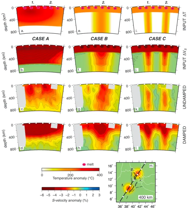
We performed a range of resolution tests to assess the quality of our retrieved tomographic models. Standard checkerboard tests are included in the Figures S9 and S10, as well as several tests for how much smearing occurs from structures above and below the transition zone into the transition zone (Figure S11). In addition, we run a set of tests for the three alternative plume hypotheses (Figure 3): (a) a large-scale plume headfilling all of the upper mantle, (b) a single plume (with assigned width of 380 km, defined as the distance where the anomaly amplitude is 20% of that in the center of the synthetic plume structure), and (c) two narrow vertical plumes (with widths of 150 km). For cases B and C a hot layer is added at the top of the input structures to mimic plume material spread in the rift zone below the plate. As a starting model for the damped plume reso-lution tests, we used the corresponding synthetic input models,filtered to mimic the effect of the surface wave resolution. Thefilter applies a variable vertical averaging (lower vertical resolution as absolute depth increases) and a variable Gaussian spatialfilter (lower spatial resolution as depth increases).
The checkerboard tests illustrate that we achieve quite good resolution for anomalies of 125 km and 250 km diameter through most of the transition zone (Figures S9 and S10). At shallow depths (around 100 km), the resolved area is confined to directly below the stations, and from about 300 km depth covers much of the region of interest shown in Figure 1. At the edges of the model, the checkers become more smeared with depth. For 125 km sized features, resolution becomes poor below about 600 km depth for most of the area Figure 2. Trade-off between S/SKS-velocity model roughness and datafit for
inversions with different degrees offlattening and smoothing (symbols) and three different degrees of damping toward the surface wave-constrained initial structure (colors). The dashed line represents our estimate of travel time residual error (see text for details). The regularization parameters for our preferred model are 4800 forflattening and 153,600 for smoothing and a damping of 35 (red star).
Figure 3. Three synthetic tests to examine the resolving power of our tomographic inversion for three previously proposed mantle upwelling structures: (a–d) case A —superplume, (e–h) case B—single plume, and (i–l) case C—multiple plume scenarios. Vertical cross sections through the input and output models are shown in Figures 3a–3l. (m) The location of the cross section is shown on a depth slice through the two-plume velocity input. Input models are defined in terms of temperature anomalies (Figures 3a, 3e, and 3i) and then multiplied by the isomorphic derivative from Figure S12 to obtain VSanomalies (Figures 3b, 3f, and 3h). In all cases, a set of
4% VSchecker anomalies below the rift is added to the plume structures above 100 km depth to mimic lateral variability due to lithospheric topography and melt
concentration. (Figures 3a–3d) Case A: superplume represented by a flat ellipsoid with a maximum excess T of 400°C at 120 km depth and a Gaussian falloff with depth leading to 0° anomalies at 660 km. (Figures 3e–3h) Case B: single larger upwelling modeled as a vertical cylinder positioned beneath Afar with maximum 200°C excess temperature that is constant with depth and Gaussian variation laterally over a 380 km width (defined as the distance to 20% of the maximum amplitude), plus a layer of 200°C excess temperature above 200 km depth. (Figures 3i–3l) Case C: two smaller upwellings represented by vertical cylinders, positioned beneath Afar and MER, again assuming a maximum 200°C T anomaly that is constant with depth, a Gaussian variation laterally over a 150 km width, and a 200°C hot layer above 200 km depth. (Figures 3c, 3g, and 3k) Recovered models using the same parameters as in the data inversion but with no damping. (Figures 3d, 3h, and 3l) Recovered models using the same parameters as in the data inversion, including damping (factor = 35). The starting model to which the inversion is damped is a version of the 3-D synthetic model down to a depth of 350 km smoothed to mimic spatial resolution of F2010. Regions with less thanfive rays per node are shaded gray. The spacing between the contours is 0.25%. The white points indicate the distance every 2°. Profiles through the center of the plumes showing the input and retrieved anomalies are shown in Figure S15. These tests illustrate that without damping most shallow structure is not recovered. Damped inversions yield a better representation of the vertical continuity of the plume structures.
(Figure S10). Larger features, with diameters of at least 250 km, are resolved over a wider region and through the transition zone, down to 700–800 km depth (Figure S9).
The plume tests in Figure 3 illustrate the importance of using a priori constraints for the shallow structure in the starting model and damping toward these structures. Without such constraints, the expected laterally widespread low-velocity structures above 200 km depth cannot be retrieved. While undamped inversions emphasize lateral variations in velocity structures, which in the case of models B and C means the plume tails, in the damped inversions the geometry of the imaged structures is much closer to that of the input struc-tures. Note that due to the decrease in thermal sensitivity of VS with depth (from about 3%/100 K at
100 km depth to<1%/100 K at 600 km depth; Figure S12) and the expectation that temperatures of adiabatic upwellings only change by a few tens of degrees over the depth of the upper mantle, we would expect plume anomalies to decrease with depth. Thus, tomographic images of upper mantle plumes are not expected to have simple cylindrical morphologies.
3.2.S Velocity Structure
Our preferred S-SKS model (with intermediate damping) is shown in Figure 4. Undamped and strongly damped models are included as Figures S3 and S4. The color scale used is the same in all panels to illus-trate how anomaly amplitudes vary with depth. The scale best illusillus-trates the transition zone anomalies and saturates at depths from 300 km upward, for which the structures have been analyzed in detail in previous studies [Bastow et al., 2005; Bastow et al., 2008; Hammond et al., 2013]. The damped models in particular emphasize that the strongest low velocities are shallow, where they are widespread. Deep structures persist at all degrees of damping and are hence required by the data. Also, the synthetic test for a large anomaly confined to the top 400 km shows limited smearing to deeper depths (Figure S11), illustrating that the transition zone anomalies are not a result of smearing.
Station terms are mostly negative below the oceanic Red Sea and generally positive beneath the African con-tinent. Some of the negative station corrections under Arabia and the Afar Depression may in effect be a compensation for lateral smearing of the low velocity from northeastern Africa in the surface wave model (compare with the undamped case in Figure S3, where these stations have positive corrections). Overall, the station correction trend reflects crustal structure [e.g., Hammond et al., 2011].
The mantle structure shows the samefirst-order features as NEAR-P15 [Civiero et al., 2015]. The shallow upper mantle, down to ~100 km, reveals a broad low-velocity layer with the strongest anomalies following the rift morphology ( 4.5%< δVS< 3.0%), similar to other previous tomographic studies for this region [e.g.,
Bastow et al., 2008; Fishwick, 2010; Hammond et al., 2013].
At larger depths, the low-velocity structure splits into several separate anomalies that persist down to at least ~650 km depth. In NEAR-P15, these deeper anomalies clearly form two clusters, each about ~400 km in diameter, beneath Afar and west of the Main Ethiopian Rift (MER; Figure S5), correlating with active vol-canism in the Afar region and volvol-canism along and off axis of the MER. In the S-SKS model, the same two clusters are also clear from about 200 to 400 km depth. In the transition zone, the Afar cluster is more strongly defined than the one below the MER, which breaks up into several smaller-scale features. Note that, in NEAR-P15, the clusters also contained additional small-scale structure in the transition zone (Figures S5 and S6).
The amplitude of the low-velocity features in the intermediately damped case decreases with depth from ~ 4% in the uppermost mantle to ~ 0.5% below the transition zone. The deepest resolution is too limited to determine how the transition zone structure relates with that below 600–700 km depth.
Complexity in the structure may be to some extent influenced by anisotropy. However, we have quite good azimuthal coverage (as shown in Figure S8), where the core of the region is traversed by rays span-ning an azimuthal range of 270–360°, which should aid in averaging out azimuthal anisotropic effects. And although we combine SH and SV data, we get images that are quite consistent with those of the P data, so if radial anisotropy exists it does not appear to map significantly into the S structures we resolve. Nonetheless, this would be an aspect that warrants future work.
Vertical cross sections through the models (Figure 5) further illustrate the vertical continuity of the two clus-ters from the shallow mantle through the transition zone, again consistent with the P wave structure.
However, different from the P velocity structure (Figures S5 and S6), the anomalies below Afar are stronger in amplitude and more continuous than the anomalies west of the MER (see profiles E-F and G-H in Figure 5).
4. Physical Interpretation
4.1. Ratio ofP and S Velocity Anomalies
Several studies have used the ratio of relative changes in shear and compressional wave velocities, defined as RS,P(=dlnVS/dlnVP= [dVS/VS]/[dVP/VP]), as diagnostic of the cause of the seismic anomalies [e.g., Karato and
Figure 4. Depth slices through our S-SKS preferred intermediate-damped tomographic model (flattening = 4800, smoothing = 153,600, damping = 35), at depths between 200 and 700 km. Regions with less thanfive rays per node are shaded gray (a version where regions with less than 10 rays per node are shaded can be found in Figure S2). The spacing between the contours is 0.5%. The black lines delineate the major border faults and magmatic zones bounding the Afar Depression, and the black over white lines show the coastlines. The triangular and square symbols in Figure 4g represent the sign and magnitude of the station static terms. Compare with Figure S5 to see thefirst-order similarities in structure between the independently inverted S/SKS and P velocity models. Compared to the undamped model (Figure S3), the shallow mantle anomalies are enhanced and more extensive. Otherwise, similar features, including the low velocities below Afar and west of the MER, appear.
Karki, 2001; Masters et al., 2000; Robertson and Woodhouse, 1996; Simmons et al., 2009]. The expected RS,Pfor
purely thermal variations spans a range from 1.3 (for low values of temperature, with a weak anelasticity effect) to 2.2 (at high temperatures, where the anelasticity effect is strong) [Cammarano et al., 2003; Goes et al., 2000]. Where water is present, it may enhance the anelastic sensitivity to temperature by lowering the melting temperature [Karato and Jung, 1998] and/or form hydrated minerals that usually have lower velo-city than average mantle minerals [e.g., Abers and Hacker, 2016; Angel et al., 2001]. The anelastic effects of fluids can increase RS,Pto up to about 2.3; hydrous minerals, if present in large enough quantities possibly
somewhat more [e.g., Goes et al., 2000; Hacker and Abers, 2012].
Figure 5. (a–i) Vertical cross sections through the S-SKS model and (j and k) comparison with a section through NEAR-P15. Regions with less than five rays per node are shaded gray. The spacing between the contours is 0.5% for the S model and 0.25% for the P model. The white circles along the top of the vertical profiles mark the distance every 2°. (Figures 5a–5d) Damped (damping = 35) and (Figures 5e and 5f) undamped (damping = 0) S-SKS models (both have flattening = 4800, smooth-ing = 153,600). The location of the cross sections (black lines) is shown in the 500 km depth slice through the damped model (Figure 5i). Cross sections A-B, C-D, E-F, and G-H have the same orientations as the profiles through the P velocity models in Figures 5j and 5k and Figure S6. The undamped models (Figures 5e–5h) emphasize the stronger amplitude of the low-velocity cluster below Afar compared to that beneath MER; the damped models (Figures 5a–5d) show that the low-velocity anomalies extend from the surface to at least the bottom of the transition zone. The features in S model are similar to those seen in the P model (Figures 5j and 5k).
For most plausible large-scale com-positions (i.e., more or less melt-depleted forms of peridotite or alternative chondritic composi-tions), the effect of composition on VPand VSabove the transition
zone is small compared to that of temperature [Afonso et al., 2010; Cammarano et al., 2003; Goes et al., 2000; Worthington et al., 2013]. In the transition zone, the sensitivity of velocity to changes in composition is complicated by the different depths, Clapeyron slopes, and widths of the phase transitions expected for different bulk compositions [Cammarano et al., 2003; Xu et al., 2008]. Overall, for most upper mantle composi-tions and depths, the sensitivity of RS,Pto temperature and composi-tion is likely not different enough to distinguish the two factors. The largest effects on RS,P are
expected from partial melt [e.g., Faul et al., 2004; Hammond and Kendall, 2016; Hammond and Humphreys, 2000; Schmeling, 1985] with values that can range from around 1.6 for ellipsoidal melt inclusions, to 2.2 forfilms in a geo-metry taken from natural samples [Hammond and Humphreys, 2000], to up to 4.0 for alignedfilm and layer geometries [Takei, 2002], which would also lead to strong anisotropy.
Several studies use the ratio of P and S wave relative arrival-time residualsδS,P, i.e., using the data rather than
the tomographically imaged anomalies [e.g., Bastow et al., 2005; Gao et al., 2004; Rocha et al., 2011].δS,Pshould
be proportional to the ratio of absolute dVSand dVPalong the chosen station-event pairs. Thus, the slopeδS,P
equals (VP/VS) RS,Por about√3 times RS,P. Bastow et al. [2005] perform aδS,Panalysis below the Main Ethiopian Rift andfind a gradient between ~5 and ~10, which they attribute to significant fractions of shallow melt ponding beneath the rift, consistent with other geochemical and geophysical results [e.g., Bastow et al., 2005; Ebinger and Casey, 2001; Gao et al., 1997; Hammond et al., 2014; Kendall et al., 2005; Rooney et al., 2007]. Other studies have usedδS,Pto argue for chemical heterogeneity. For example, Gao et al. [2004]
con-clude aδS,Pof ~2.9 for fast anomalies below the Colorado Plateau is on the high side to invoke temperature perturbations. Similarly, Rocha et al. [2011]find δS,P> 2.9 below the São Francisco Craton and interpret it as
due to compositional effects. However, from our preceding discussion of the expected range of RS,Pvalues
including the effect of anelasticity,δS,Pup to 3.6–3.8 correspond to RS,Pwhich fall within the thermal range.
To get further insight into the possible physical causes of the seismic anomalies we imaged below the north-ern East African Rift, we perform a comparison of the P and S-SKS wave relative arrival-time residuals for com-mon events (Figure 6). Prior to the analysis, we remove all residuals downweighted by the Huber iterations. A straight linefit through our measurements (least squares, accounting for the estimated picking errors) yields aδS,Pof 3.69 ± 0.01, which corresponds to an RS,Pof ~2.1. This value is toward the higher end of estimates of
purely thermal RS,Pbetween ~1.3 and 2.2 [Cammarano et al., 2003; Goes et al., 2000], and is as expected, given
Figure 6. P wave [from Civiero et al., 2015] versus S wave (this study) relative arrival-time residuals for all common earthquakes. The solid red line is a least squaresfit including picking errors for all data (blue and white circles) and has a gradient,δS,P, of 3.69 ± 0.01 for all data corresponding to a ratio RS, P= lnVS/dlnVPof ~2.1, consistent with a dominantly thermal origin of the
anomalies. The dashed red line is a least squaresfit including only data close to the MER (white circles) and has a gradient of 5.60 ± 0.03 (RS,P= ~3.2),
previously interpreted as implying the presence of melt in a region around the MER [Bastow et al., 2005].
the likely elevated mantle temperatures (and thus expected higher anelasticity effect) below the region indi-cated by previous work [Armitage et al., 2015; Ferguson et al., 2013; Rooney et al., 2012].
This result seems contradictory to the previousδS,P, between ~5 and ~10, for stations within the MER [Bastow
et al., 2005]. However, when we calculate theδS,Ponly for the subset of stations centered around MER (i.e.,
more or less corresponding to the area covered by the Ethiopia Afar Geoscientific Lithospheric Experiment that Bastow et al. [2005] analyzed), wefind a higher slope of 5.60 ± 0.03 corresponding to an RS,P~3.2. This
indicates that what Bastow et al. [2005] interpreted as the signature of melt is likely local and shallow. Our new travel time data set covers a significantly longer time span and a larger region of the rift, and thus, the effects of local shallow melt signatures are mixed in with deeper mantle thermal signatures.
We also computed RS,Pvalues after the tomographic inversion. These ratios are strongly scattered, ranging
from about 0 to 4 (Figure S13), as they are affected by any differences in spatial resolution of the two models. For this reason, care must be taken interpreting the RS,Pdistribution. Broadly, the RS,Pdistribution is peaked in
the thermal range (median 1.7 for damping = 35). The RS,Pin the damped models is more strongly peaked in
the thermal range, as it is conditioned by our thermally scaled starting model for P. This does however con-firm that a thermal interpretation is compatible with the data. Also, as expected for thermal mechanisms (but also from melt or hydration), the peak in RS,Pshifts to higher values in low-velocity regions (median 1.9 for
damping = 35; Figure S14). This trend is seen in both damped and undamped models.
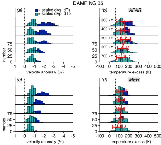
Figure 7. Histograms showing the range of velocity anomalies, after scaling for resolution, and the corresponding tem-perature anomalies from the NEAR-P15 P and NEAR-S16 S/SKS wave models (with a degree of damping of 35), at depths ranging from 300 to 700 km. The two regions considered are outlined by the boxes in Figure S5 for P and Figure S7 for S: (a and b) Afar Depression and (c and d) west of the MER. Figures 7a and 7c show in light green the P wave velocity anomalies scaled according to the resolution as a function of depth based on the P wave synthetic test in Civiero et al. [2015], and in dark blue the S-SKS wave velocity anomalies scaled according to the resolution as a function of depth based on the reso-lution test in Figures 3 and S15. The red dashed bars in Figures 7b and 7d illustrate the mean and standard deviation of the temperature excess for P velocity anomalies estimated in each region; the red solid bars denote the mean and standard deviation of the temperature excess for S velocity anomalies. These values show that temperatures inferred from dVPand dVSare in a similar thermal range of 100–200°C from 300 to 700 km depth.
4.2. Temperature Estimates
As, tofirst order, the anomalies appear to be thermal in nature, we convert the low-velocity anomalies in the two main clusters (see boxes in Figure S7) to temperature anomalies, using the same method as in Civiero et al. [2015]. To account for the fact that the tomography underresolves anomaly amplitudes and the recov-ered amplitudes depend on regularization, wefirst scale (Figure 7a) the S velocities according to the ampli-tude resolution with depth estimated from an idealized plume model (Figures 3 and S15). The effect and uncertainties of the amplitude resolution are discussed in detail in Civiero et al. [2015], where the results from differently damped inversions were in a similar range. Next, the scaled dVSanomalies are converted to dT
using a smooth dVS/dT derivative for a pyrolitic composition along a 1300°C adiabat (taken from Styles
et al. [2011]; Figure S12). Uncertainties in this conversion to temperature anomalies are a few tens of degrees including consideration of uncertainties in the reference profile, and would largely work in the same direction for the conversion from P and S velocity anomalies, as both depend on shear modulus and density. Figure 7b shows that the inferred estimates of excess temperatures for both wave speeds agree well within their uncer-tainties and scatter and fall between 100 and 200°C.
Note that although the temperature estimates from dVPand dVSfor both the Afar and MER clusters agree, the
significant uncertainties and scatter would allow for some influence of other mechanisms. dTSestimates tend
to be slightly higher than dTPabove 500 km depth, while at larger depths dTStends to be somewhat lower
than dTP. The latter is probably due to the stronger decrease of the resolution with depth of VSthan VP. The former may be a hint of a signature of deep melts. Thompson et al. [2015] used receiver functions to image a distinct low-velocity zone above the transition zone beneath Afar. They interpreted this to be a melt layer caused by the release of volatiles from an upwelling below Afar. Rooney et al. [2012] also proposed a contribution of deep CO2-assisted melting to the very slow velocities below Afar. Our tomographic model
does not have the resolution to distinguish such local features [Civiero et al., 2015] but does leave room for such an interpretation.
Our temperature estimates are consistent with those inferred from geochemistry and petrology [Ferguson et al., 2013; Rooney et al., 2012], from seismic studies of the shallow mantle [Armitage et al., 2015; Rychert Figure 8. Comparison of global tomographic model SGLOBE-RANI [Chang et al., 2015] and NEAR-S16. (a) Vertical section through SGLOBE-RANI. The white dots are spaced 10°. (b) The top 800 km, our model NEAR-S16, structure below 800 km (marked by a white line) SGLOBE-RANI. NEAR-S16 is shaded gray, where there are less thanfive rays per node. Note the consistency between the two models, with NEAR-S16 resolving more small-scale structure inside the large low-velocity region in SGLOBE-RANI. (c) Map shows the location of the vertical cross section on a horizontal slice at 500 km depth through model SGLOBE-RANI.
et al., 2012] and transition zone [Thompson et al., 2015], and from estimates of melt production [Armitage et al., 2015]. The estimates are lower than inferred below some other hot spots, e.g., Hawaii, North Atlantic, and Deccan [Armitage et al., 2010; Watson and McKenzie, 1991]. They are also somewhat lower than those from Mulibo and Nyblade [2013], who in a recent tomographic study conclude that a thermal perturbation of ~150–300 K reconciles P and S wave velocities beneath Tanzania and northwestern Zambia. The tempera-ture estimates below the northern EAR are consistent with the interpretation that the low velocities through the transition zone are due to warm thermal upwellings.
5. Conclusions
In this study, we combine S and SKS wave relative travel times to achieve a high-resolution tomographic shear wave model, NEAR-S16, that extends throughout the whole upper mantle below of the northern East Africa. This S model complements a recent P travel time model, NEAR-P15, for the same region [Civiero et al., 2015]. The patterns of P and S wave velocities strongly resemble each other in terms of geometry and scale. The tomographic images reveal widespread low velocities in the upper 200 km of the mantle below the region. Below this depth, two clusters of low velocities emerge, situated below Afar and west of the MER. These extend through the transition zone. Both the P and S low-velocity anomalies yield excess temperature esti-mates in the range of 100–200°C in these two clusters. These results give us more confidence in interpreting the structure imaged in both P and S-SKS wave models below the northern East African Rift as being mainly the signature of multiple small-scale upper mantle thermal upwellings.
A comparison of our imaged structure with that of previous global tomographic studies reveals the consis-tency of our structures with these large-scale models, as shown in Figure 8 for the global anisotropic S velo-city model SGLOBE-RANI [Chang et al., 2015]. As more data have been added to the global models, the complexity of the low-velocity structure below the East African Rift has increased, e.g., compare S20RTS [Ritsema and van Heijst, 2000], which imaged a single large-scale feature that appeared to be continuous from the lower mantle below southern Africa to the upper mantle from Kenya/Tanzania to Afar, with S40RTS [Ritsema et al., 2011] and SGLOBE-RANI [Chang et al., 2015], whichfind two low-velocity anomalies in the upper mantle below Kenya/Tanzania and Afar, as well as variability within the lower mantle, low-velocity anomalies (Figure 8). The comparison between our travel time model and the global model SRANI clearly shows that what appeared like one large-scale feature below Afar in several previous studies [e.g., Hansen et al., 2012] has in fact internal small-scale structure, as was previously suggested based on surface wave tomography by Debayle et al. [2001]. Models S40RTS and SGLOBE-RANI even hint at a low-velocity anomaly at the base of the transition zone directly below the strong low velocities we image. As discussed fully in Civiero et al. [2015], this might be a ponding of warm material that forms the source of the small-scale upwel-lings we infer, a feature that is seen in analogue and numerical models of plume transition-zone interaction [e.g., Kumagai et al., 2007; Tosi and Yuen, 2011]. Evaluation of the global models along different cross sections indicates that this velocity region at the base of the transition zone may connect with one of the low-velocity features that appear to rise off the Large Low-Shear-Velocity Provinces below Africa. Further work to improve resolution of lower mantle structure below the rift system with more stations and/or by making use of a larger part of the waveforms will be necessary to identify the lower mantle source of the small-scale shallow mantle upwellings.
References
Abers, G. A., and B. R. Hacker (2016), A MATLAB toolbox and Excel workbook for calculating the densities, seismic wave speeds, and major element composition of minerals and rocks at pressure and temperature, Geochem. Geophys. Geosyst., 17, 616–624, doi:10.1002/ 2015GC006171.
Afonso, J. C., G. Ranalli, M. Fernàndez, W. L. Griffin, S. Y. O’Reilly, and U. Faul (2010), On the Vp/Vs–Mg# correlation in mantle peridotites: Implications for the identification of thermal and compositional anomalies in the upper mantle, Earth Planet. Sci. Lett., 289(3), 606–618. Angel, R. J., D. J. Frost, N. L. Ross, and R. Hemley (2001), Stabilities and equations of state of dense hydrous magnesium silicates, Phys. Earth
Planet. Int., 127(1), 181–196.
Armitage, J. J., J. S. Collier, and T. A. Minshull (2010), The importance of rift history for volcanic margin formation, Nature, 465(7300), 913–917. Armitage, J. J., D. J. Ferguson, S. Goes, J. O. S. Hammond, E. Calais, C. A. Rychert, and N. Harmon (2015), Upper mantle temperature and the
onset of extension and break-up in Afar, Africa, Earth Planet. Sci. Lett., 418, 78–90.
Bastow, I. D., G. W. Stuart, J. M. Kendall, and C. J. Ebinger (2005), Upper-mantle seismic structure in a region of incipient continental breakup: Northern Ethiopian rift, Geophys. J. Int., 162(2), 479–493.
Bastow, I. D., A. A. Nyblade, G. W. Stuart, T. O. Rooney, and M. H. Benoit (2008), Upper mantle seismic structure beneath the Ethiopian hot spot: Rifting at the edge of the African low-velocity anomaly, Geochem. Geophys. Geosyst., 9, Q12022, doi:10.1029/2008GC002107.
Acknowledgments
We would like to thank the many peo-ple involved in the collection of data used in this study. Data specifically pro-vided for this study include those recorded by instruments in Yemen, Ethiopia, and Eritrea provided by SEIS-UK. The facilities of SEIS-UK are sup-ported by the Natural Environment Research Council under agreement R8/H10/64. These data will be available at the IRIS-DMC in 2016 (http://ds.iris. edu/ds/nodes/dmc/). The data from the Djibouti deployment were provided by RESIF (http://www.resif.fr; ANR-11-EQPX-0040). The instruments deployed in Uganda-Congo were provided by the Geophysical Instrument Pool Potsdam, and data are archived at the GEOFON data center (http://geofon.gfz-potsdam. de). The permanent instruments in Ethiopia are run by the Institute of Space Science, Geophysics and Astronomy, Addis Ababa University (contact for data: atalay.ayele@aau.edu. et) andfinancial support for most of the Ethiopian permanent seismic stations comes from the International Science Program of Uppsala University (Sweden). Other data were downloaded from the IRIS and GEOFON data centers. Funding for data collection was pro-vided by NERC grants NE/E007414/1 and NE/J012297/1 and BHP-Billiton. We thank Ana Fereira for providing the model SGLOBE-RANI and Ian Bastow and John Armitage for their discussions. C.C. was supported by a Janet Watson Fellowship from the Department of Earth Science and Engineering at Imperial College, J.H. by NERC Fellowship NE/I020342/1, and D.K. by NERC grant NE/L013932/1.
Benoit, M. H., A. A. Nyblade, and J. C. VanDecar (2006), Upper mantle P-wave speed variations beneath Ethiopia and the origin of the Afar hotspot, Geology, 34(5), 329–332.
Burke, K. (1996), The African plate, S. Afr. J. Geol., 99, 339–410.
Cammarano, F., S. Goes, P. Vacher, and D. Giardini (2003), Inferring upper-mantle temperatures from seismic velocities, Phys. Earth Planet. Inter., 138(3–4), 197–222.
Chang, S.-J., and S. Van der Lee (2011), Mantle plumes and associatedflow beneath Arabia and East Africa, Earth Planet. Sci. Lett., 302(3–4), 448–454.
Chang, S.-J., A. M. G. Ferreira, J. Ritsema, H. J. van Heijst, and J. H. Woodhouse (2015), Joint inversion for global isotropic and radially anisotropic mantle structure including crustal thickness perturbations, J. Geophys. Res. Solid Earth, 120, 4278–4300, doi:10.1002/ 2014JB011824.
Civiero, C., J. O. S. Hammond, S. Goes, S. Fishwick, A. Ahmed, A. Ayele, C. Doubre, B. Goitom, D. Keir, and J. Kendall (2015), Multiple mantle upwellings in the transition zone beneath the northern East-African Rift system from relative P-wave travel-time tomography, Geochem. Geophys. Geosyst., 16, 2949–2968, doi:10.1002/2015GC005948.
Daradich, A., J. X. Mitrovica, R. N. Pysklywec, S. D. Willett, and A. M. Forte (2003), Mantleflow, dynamic topography, and rift-flank uplift of Arabia, Geology, 31(10), 901–904.
Debayle, E., J.-J. Lévêque, and M. Cara (2001), Seismic evidence for a deeply rooted low-velocity anomaly in the upper mantle beneath the northeastern Afro/Arabian continent, Earth Planet. Sci. Lett., 193(3–4), 423–436.
Ebinger, C. J., and M. Casey (2001), Continental breakup in magmatic provinces: An Ethiopian example, Geology, 29(6), 527–530. Ebinger, C. J., and N. H. Sleep (1998), Cenozoic magmatism throughout east Africa resulting from impact of a single plume, Nature, 395(6704),
788–791.
Faul, U. H., J. D. Fitz Gerald, and I. Jackson (2004), Shear wave attenuation and dispersion in melt-bearing olivine polycrystals: 2. Microstructural interpretation and seismological implications, J. Geophys. Res., 109, B06202, doi:10.1029/2003JB002407.
Ferguson, D. J., J. Maclennan, I. D. Bastow, D. M. Pyle, S. M. Jones, D. Keir, J. D. Blundy, T. Plank, and G. Yirgu (2013), Melting during late-stage rifting in Afar is hot and deep, Nature, 499, 70–73.
Fishwick, S. (2010), Surface wave tomography: Imaging of the lithosphere–asthenosphere boundary beneath central and southern Africa?, Lithos, 120(1–2), 63–73.
Furman, T., J. G. Bryce, J. Karson, and A. Iotti (2004), East African Rift System (EARS) plume structure: Insights from Quaternary mafic lavas of Turkana, Kenya, J. Petrol., 45(5), 1069–1088.
Furman, T., J. Bryce, T. Rooney, B. Hanan, G. Yirgu, and D. Ayalew (2006), Heads and tails: 30 million years of the Afar plume, Geol. Soc. London, Spec. Publ., 259(1), 95–119.
Gao, S. S., K. H. Liu, and M. G. Abdelsalam (2010), Seismic anisotropy beneath the Afar Depression and adjacent areas: Implications for mantle flow, J. Geophys. Res., 115, B12330, doi:10.1029/2009JB007141.
Gao, S., P. M. Davis, H. Liu, P. D. Slack, A. W. Rigor, Y. A. Zorin, V. V. Mordvinova, V. M. Kozhevnikov, and N. A. Logatchev (1997), SKS splitting beneath continental rift zones, J. Geophys. Res., 102(B10), 22,781–22,797, doi:10.1029/97JB01858.
Gao, W., S. P. Grand, W. S. Baldridge, D. Wilson, M. West, J. F. Ni, and R. Aster (2004), Upper mantle convection beneath the central Rio Grande rift imaged by P and S wave tomography, J. Geophys. Res., 109, B03305, doi:10.1029/2003JB002743.
George, R., N. Rogers, and S. Kelley (1998), Earliest magmatism in Ethiopia: Evidence for two mantle plumes in oneflood basalt province, Geology, 26(10), 923–926.
Goes, S., R. Govers, and P. Vacher (2000), Shallow mantle temperatures under Europe from P and S wave tomography, J. Geophys. Res., 105(B5), 11,153–11,169, doi:10.1029/1999JB900300.
Hacker, B. R., and G. A. Abers (2012), Subduction Factory 5: Unusually low Poisson’s ratios in subduction zones from elastic anisotropy of peridotite, J. Geophys. Res., 117, B06308, doi:10.1029/2012JB009187.
Hammond, J. O. S., and J. M. Kendall (2016), Constraints on melt distribution from seismology: A case study in Ethiopia, in Magmatic Rifting and Active Volcanism, edited by T. J. Wright et al., Geol. Soc. London, Spec. Publ., 420, 127–147.
Hammond, J. O. S., J. M. Kendall, G. W. Stuart, D. Keir, C. Ebinger, A. Ayele, and M. Belachew (2011), The nature of the crust beneath the Afar triple junction: Evidence from receiver functions, Geochem. Geophys. Geosyst., 12, Q12004, doi:10.1029/2011GC003738.
Hammond, J. O. S., et al. (2013), Mantle upwelling and initiation of rift segmentation beneath the Afar Depression, Geology, 41(6), 635–638.
Hammond, J. O. S., J. M. Kendall, J. Wookey, G. W. Stuart, D. Keir, and A. Ayele (2014), Differentiatingflow, melt or fossil anisotropy beneath Ethiopia, Geochem. Geophys. Geosyst., 15, 1878–1894, doi:10.1002/2013GC005185.
Hammond, W. C., and E. D. Humphreys (2000), Upper mantle seismic wave attenuation—Effects of realistic partial melt geometries, J. Geophys. Res., 105(B5), 10,987–10,999, doi:10.1029/2000JB900042.
Hansen, S. E., A. A. Nyblade, and M. H. Benoit (2012), Mantle structure beneath Africa and Arabia from adaptively parameterized P-wave tomography: Implications for the origin of Cenozoic Afro-Arabian tectonism, Earth Planet. Sci. Lett., 319–320, 23–34.
Huber, P. J. (1981), Robust Statistics, John Wiley, New York.
Karato, S.-I., and B. B. Karki (2001), Origin of lateral variation of seismic wave velocities and density in the deep mantle, J. Geophys. Res., 106(R10), 21,771–21,783, doi:10.1029/2001JB000214.
Karato, S.-I., and H. Jung (1998), Water, partial melting and the origin of the seismic low velocity and high attenuation zone in the upper mantle, Earth Planet. Sci. Lett., 157(3), 193–207.
Kendall, J. M., G. W. Stuart, C. J. Ebinger, I. D. Bastow, and D. Keir (2005), Magma-assisted rifting in Ethiopia, Nature, 433(7022), 146–148.
Koulakov, I. Y. (2007), Structure of the Afar and Tanzania plumes based on the regional tomography using ISC data, Dokl. Earth Sci., 417(1), 1287–1292.
Kumagai, I., A. Davaille, and K. Kurita (2007), On the fate of thermally buoyant mantle plumes at density interfaces, Earth Planet. Sci. Lett., 254, 180–193.
Lin, S.-C., B.-Y. Kuo, L.-Y. Chiao, and P. E. van Keken (2005), Thermal plume models and melt generation in East Africa: A dynamic modeling approach, Earth Planet. Sci. Lett., 237(1-2), 175–192.
Masters, G., G. Laske, H. Bolton, and A. Dziewonski (2000), The relative behavior of shear velocity, bulk sound speed, and compressional velocity in the mantle: Implications for chemical and thermal structure, in Earth’s Deep Interior: Mineral Physics and Tomography From the Atomic to the Global Scale, edited by S.-I. Karato et al., pp. 63–87, AGU, Washington, D. C.
Meshesha, D., and R. Shinjo (2008), Rethinking geochemical feature of the Afar and Kenya mantle plumes and geodynamic implications, J. Geophys. Res., 113, B09209, doi:10.1029/2007JB005549.
Montagner, J.-P., B. Marty, E. Stutzmann, D. Sicilia, M. Cara, R. Pik, J.-J. Lévêque, G. Roult, E. Beucler, and E. Debayle (2007), Mantle upwellings and convective instabilities revealed by seismic tomography and helium isotope geochemistry beneath eastern Africa, Geophys. Res. Lett., 34, L21303, doi:10.1029/2007GL031098.
Montelli, R., G. Nolet, G. Masters, F. A. Dahlen, and S. H. Hung (2004a), Global P and PP traveltime tomography: Rays versus waves, Geophys. J. Int., 158(2), 637–654.
Montelli, R., G. Nolet, F. A. Dahlen, G. Masters, E. R. Engdahl, and S.-H. Hung (2004b), Finite-frequency tomography reveals a variety of plumes in the mantle, Science, 303(5656), 338–343.
Mulibo, G. D., and A. A. Nyblade (2013), The P and S wave velocity structure of the mantle beneath eastern Africa and the African superplume anomaly, Geochem. Geophys. Geosyst., 14, 2696–2715, doi:10.1002/ggge.20150.
Peter, D., L. Boschi, and J. H. Woodhouse (2009), Tomographic resolution of ray andfinite-frequency methods: A membrane-wave investi-gation, Geophys. J. Int., 177(2), 624–638.
Pik, R., B. Marty, and D. R. Hilton (2006), How many mantle plumes in Africa? The geochemical point of view, Chem. Geol., 226(3–4), 100–114. Reed, C. A., S. S. Gao, K. H. Liu, and Y. Yu (2016), The mantle transition zone beneath the Afar Depression and adjacent regions: Implications
for mantle plumes and hydration, Geophys. J. Int., 205, 1756–1766.
Ritsema, J., and H. J. van Heijst (2000), Seismic imaging of structural heterogeneity in Earth’s mantle: Evidence for large-scale mantle flow, Sci. Prog., 83(3), 243–259.
Ritsema, J., A. A. Nyblade, T. J. Owens, C. A. Langston, and J. C. VanDecar (1998), Upper mantle seismic velocity structure beneath Tanzania, East Africa: Implications for the stability of cratonic lithosphere, J. Geophys. Res., 103, 21,201–221,213, doi:10.1029/98JB01274. Ritsema, J., H. J. V. Heijst, and J. H. Woodhouse (1999), Complex shear wave velocity structure imaged beneath Africa and Iceland, Science,
286(5446), 1925–1928.
Ritsema, J., A. Deuss, H. J. van Heijst, and J. H. Woodhouse (2011), S40RTS: A degree-40 shear-velocity model for the mantle from new Rayleigh wave dispersion, teleseismic traveltime and normal-mode splitting function measurements, Geophys. J. Int., 184(3), 1223–1236. Robertson, G. S., and J. H. Woodhouse (1996), Ratio of relative S to P velocity heterogeneity in the lower mantle, J. Geophys. Res., 101(B9),
20,041–20,052, doi:10.1029/96JB01905.
Rocha, M. P., M. Schimmel, and M. Assumpção (2011), Upper-mantle seismic structure beneath SE and central Brazil from P- and S-wave regional traveltime tomography, Geophys. J. Int., 184(1), 268–286.
Rogers, N. W., R. Macdonald, J. G. Fitton, R. George, M. Smith, and B. Barreiro (2000), Two mantle plumes beneath the East African Rift system: Sr, Nd and Pb isotope evidence from Kenya Rift basalts, Earth Planet. Sci. Lett., 176, 387–400.
Rooney, T. O., C. Herzberg, and I. D. Bastow (2012), Elevated mantle temperature beneath East Africa, Geology, 40(1), 27–30.
Rooney, T., T. Furman, I. Bastow, D. Ayalew, and G. Yirgu (2007), Lithospheric modification during crustal extension in the Main Ethiopian Rift, J. Geophys. Res., 112, B10201, doi:10.1029/2006JB004916.
Rychert, C. A., J. O. S. Hammond, N. Harmon, J. Michael Kendall, D. Keir, C. Ebinger, I. D. Bastow, A. Ayele, M. Belachew, and G. Stuart (2012), Volcanism in the Afar Rift sustained by decompression melting with minimal plume influence, Nat. Geosci., 5(6), 406–409.
Schimmel, M., M. Assumpçao, and J. C. VanDecar (2003), Seismic velocity anomalies beneath SE Brazil from P and S wave travel time inversions, J. Geophys. Res., 108(B4), 2191, doi:10.1029/2001JB000187.
Schmeling, H. (1985), Numerical models on the influence of partial melt on elastic, anelastic and electric properties of rocks. Part I: Elasticity and anelasticity, Phys. Earth Planet. Int., 41(1), 34–57.
Simmons, N. A., A. M. Forte, and S. P. Grand (2009), Joint seismic, geodynamic and mineral physical constraints on three-dimensional mantle heterogeneity: Implications for the relative importance of thermal versus compositional heterogeneity, Geophys. J. Int., 177(3), 1284–1304. Styles, E., S. Goes, P. E. van Keken, J. Ritsema, and H. Smith (2011), Synthetic images of dynamically predicted plumes and comparison with a
global tomographic model, Earth Planet. Sci. Lett., 311(3–4), 351–363.
Takei, Y. (2002), Effect of pore geometry on Vp/Vs: From equilibrium geometry to crack, J. Geophys. Res., 107(B2), 2043, doi:10.1029/ 2001JB000522.
Thompson, D. A., J. O. S. Hammond, J. M. Kendall, G. W. Stuart, G. R. Helffrich, D. Keir, A. Ayele, and B. Goitom (2015), Hydrous upwelling across the mantle transition zone beneath the Afar Triple Junction, Geochem. Geophys. Geosyst., 16, 834–846, doi:10.1002/2014GC005648. Tilmann, F. J., H. M. Benz, K. F. Priestley, and P. G. Okubo (2001), P-wave velocity structure of the uppermost mantle beneath Hawaii from
traveltime tomography, Geophys. J. Int., 146(3), 594–606.
Tosi, N., and D. A. Yuen (2011), Bent-shaped plumes and horizontal channelflow beneath the 660 km discontinuity, Earth Planet. Sci. Lett., 12, 348–359.
VanDecar, J. C., and R. S. Crosson (1990), Determination of teleseismic relative phase arrival times using multi-channel cross-correlation and least squares, Bull. Seismol. Soc. Am., 80(1), 150–169.
VanDecar, J. C., D. E. James, and M. Assumpcao (1995), Seismic evidence for a fossil mantle plume beneath South America and implications for plate driving forces, Nature, 378(6552), 25–31.
Watson, S., and D. McKenzie (1991), Melt generation by plumes: A study of Hawiian volcanism, J. Petrol., 32, 501–537.
Wolfe, C. J., I. T. Bjarnason, J. C. VanDecar, and S. C. Solomon (1997), Seismic structure of the Iceland mantle plume, Nature, 385, 245–247. Wolfe, C. J., S. C. Solomon, G. Laske, J. A. Collins, R. S. Detrick, J. A. Orcutt, D. Bercovici, and E. H. Hauri (2009), Mantle shear-wave velocity
structure beneath the Hawaiian hot spot, Science, 326(5958), 1388–1390.
Worthington, J. R., B. R. Hacker, and G. Zandt (2013), Distinguishing eclogite from peridotite: EBSD-based calculations of seismic velocities, Geophys. J. Int., 193, 489–505.
Xu, W., C. Lithgow-Bertelloni, L. Stixrude, and J. Ritsema (2008), The effect of bulk composition and temperature on mantle seismic structure, Earth Planet. Sci. Lett., 275(1-2), 70–79.