Lire la seconde partie de la thèse

Lire

la seconde partie

de la thèse

6.4

Aide à la sélection des évènements de

cali-bration

L’article suivant, soumis à « Hydological Sciences Journal », reprend les consi-dérations du § 6.2 et étudie des bassins des contreforts pyrénéens et de l’Aude.

6.4.1

Article : “Characterization of catchment behaviour and

rainfall selection for flash flood dedicated hydrologic model

re-gionalization: catchments of the eastern Pyrenees”

Garambois P. A. 1,2, Larnier K. 1,2, Roux H. 1,2, Labat D. 1,3, Dartus D. 1,2

1

Université de Toulouse, INPT, UPS, IMFT (Institut de Mécanique des Fluides de Toulouse), Allée Camille Soula, 31400 Toulouse, France

2

CNRS, IMFT, 31400 Toulouse, France 3

Géosciences Environnement Toulouse-Université de Toulouse-CNRS-IRD-OMP 31400 Toulouse

* Address correspondance to Pierre-André Garambois, IMFT, allée du Pr. Camille Soula, 31400 Toulouse, France; pgarambo@imft.fr

Abstract

Flash floods prediction accuracy depends strongly on rainfall quality. Hydrometeorological radar has led to several breakthroughs but measurements still rely on raingauge network to reach correct quantitative precipi-tation estimation (QPE). The underlying question is: has the raingauge network seen the part of rainfall ex-plaining hydrological response? A methodology based on global sensitivity analysis is proposed to analyse flash storm-flood events for regionalisation with a mechanistic model. Medium catchment behaviours are identified with respect to rainfall to runoff conservation. Calibration framework and quantification of bed-rock losses for bedbed-rock types are interesting basis for flash flood prediction at ungauged locations. A huge database of 43 flood events on 11 catchments has been studied. For each event a similarity approach allows discriminating rainfall products with questioning QPE. The resulting Nash efficiencies are respectively around 0.9 in calibration and 0.7 in validation for flash flood simulation for 250 km² catchments with select-ed QPE.

Key words Flash floods, QPE, global sensitivity analysis, hydrologic model calibration,

1. INTRODUCTION: PROBLEM FRAMEWORK

Hydrometeorological forecasters are sometimes facing hard decisions in a short or very short time lapse, with considerable consequences, to warn civil security organisms early enough. Indeed, in the case of flash floods generally triggered by intense and localized storms, water depth in the drainage network can reach peaks in a few minutes or a few hours [Georgakakos, 1992]. The timescale depends on the size of the catchment considered and the definition of “flash flood”, for example in the UK flash floods are floods which response time is less than 3 hours for catchment areas of 5 to 10 km², whereas in the US response time superior to 6 hours for 400 km² catchments can be called flash floods [Georgakakos and Hudlow, 1984]. Flash floods are very variable and non linear phenomenon in time and space as their generating storm. Monitoring flash floods remains a hard exercise [Borga et al., 2008] since conventional measurement networks of rain and river discharges are not able to sample effectively [Creutin

and Borga, 2003] because of scales problems. That is why hydrological forecasts are more and

more focused on detection techniques like radar [Krajewski and Smith, 2002]; high resolution hydrometeorological prediction model [Seity et al., 2011; Vincendon et al., 2011; Vincendon et

al., 2010], the knowledge of climatic antecedents of a catchment or region, state variable

initialization for event model [Roux et al., 2011; Tramblay et al., 2011b], the accountancy of uncertainty recognized as important in hydrological modelling due to model structure itself and hypothesis for error formulation.

During the last decade, numerous calls for modelling tools improvement have been heard, for example in the EU, in the US or in Australia [Handmer, 2001; Penning-Rowsell et al., 2000]. Scientific breakthroughs have been made in the field of observation capacity and modelling. For example the long-term observatory OHMCV15, covers an area of about 160*200 km² in the Cévennes-Vivarais region (France) and various numerical models have been tested in this region with the aim of deriving efficient flash flood prediction tools [Manus et al., 2009]. [Bachoc et al., 2011] describe precisely the actual operational requirements for the French hydrological network. These warning systems depend on real time information on rainfall fields, on the knowledge of flash flood hydrology, on the models that follow and their applicability. As highlighted by [Looper and Vieux, 2011], flood prediction accuracy is linked to the quality of measurements and rainfall predictions. Model robustness and uncertainty knowledge is increased by the availability and anteriority of hydrometeorological chronics, and by their space time resolution in several cases.

Precipitation estimation can be considered as one of the most important input required for hydrological forecasting and reanalysis, given that rainfall distribution and amount determines surface hydrological process and so catchment response dynamics. An adequate characterization of rainfall inputs is fundamental to success in rainfall-runoff (RR) modelling: no model, however well founded in physical theory or empirically justified by past performance, can produce accurate runoff predictions forced by inaccurate rainfall data (e.g. [Beven, 2002]). Moreover rainfall measurement errors need to be characterized [Ciach and Krajewski, 1999;

Ciach et al., 2007; Delrieu et al., 2012; Kirstetter et al., 2010], as their impact on data

assimilation in numerical weather prediction models [Caumont et al., 2006], or on predicted flow [Bardossy and Das, 2008; Kavetski et al., 2006; Moulin et al., 2009; Sun et al., 2000]. Especially when accentuated by orography, the complex physical process governing rainfall effects makes them highly variable in time and space [Krajewski et al., 2003]. [Singh, 1997] provides detailed hydrological literature on the effect of spatial and temporal variability in hydrological factors on the stream hydrograph. [Wilson et al., 1979] show that the spatial distribution and the accuracy of the precipitation input have a marked influence on the outflow hydrograph shape and timing. [Sun et al., 2002] demonstrated that errors in storm-runoff estimation are directly related to spatial data distribution and the representation of spatial

15

conditions across the catchment.

According to [Moulin et al., 2009], the general issue of the impact of rainfall inputs on RR simulation accuracy encompasses at least two main questions:

 The level of spatial and temporal discretisation needed to accurately represent the RR process dynamics through hydrological modelling.

 The assessment of the intrinsic quality of the mean areal precipitation (MAP) estimated over the whole catchment under consideration.

The first question that might depend on the resonance between rainfall field and catchment properties is not discussed in the present paper but the modelling choices will be justified. Moreover we use a distributed model which mesh is much refined than any of those available for rainfall field description. The answer to the second question depends on the measurement techniques, the type of rainfall, meteorological configuration and the study zone singularities. Weather radar coverage has drastically increased over the last two decades allowing high spatial and temporal measurements of rainfall. Thanks to radar measurements and raingauge network, important progress in quantitative precipitation estimation (QPE) have been made, as the abundance of literature on the topic can attest [Gourley and Vieux, 2006; Hazenberg et al., 2011; Krajewski and Smith, 2002; Meischner, 2004]. However QPE presents some difficulties due to radar measurement limitations and at the moment correct QPE are produced by combining radar and rain gauge measurements. An important question is how many raingauges are needed to get a correct QPE and to model error, or which radar overgage ratio is required? Research works are ongoing on these questions and also to evaluate the non constant errors in time and space of radar rainfall estimation [Carpenter and Georgakakos, 2004; Cole and

Moore, 2008; Delrieu et al., 2012]. Several studies deal with MAP uncertainty propagation in

RR models in more or less empirical or applied ways [Anctil et al., 2006; Creutin and Obled, 1982; Moulin et al., 2009]. But in most cases QPE estimates used for hydrological modelling and especially for flood forecasting models rely strongly on in situ rain measurements and the errors inherent to this punctual measurement mean.

Raingauges are fundamental tools that provide a punctual rainfall measurement and spatial interpolation techniques can help to determine a distributed rainfall field. [Molinié et al., 2012] presents an analysis of the rainfall regime of a Mediterranean mountainous region of southeastern France. In the light of known meteorological processes affecting the study region, the spatial and temporal rainfall patterns depicted from rain gauge data are discussed. But, such a measurement technique for estimating Mean areal Precipitation (MAP) is tributary of the representativeness of a given raingauge network for a given rainfall event (see e.g. [Villarini et

al., 2008]). In the case of catchment hydrology the underlying question is: Has the raingauge

network seen the part of rainfall explaining the most of hydrological response and with which accuracy? Indeed the in situ measurements significance can be directly affected by catchment rainfall space-time dynamics [Viglione et al., 2010a; Zoccatelli et al., 2011]. The rain cells speed and movement direction seem to exert a strong control on hydrological response of an arid catchment [Yakir and E., 2011].

Rainfall estimation errors, as other sources of uncertainty, can be relatively compensated by model parameter values often determined through calibration process. [Bardossy and Das, 2008] show that the semi distributed HBV model using different rainfall measurement networks need to be re-calibrated. Specifically they state that calibration of the model with relatively sparse rainfall data lead to good performance with dense precipitation measurement, while the model calibrated on dense precipitation information fails on sparse data. [Tramblay et al., 2011a] use soil moisture initialization with SIM data (SAFRAN-ISBA-MODCOU [Habets et

al., 2008]), and show the benefit of using spatial radar rainfall on the Gardon d’anduze

catchment (545 km²) in the Cévennes particularly for the largest flood events.

Among the few studies for Mediterranean flash floods at the regional scale encountered in the literature, [Ayral et al., 2006], with the ALTHAIR model, and [Le Lay and Saulnier, 2007],

with the event based Topmodel approach, test different levels of sophistication in the inputs and model parameter regionalization. [Ayral et al., 2006] obtain a systematic overestimation of peak discharge and a satisfactory simulation of the time of the peak when the model is used with spatially homogeneous parameters. [Le Lay and Saulnier, 2007] show that the model efficiency significantly increases when the spatial variability is taken into account. Nevertheless for some catchments the mis-performances remain unexplained.

Besides model parameters regionalization performed with the knowledge built on gauged catchments modelling and understanding [Blöschl, 2006; Merz and Blöschl, 2004; Wagener et

al., 2004]. Performances can decrease significantly from gauged to ungauged catchments. The

disagreement between results from different approaches may be considerable, particularly if unusual conditions prevail (e.g. regarding soil, geology, or climatology) [Weingartner et al., 2003]. In the case of flash floods on quick responding catchments regionalization gather and emphasize several hard problems encountered in catchment hydrology such as structural, parametric or data uncertainties. In that way understanding catchment response through physically based model sensitivity with respect to parameters appears particularly important. In a regionalization framework for flash flood prediction with high resolution rainfall products, we use the event MARINE model [Roux et al., 2011] coupled with a continuous water balance model SIM ([Habets et al., 2008]) and a systematic event calibration and global sensitivity analysis before catchment parameter set calculation. Indeed for flash flood modelling uncertainties can be emphasized with decreasing catchment size, different calibration data set can lead to different model parameterization and physical interpretations. To palliate these issues, sensitivity analysis (SA) that asses the impact of model parameters on the output, is therefore a convenient tool to investigate model behaviour and particularly the importance of certain parameterizations within the model. It is possible to explore high dimensional parameter space and some studies show the usefulness of sensitivity analysis for hydrological model improvement (see e.g. [Andréassian et al., 2001; Oudin et al., 2006; Pushpalatha et al., 2011;

Tang et al., 2007], or to better understand model behaviour with respect to input such as

precipitation [Meselhe et al., 2009; Xu et al., 2006].

In this study we focus on rainfall estimates quality and calibration event selection for flash flood model regionalization. Water conservation controls and simulated runoff coefficients are explored. We seek to determine some general model behaviours in terms of rainfall to runoff conservation trends for catchments with contrasted properties. This is achieved with the interpretive lens that the parsimonious physically based model MARINE is, its structure is dedicated to flash flood analysis and forecasting in the Mediterranean region [Roux et al., 2011]. Model formulation is mechanistic with spatialized data from soil surveys and topographic data, the good performance and plausibility of parameterization allows reasonable water balance considerations within catchments for storm-flood time scales. A global sensitivity analysis is proposed for 5 parameters of MARINE model. The method is based on regional sensitivity analysis [Hornberger and Spear, 1981] and the idea of similar hydrologic behaviour [Choi and Beven, 2007; Wagener et al., 2007] is used for several catchments of the eastern Pyrenean region with contrasted physiographic properties. The aim is to be able to qualify rainfall QPE products errors for flash flood modelling, in order to guide model calibration and reduce the significant uncertainty introduced by those data. Indeed, different rainfall products can lead to equivalent modelling performances through parameter calibration process and uncertainty compensations. Rather than modelling a single catchment, the concept of comparative hydrology on contrasted catchments allows the understanding of hydrological controls in holistic way [Gaál et al., 2012]. Our investigations are based on 11 catchments of the western Pyrenees and on the order of 43 events which is a consequent database in the case of flash floods.

The present paper is organized as follows. Section 1 summarizes the global sensitivity analyses approach. Section 2 is a presentation of the study zone and the catalogue of catchments and events considered, with some characteristics of soils and geology for comparative general

sensitivity analysis (GSA). Section 3 briefly presents MARINE model and its hypothesis. Section 4 investigates the influence of different radar or interpolated raingauges rainfall products on model calibration and sensitivities particularly for soil volume. Finally section 5 presents catchment parameter sets calculated with a multiple event calibration method, with for each event selected, the rainfall products found to be the best with sensitivity comparison. The good modelling performances and hydrological process understanding are a first essential step as regards to prediction in ungauged catchments in the case of flash floods.

2. GSA-GLUE APPROACH

Contrarily to convex and quadratic surfaces, hydrological models are characterized by complex hypersurfaces due to the mathematical formulation used to describe rainfall to runoff complexity. It is then a hard task to determine optimal parameter combinations given multiple convergence zones, anisotropic curving, or singular points responsible for derivates discontinuities [Duan et al., 1992; Johnston and Pilgrim, 1976]. This poses the problem of local extrema for both calibration and sensitivity analysis (SA). In that context, global SA methods contrarily to local ones have been proposed to examine multiple locations in the physically possible parameter space. Regional Sensitivity Analysis, (RSA) has originally been developed by [Hornberger and Spear, 1981] and later called Generalized Sensitivity Analysis by [Freer et

al., 1996] in the context of environmental modeling to reduce the number of model parameters.

This approach is particularly important with the current shift toward distributed hydrologic models.

Understanding the sources of uncertainty is currently a central question in hydrology since researchers are trying to identify and understand the sources of uncertainty for the catchments they are modelling. This can be achieved with various methods, of which formal Bayesian methods [Kuczera and Parent, 1998] and GLUE method [Beven and Binley, 1992] are the most popular, and also recursive application of GSA for dynamic identifiability analysis [Wagener et

al., 2003]. They have been discussed with respect to their philosophy and the mathematical

rigor they rely on [Beven, 2006; Beven et al., 2008; Gupta et al., 2003; Jin et al., 2010; Jing, 2011; Mantovan and Todini, 2006; Todini, 2007a; Vrugt et al., 2009; Yang et al., 2008]. These contributions show that results of the GLUE method are notably influenced by threshold values on the likelihood function and parameter variation ranges [Jing, 2011; Yang et al., 2008]. Besides [Li et al., 2010] perform a comprehensive evaluation about the parameter and total uncertainty estimated by GLUE and a formal Bayesian approach to quantify:

 the consequences of threshold values or the acceptable sample rate (ASR),  the consequences of number of sample simulations on the results of GLUE.

Moreover the manifesto for equifinality thesis highlights the need to define limits of acceptability before model runs for GLUE methodology application [Beven, 2006]. For example limits of acceptability for discharge are defined using rating curve estimated error at 5 sites within Skalka catchment in Czech Republic, and then relaxed to allow a strong realization effect in predicted flood frequencies [Blazkova and Beven, 2009].

GSA and derived method tackle the question of sensitivity by sampling the space of uncertain model inputs (usually mostly parametric uncertainty is considered) in order to enable the conditioning of model predictions on available observations using a likelihood measure [Beven

and Binley, 1992]. All model realizations are weighted and ranked on this likelihood scale. On

the basis of this likelihood measure, a classification is applied to the model output resulting in a classification of each model run as behavioural or non-behavioural. The separation between the prior and posterior marginal cumulative distributions is subsequently used as a sensitivity measure [Hornberger and Spear, 1981]. Moreover increasing sample size and sampling variability to respectively ensure convergence and robustness of the confidence interval should be systematic.

3. STUDY ZONE AND CATCHMENT PROPERTIES

The proximity of the Mediterranean Sea and the steep surrounding orography can promote low level flow lifting in an unstable atmosphere, as for the Alps and Pyrénées [Davolio et al., 2009; Tarolli et al., 2012]. Thus the region of interest is rather frequently affected by intense rainfalls, and represents an interesting area for flash flood study in a regional manner, provided the number of small to medium size responding catchments (10-500 km²). The dataset for this study is composed of 11 catchments, representing a significant number of 43 flood events ranging from moderate flood to strong flash flood. A detailed presentation of the hydrometric and physiographic data and a storm flood characterization is given in [Garambois et al., 2012a]. The authors show that both the use of radar and raingauge network appear pertinent given the space-time scales at which rainfall cells develop. Moreover the use of diagnostic indices for rainfall fields show a unimodal trend in rainfalls, and flood in mountainous Pyrenean catchments are generally triggered by rainfall distributed near catchment outlets where topographic gradient is lower.

In this paper high resolution radar data recalibrated on a dense raingauge network are available for 43 flash flood events of the last decade that occurred on 11 catchments headwaters of the eastern Pyrenees foothills with areas ranging from 36 to 776 km² (Figure 101).

Figure 101: (Left) Main Rivers and mountains of France. (Right) Study zone: Pyrenean Foothills and ‘Montagne Noire’ Catchments, Opoul radar (yellow stared circle), operational raingauges network (blue dots), and main cities (yellow dots).

3.1 Flood-generating rainfall measurements

The selected catchments are located nearby Opoul meteorological radar installed in 2002 (Table 35, Figure 101). The density of the French raingauge and radar network coverage offers interesting possibilities for flood triggering storm variability capture (Figure 101).

Complementary operational raingauge networks designed for different uses can provide for example daily rain depth measurements for meteorological and climate modelling purposes (Météo France) or at other locations hourly raingauges are used for hydroelectricity production management (Electricité De France). In this paper we use an operational hourly raingauge network for flood monitoring purpose and data are provided by the SPCMO16, which is the regional flood forecast service of the west Mediterranean region. We dispose at least of 3 operational raingauges for the smallest catchments and 7 for the largest (Têt) with decades of records.

Good quality water depth records and rating curves are also provided by SPCMO to calculate flood hydrographs at catchment outlet. The resolution of discharge data ranges from 5 minutes to hourly time steps. Radar rainfall measurements are available since 2002 with the radar located at Opoul. his radar belongs to the French operational radar network ARAMIS of Meteo France that has developed good expertise and algorithms for rainfall estimation from radar reflectivity [Tabary, 2007; Tabary et al., 2007]. For example the radar located near Nîmes is used for rainfall and storms monitoring for example for flash flood studies in the Cévennes region since 1994 [Roux et al., 2011]. Twenty years of radar hydrology have lead to the elaboration of several radar products with combination of radar and/or raingauges data for QPE adjustments. In this study we use (Table 35):

i. Raingauges interpolated with Thiessen method (RG_Interp).

ii. Radar rainfalls recalibrated on raingauges [Tabary, 2007; Tabary et al., 2007] :

 Rainfalls recalibrated by flood forecasters after flood events, available on the west French Mediterranean and in the Cévennes vivarais region (SPCMO, SPCGD17) (RA_Calibr).

 A new Meteo France rainfall reanalysis product available on the whole metropolitan France.

 PANTHERE rainfalls produced by Meteo France on the whole metropolitan France since 2005 (RA_ReanP).

These rainfall products (Table 36) give more or less different QPE given that the recalibration method and the number of raingauges are not the same. The time interval of RA_ReanP is not covered by the reanalysis RA_ReanH. We do not give a detailed description of rainfall products elaboration because our purpose is to study them on a whole hydrologic region through hydrological modelling and to take advantage of the different possibilities.

Altitude at the soil 701.9 m Beam Altitude 717 m Rainfall saptial resolution 1km² Rainfall temporal resolution 5 min

Table 35: Opoul radar (42.91° N, 2.86° E) characteristics, source Meteo France.

Rainfall product type dx dt data Availability

16

« Service de Prévision des Crues Méditerranée Ouest ». Regional flood forecast service for the Languedoc Roussillon zone.

17

« Service de Prévision des Crues du Grand Delta ». Regional flood forecast service for the Rhone delta and the Cévennes Vivarais region.

name producer

RG_Interp Raingauges interpolated - 1h SPCMO

~1980 - to date

RA_Calibr Radar recalibrated on raingauges 1 km 5 min SPCMO 2002 - to date RA_ReanH Radar recalibrated on raingauges 1 km 1h Meteo France 1997 - 2006 RA_ReanP Radar recalibrated on raingauges 1 km 5 min Meteo France 2005 - to date

Table 36: Rainfall products characteristics

3.2 Physiographic characteristics

The region of interest located in south-western France on the Mediterranean coast, is famous for its Cathar castles and tasty wines. For this study 11 catchments headwaters of the eastern Pyrenees foothills with areas ranging from 36 to 776 km² are selected (Table 37). Topography is described with a 25m resolution DEM available from the National Geographic Institute (BD TOPO® © IGN – Paris - 2008. © (SCHAPI)). Some of these catchments are tributaries of the river Aude that drains a mountainous area (Corbières) and flows through a narrow valley. Downstream from the city of Carcassonne, the morphology of the valley becomes a large alluvial valley defined to the north by the ‘Montagne Noire’ relief (north and north east of Carcassonne) and to the south by the Corbières mountains.

We consider catchments with a sharply marked topography made of narrow valleys and steep hillslopes (Figure 101). Physiographic factors may affect flash flood occurrence in specific catchments by combination of two main mechanisms: orographic effects that augment precipitation, and topographic effects promoting rapid concentration of stream flow [Costa, 1987; O'Connor and Costa, 2004]. From the Orbieu to the Tech, all the catchments present a strong topographic gradient with elevation ratio, which is the height difference divided by the maximal flow path length, ranging between 0.022 and 0.086 (Table 37).

Topography appears to be a predominant factor in flood hydrograph rise but soil spatial structure and hydraulic properties can explain several flash flood modelling results according to [Le Lay and Saulnier, 2007]. Field studies in the Cévennes region on steep areas have been undertaken to locally analyse runoff generation [Ayral, 2005]. Experimental results based on hillslopes infiltration experiments under controlled rainfall inputs or real events show that the soil infiltration capacity is very high (more than 100 mm.h-1), and that a large portion of flow is generated by subsurface lateral flow paths.

In order to improve understanding and modelling of active process controlling runoff generation [Manus et al., 2009] assess the role of soil variability on runoff generation and catchment response during an extreme flash flood event (Gard 2002) [Delrieu et al., 2005]. A cartography distinguishing areas prone to saturation excess and areas prone only to infiltration excess mechanisms is proposed. In this paper we follow the intent of [Manus et al., 2009] with the use of soil pedologic characteristics to rate the impact of soil variability on the hydrological response of small catchments. Soil superficial layers’ properties such as texture and thickness (Figure 102) are extracted from the Languedoc Roussillon soil database (refered as BDSol-LR) provided by the INRA18 [Robbez-Masson et al., 2002] (IGCS19 program- BDSol-LR - version n° 2006, INRA –Montpellier SupAgro). The importance of soil thickness and hydraulic properties on hydrological processes such as soil saturation and rainfall excess determination is highlighted in the case of flash floods [Braud et al., 2010; Roux et al., 2011]. It has recently been shown with a comparative hydrologic study, that in Austria flood response is significantly

18

The French National Institute of Agronomical Research

19

controlled by geology [Gaál et al., 2012]. Moreover, in the geologically and pedologicaly complex Mediterranean region bedrock faults or karstic formations [Nou et al., 2011] can play a non negligible role in water conservation or karst emptying trigerred by a flood.

Catchments Area (km²) Height difference (m) Maximal flow path length (km) Elevation ratio Hsol moy (m) (BD-sol) Catchment soil volume (m3) (BD-sol) Ballaury 36 890 10.4 0.086 0.21 3.59E+06 Salz 144 995 17.2 0.058 0.31 4.19E+07 Réart 145 780 28.8 0.027 0.41 5.76E+07 Lauquet 173 795 29.1 0.027 0.36 6.41E+07 Agly 216 1640 33.5 0.049 0.25 5.31E+07 Cesse 231 970 36.1 0.027 0.28 6.62E+07 Tech 250 2730 34.5 0.079 0.16 5.33E+07 Orbiel 253 1200 34.8 0.034 0.36 8.89E+07 Orbieu 263 840 37.6 0.022 0.38 9.93E+07 Verdouble 299 915 37 0.025 0.33 1.03E+08 Tet 776 2540 47.3 0.054 0.19 1.50E+08

Table 37: Catchments elevation and flow length characteristics; elevation ratio is the max-min elevation divided by the longest flow path. Soil thicknesses are extracted from the BDSol-LR.

Land cover designating visible evidence of land use is very varied in this study area, with moderate slopes area occupied by vineyards in the Aude valley and tributaries, the upper part of slopes are covered by garrigue and scrubs. Forest is encountered in the central part of the montagne noire and the Pyrenees foothills. Land use maps are derived from remote sensed data and available from Corine Land Cover. The Aude watershed substrate of a silty and sandy composition mainly, develops on limestones and calcariferous molasses rock types (Figure 102). Locally, the limestone bedrock presents a high degree of karstification, especially in the Montagne Noire [Gaume et al., 2004; Nou et al., 2011]. The spatially contrasted bedrock composition lead to four groups of catchments showing bedrock similarities, they reveal to be neighbouring catchments [Garambois et al., 2012a].

Table 38: Main composants of catchments’ bedrock

Catchments Geology

Tech, Têt

- Granites and/or primary era formations (mainly schists but localy highly karstified limestones)

Verdouble, Agly, Ballaury

- Granites and/or primary era formation,

(top right Verdouble and bottom left agly on the map)

-Mesozoic mainly cretaceous formations (limestone, marls)

Salz, Lauquet, Orbieu

- Primary era formations

- Mesozoic, mainly cretaceous formations, - Tertiary era detritic fomations (sands, molasses, conglomerates)

- Quaternary alluvions

Cesse, Orbiel, Reart

- Granites and/or primary era formations (mainly schists but localy highly karstified limestones)

- Tertiary era detritic fomations (sands, molasses, conglomerates)

Figure 102: (left) Soil depth map (source BD-sols Languedoc Roussillon, INRA), (right) Simplified geological formations (red = metamorphic, blue = plutonic, yellow = sedimentary, purple = volcanic, grey = no data) and faults (source BD Million-Geol, BRGM)

4. MODEL DESCRIPTION

A storm flood characterization for the entire data set can be found in [Garambois et al., 2012a]. The authors highlight a unimodal trend in spatial temporal storm properties for the entire flood dataset. Moreover various hydrological behaviours are depicted through data analysis, and initial soil saturation increase tends to promote quicker catchment flood responses times on the order of 3 to10 hours.

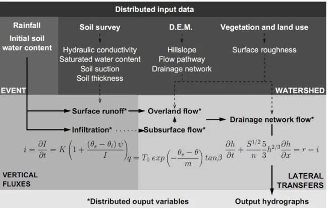
Following these observations the modelling approach chosen for the catchment set is the distributed model MARINE for flash flood forecasting [Roux et al., 2011] with subsurface flow modelling. It takes advantage of distributed forcing and soil spatial properties. The predominant factor that is considered to give rise to the stream hydrograph is represented by the topography: slope and downhill directions on a regular grid of squared cells. MARINE runs now on a various time step for calculation time reduction and is structured into three main modules (Figure 103). The two first represent soil saturation dynamics in MARINE model, governed by Green and Ampt infiltration model and subsurface flow in the soil superficial layer. The first module allows separating the precipitation into surface runoff and infiltration using the Green and Ampt model; the second module represents subsurface downhill flow with an approximation of the Darcy's law and the third one the overland flow (over hillslopes and in the drainage network): the transfer function component allows routing the rainfall excess to the catchment outlet using the kinematic wave approximation. Both infiltration excess and

saturation excess are represented within MARINE. Among the quantity of information about soil superficial layers, we derive soil thickness and texture maps for Rawls and Brakensiek soil classes definition, in particular for our model MARINE (Figure 102). Evapotranspiration is not represented since the model purpose was to simulate individual flood events during which such process is negligible. Bedrock is not taken into account in the governing equations of MARINE model since deep percolation is a poorly understood phenomenon and measurements to constrain a model are rare. But geology map is useful to analyze the flood simulation results, especially for comparative hydrology on several contrasted catchments.

Figure 103 : MARINE model structure, parameters and variables. Green and Ampt infiltration equation: infiltration rate i (m.s−1), cumulative infiltration I (mm), saturated hydraulic conductivity K (m.s−1), soil suction at wetting front ψ (m), saturated and initial water contents are respectively θs and θi (m3 m−3). Subsurface flow: local transmissivity of fully saturated soil T0 (m2s−1), saturated and local water contents are θs and θ (m3 m−3), transmissivity decay parameter is m (–), local slope angle β (rad). Kinematic wave: water depth h (m), time t (s), overland flow velocity u (m.s−1), space variable x (m), rainfall rate r (m.s−1), infiltration rate i (m.s−1), bed slope S (m.m−1), Manning roughness coefficient n (m−1/3.s).

This validated model formulation leads to good performances, with Nash-Sutcliffe and LNP criterions superior to 0.9 in most of the calibration events in the Cévennes region. Moreover, MARINE model parameters are calculated from soil surveys and remote sensed data and have some physical meaning. For a complete description of the MARINE model the reader can refer to [Roux et al., 2011].

5. EVENT MODEL SENSITIVITY AND ANALYSIS 5.1. GSA-GLUE approach

The highly non linear mathematical formulation of rainfall to runoff transform makes hydrological model response surface quite complex. The first step of the calibration consists in definition of a method that evaluates how well the model conforms to the observed system behaviour. But there is no consensus defining a criterion to appreciate model performance, and different objective functions can lead to identify different parameter combinations [Zin, 2002].

Besides we can distinguish methods that use a partitioning or the integrality of rainfall runoff chronics such as multiobjective optimization [Vrugt et al., 2009; Vrugt et al., 2003]. [Wagener

et al., 2003] propose the concept of dynamic identification with moving windows, or more

recently on sub periods characterized by similar hydrological behaviour [Choi and Beven, 2007].

This study is focused on a dataset composed of contrasted catchment flood responses [Garambois et al., 2012a]. The possibility of including several criteria for model performance evaluation is an interesting concept especially for flood modelling [Aronica et al., 2002;

Aronica et al., 1998; Werner, 2004]. The criteria introduced by [Roux et al., 2011], which in

addition to the classical normalized least squares considers features characterizing the flood peak (discharge value and time to peak) [Lee and Singh, 1998], is used:













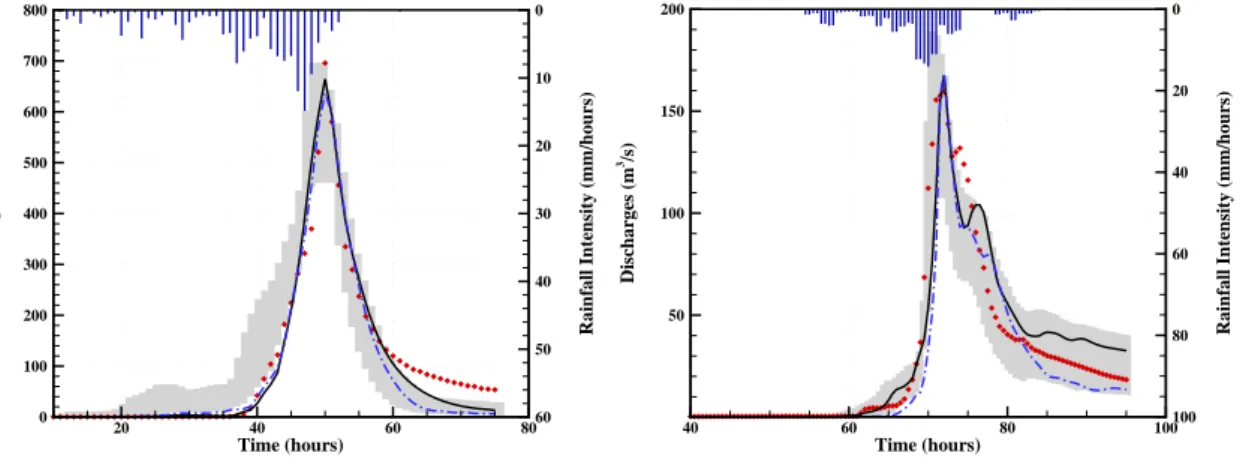
where Nobs is the number of observation data, Qs and Qo are respectively the simulated and the observed runoff, QPs and QPo are respectively the simulated and observed peak runoff, TPs and TPo are respectively the simulated and observed time to peak, TCo is the time of concentration of the catchment, α, β and γ are weights. This function grants importance to peak flow value and timing, which is particularly appropriate for MARINE model that focuses more on flash flood peak flow modelling than baseflow or recession. Moreover, event simulations with a high Nash can present a bad peak flow value and timing, which is why in the LNP cost function equal weights, are chosen. It reveals to be a correct compromise to explore the range of catchment flood behaviours since it leads to selects simulations that are satisfying from the flood forecaster point of view as shown by the two best simulations and the confidence interval on (Figure 104).

In order to avoid a model over-parameterization, spatial patterns of several parameters are derived from soil surveys and a unique correction coefficient is then applied to each parameter map. This approach has been chosen for three parameters, namely the distributed saturated hydraulic conductivity K, the lateral transmissivity T0 and soil thicknesses Z. The calibration procedure consists in estimating: three coefficients of correction one for the saturated hydraulic conductivities, named CK, another one for the lateral subsurface flow transmissivity CKSS and the last one for the soil thicknesses, named CZ, the Strickler roughness of the minor bed KD1 and the Strickler roughness of the overbank of the drainage network KD2. The choice of these parameters follows observations made during calibration process in the mediterranean region [Roux et al., 2011]. Concerning the transmisivity Kss the spatial variability is taken from the hydraulic conductivity map. Calibration parameters and variation range are reported in (Table 16). In practice, initial ranges of parameter values for Monte Carlo sampling are chosen with the intent of exploring a large range of model behaviours. Uniform parameter distributions within their range of variation are mainly used in lack of prior information. Each set of parameter values is then assigned a likelihood of being a simulator of the system, on the basis of the chosen likelihood measure. It is noted that the likelihood function and the threshold are subjectively determined and this was discussed by [Freer et al., 1996].

Parameter Description Min Max

Ck Correction coefficient of the hydraulic conductivities (-) 0.1 10

CZ Correction coefficient of the soil thickness (-) 0.1 10

CKss Correction coefficient of the soil lateral transmissivity (-) 100 10000

KD1 Strickler roughness coefficient of minor bed (m1/3.s-1) 1 40

KD2 Strickler roughness coefficient of the overbank (m1/3.s-1) 1 30

The generalized sensitivity analysis is performed following the method proposed by [Hornberger and Spear, 1981]. For each parameter αk the behavioural (B) and non-behavioural (B) simulations, according to the performance function and a threshold, and their distributions





fn k and fm

 

parameter is important to simulate the researched behaviour. The contrary is not always true. Indeed the distributions and can show no separation whereas the αk parameter can be crucial for the simulation because of correlations with other parameters. It is a necessary but not sufficient condition that parameters must be sensitive to be identifiable.

5.2. Event Calibrations

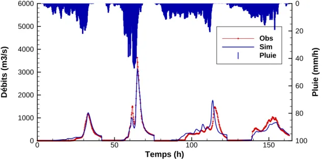
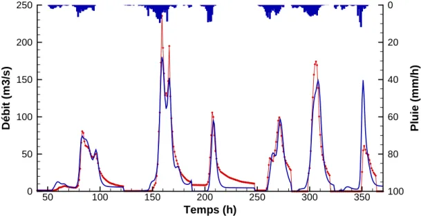
Confidence intervals and parameter posterior distribution functions are calculated with the GSA-GLUE method on a 5000 members Monte Carlo sample obtained with standard random generator. The threshold chosen on LNP for this method is 0.7 in order to be applicable to contrasted catchments. This choice appear reasonable since it ensures at least from 300 and on average 500 behavioural simulations to nearly thousand for the best simulated events for which LNP criterion can be superior to 0.95. This threshold is relatively high for our objective function in the case of flash flood as the narrow uncertainty interval can attest (Figure 104), the observations fall within this interval for most of the flood hydrograph. Moreover the uncertainty especially for peak flow is below 40% which is the order of high flow gauging error for some catchments and so the limit of acceptability as defined by [Blazkova and Beven, 2009]. We focus on peak dynamics, according to our cost function, and so it is not surprising if confidence interval does not fit the observed discharges for early rising limb or during recession (Figure 104, left). Let us remark that neither baseflow nor recession curves are used in MARINE model.

Time (hours) D is ch a rg es ( m 3/s ) Ra inf a ll Int ensi ty ( m m /ho ur s) 20 40 60 80 0 100 200 300 400 500 600 700 800 0 10 20 30 40 50 60 Time (hours) D is ch a rg es ( m 3/s ) Ra inf a ll Int ensi ty ( m m /ho ur s) 40 60 80 100 50 100 150 200 0 20 40 60 80 100

Figure 104: 2 best simulations (blue solid and blue dashed lines) and confidence interval for: (left) The Orbieu at Lagrasse (263 km²) 15/11/2005 flood event, performed with RA_Calibr radar rainfall data, 900 behavioural simulations; (right) The Tech at Pas-du-Loup (250 km²) 15/11/2005 flood event, performed with RG_Interp 5 rain gauges interpolated rainfall data, 480 behavioural simulations.

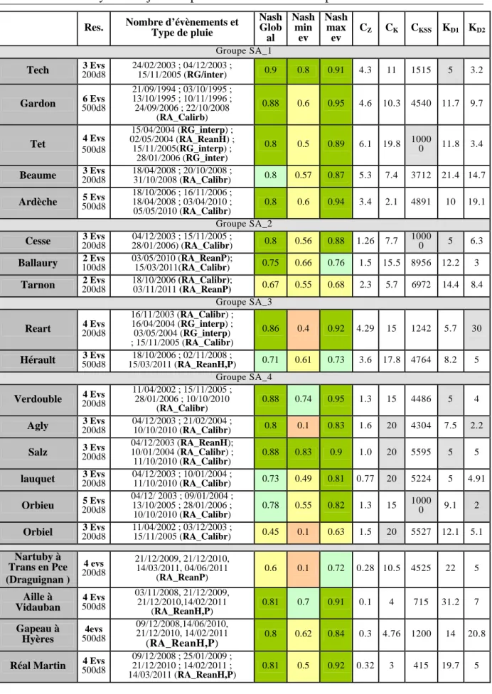
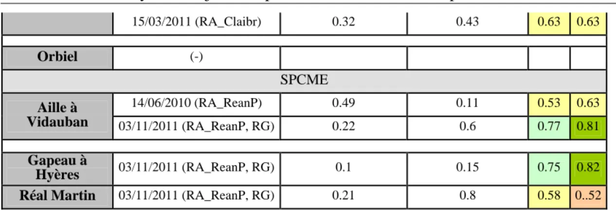
Following observations made during catchment calibration process Monte Carlo simulations are performed with different rainfall products for some questioning events in terms of QPE. A colour scale is proposed (Tableau 23) in order to help visual qualification of performance for event calibration with the different rainfall products (Table 41). Dark green is for the best Monte Carlo simulations for which GSA-GLUE is possible with respect to the hypothesis presented before. We can notice that Monte Carlo simulations give good results for all the catchments considered. Indeed, the four rainfall products give at least for each catchment one

flood with the best mark (i.e. (Nash, LNP) > 0,8) and two above (Nash, LNP)> 0,7. So, all the rainfall products can be appropriate for flash flood modelling purposes on these 11 Mediterranean catchments.

Besides, radar rainfall data seem to improve the possibility for flood modelling, since nearly all the floods simulated with either RA_Calibr (or RA_ReanP) give satisfactory performances with (Nash, LNP) above 0,7. The two ones that do not give correct results for RA_Calibr are very low flow events (06/02/2005 for the Orbieu and 10/04/2002 for the Têt). Interpolated raingauges from the dense measurement network give good results (Table 41). Let us remark that even a dense coverage with 5 raingauges for the Verdouble catchment (299 km²), do not give good modelling results for 08/01/1996 and 14/12/1995 events. Rainfall measurement network might not have seen the part of rainfall explaining catchment response for these two events.

Simulations in yellow or orange (Table 41), mostly for interpolated raingauges (RG_Interp) or RA_ReanH, are simulations that do not reproduce correctly observed hydrograph. A low LNP criterion often corresponds to simulations with underestimated peak flow but still good temporal dynamics and simulated peak time. In other word for the simulation marked in yellow and orange, the model water balance is not appropriate to reproduce at least the peak discharge order of magnitude, and so the water balance of a flood.

Most floods and catchments are correctly modelled with MARINE. Although parameter sets are sampled in relatively wide ranges in order to be able to reproduce different catchment behaviour, for several events the model water balance only engenders large underestimations, which addresses the question of which phenomenon leads to such an error on water conservation modelling?

In our modelling of rainfall to runoff conservation, among the possible sources of errors the three most important can be:

i. high flow gauging errors,

ii. model structure and parametric compensation (bedrock loss and evapotranspiration not simulated)

iii. QPE under or over estimates.

Parametric compensation is not taken into account explicitly, at least for water conservation. Most calibrations events are of comparable order of magnitude for a catchment, thus we can neglect gauging errors between events. In the following we focus on model parameter responsible for catchment storage capacity and water balance adjustments: CZ the spatial soil depth multiplicative constant. Indeed soil depth map multiplicative constant CZ controls catchment’s soil volume and can compensate runoff volume in a non negligible but still physical range (CZ





Performance condition for the couple (Nash, LNP) > 0.8 > 0.7 > 0.65 > 0.5 < 0.5 Colour correspondence

Catchment Verd ou b le Ce sse O r bi eu L au q ue t Agly Salz T ec h T ê t R eart O r bi e l Ballaury V_er d ou bl e C e sse Orbieu L_au q ue t Agly S a lz T ec h Têt R_eart Or_bi e l Ballaur y Verd ou b le Ce sse O r bi eu L au q ue t Agly S a lz T ec h Tê t R eart Orbiel B_a ll aur y Rainfall

type RA_Calibr RA_ReanP RG_Interp

03/11/2011 15/03/2011 10/10/2010 03/05/2010 RA_ReanH 11/04/2009 28/01/2006 15/11/2005 06/02/2005 13/10/2005 03/05/2004 15/04/2004 21/02/2004 10/01/2004 04/12/2003 16/11/2003 24/02/2003 11/04/2002 20/12/2000 10/06/2000 09/11/1999 03/11/1997 05/12/1996 30/11/1996 13/10/1996 01/02/1996 09/01/1996 14/12/1995 18/10/1994 23/12/1993 26/04/1993 26/09/1992 09/06/1992 08/05/1991 23/03/1991 12/02/1990 23/04/1988 03/04/1988 02/12/1987 06/11/1982 14/01/1982 27/02/1981 20/04/1981 14/04/1980

5.3. Catchment sensitivity to parameters

Monte Carlo calibrations for each catchment are performed under the identical mathematical and physical hypothesis and with the same data types, in order to be able to compare MARINE results and sensitivity between events and catchments. We will present inter event sensitivity to CZ in the following on each catchment, for the GSA-GLUE eligible events. (Table 42) shows parameter rank for each catchment, obtained by averaging Kolmogorov-Smirnov test values for all the events considered for GSA-GLUE analysis per catchment. Parameter rank and so model sensitivity to flow components varies in function of the catchment. Mean parameter rank, averaged for all the events and catchments are presented in (Table 42), CZ the spatial soil multiplicative constant is the most sensitive parameter on average whereas CKSS the lateral soil transmisivity is the less sensitive one, no clear tendency for the other parameter which sensitivity depends on catchment properties mainly. No clear trend for KD2 the overbank roughness which rank can go from 1 to 5 with an average of 2,9.

On average MARINE evaluated with LNP cost function is mostly sensitive to CZ and CK defining catchment storage capacity and infiltrability. These two sensitive parameters thus indicate that MARINE is mainly sensitive to runoff production dynamics and amount for flash flood events. Channel transfer function represented by main channel roughness and floodplain roughness is also important, whereas subsurface transfer appears less sensitive according to the model. Let us point the low interactions found between parameters with global sensitivity analysis.

Catchments CZ CK KD1 KD2 CKSS Tech 1 2 4 5 3 Tet 1 2 3 5 4 Verdouble 3 2 4 1 5 Agly 2 1 4 3 5 Salz 2 1 2 3 5 Lauquet 3 4 1 2 5 Orbieu 3 1 2 4 5 Cesse 1 2 3 5 4 Orbiel 3 4 2 1 5 Ballaury 2 5 3 1 4 Mean rank 2 2.7 2.9 2.9 4.5

Table 42: Mean catchment parameter ranking according to Dmax calculated for each parameter and event, Dmax being the maximal separation between f(_k B)and f(k B). Mean parameter rank is obtained by averaging each parameter rank for all the catchments.

5.4. Sensitivity to soil spatial soil depth and water volume control

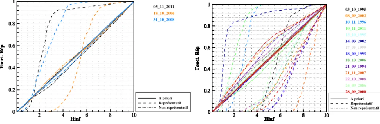
In this section we focus on CZ the spatial soil depth multiplicative constant, which on average reveals to be one of the most sensitive parameter of MARINE model for the 11 catchments. [Roux et al., 2011] show the sensitivity of MARINE to CZ on the Gardon d’Anduze catchment in the Cévennes. [Le Lay and Saulnier, 2007] with TOPMODEL, [Braud et al., 2010] with CVN and MARINE highlight that soil depth represents a strong control on flash flood response of catchments in the Cévennes. In the case of MARINE model applied to 11 Mediterranean catchments, we present CZ posterior distribution functions (PDFs) (Figure 106 to Figure 112), several events are plotted on one graph in order to compare PDFs. The following interpretations are based on multiple event calibration and validation, and parameter ranking also (Table 42). Event with similar sensitivity to CZ present similar averaged behaviours in terms of rainfall to runoff volume conservation.

CZ is the most sensitive parameter for Tech and Têt among the 9 others catchments (Figure 106), moreover the shape of PDFs shows that most of the behavioural simulations are for CZ values superior to 4, especially for the Têt (CZ>5). These two catchment’s sensitivities are corresponding to those of the Gardon d’Anduze catchment (Figure 105), which presents physiographic similarities, for example about 64% of the catchment area develops on metamorphic terrain. The substrate is made of shale and crystalline rocks overlain by silty clay loams - on 83% of the area - and sandy loam top soil [Chahinian and Moussa, 2007; Roux et al., 2011].

Cesse and Ballaury catchment are also very sensitive to CZ (Figure 107), and most of the behavioural simulations are for CZ values between 1 and 4. The physiographic and bedrock properties are complex for these catchments, Cesse is highly karstified [Nou et al., 2011]. For the Réart and Orbiel catchments presenting mixed and complex physiographic properties, most of behavioural simulations are for CZ values superior to 2 (Figure 108). Catchments from the ‘Corbières Mountains’ (Figure 109, Figure 110, Figure 111) are less sensitive to CZ than the previous catchments, and overall most of the behavioural simulations are for CZ values superior to 1. For those basins substrates develop mainly on primary era sedimentary bedrock (Table 38) overlain by loam and silty loam.

Bedrock loss and soil depth measurements uncertainty that are not accounted in the model and is certainly responsible for CZ values greater than one as suggested by [Castaings et al., 2007;

Roux et al., 2011]. Then the modeller has to increase soil volume and so storage capacity, to

produce a correct runoff volume for hydrograph formation given a QPE. Bedrock type and alteration might explain the large differences between catchment sensitivity and parameterization for CZ.

For each catchment most of the flood event recorded and simulated with Monte Carlo sampling are eligible for GSA-GLUE (Table 41), (Nash, LNP>0,8). The final objective is to find correct sets of events for gauged catchment calibration, in order to obtain a robust parameterization for regionalization purposes. Different rainfall products are used for each flood within a catchment to obtain plausible PDFs, i.e. sensitivity similarity. We use the following calibration and SA procedure that lead to select a rainfall product rather than another and to increase the number of events per catchment:

 Event sensitivity analysis with radar rainfalls (RA_Calibr) which is systematically available for the study zone, and also in a real time version for hydrological forecasts.

 PDF plotting and analyse.

 Raingauges or other radar rainfall product (RG_Interp, RA_ReanH, RA_ReanP) are then used with the view to increase the number of good GSA-GLUE candidates.

 Event selection, PDF plotting and analysis.

example because of availability. For a catchment, large dissimilarities for CZ sensitivity and unusually identified Cz value between events can be attributable to QPE errors under our hypothesis. With the wish to keep such an event for calibration phase, we look at the other PDFs obtained from different rainfall types if available for an event. For example on the Lauquet catchment, RA_Calibr gave good results first with the possibility to perform GSA-GLUE analysis, but the 04/12/2003 event PDF was not in agreement at all with the two other. The modelling performance is as good or better with RA_ReanH rainfall, and the sensitivity is now comparable to the other. This might indicate that QPE is better for hydrological modelling with RA_ReanH than with RA_Calibr for that catchment-flood. Calibration process only does not allow this discrimination. Several rainfall products are selected that way such as raingauges measurements for most events on Tech and Têt catchments even if radar data produced rather good modelling efficiencies.

For Verdouble (Figure 109, left) and Orbieu (Figure 110, left), first attempt modelling give good results in terms of PDF similarity. For both catchments, events before 2002 are modelled with RG_Interp, and the others with RA_Calibr or RA_ReanH.

Interpolated raingauge (RG_Interp) can give good results in terms of (Nash, LNP) and for PDF similarity in some cases: Orbieu and Tech, and some events on Verdouble, Cesse and Têt. This can be attributable to raingauge density and locations that seem to capture enough rainfall variability for satisfactory flood modelling but not for all the events. For example, despite its eligibility for GSA-GLUE, 28/01/2006 and 15/03/2011 (RG_interp) events on the Tech do not produce a PDF similar to the other. The same comment can be made for the event simulated with RG_interp for Salz catchment (10/06/2000, 30/11/1996). Moreover, let us remark that 26/09/1992 for the Salz which is a strong event (> 4 m3.s-1.km²), is not simulated correctly with raingauges, this highlight the need of radar data able to capture strong variabilities. On the contrary, PDF similarity does not exclude various hydrological behaviours for a particular catchment. For example, both small events and strong events that certainly activate different flow paths and runoff formation dynamics within a catchment, can present similar PDFs, as for 15/11/2005 for the Verdouble (3.3 m3.s-1.km²) and the Orbieu (2.65 m3.s-1.km²) or 02/12/1987 for the Cesse (2 m3.s-1.km²). This is true for both sensitive and less sensitive catchments to CZ. As an account we do not discriminate various catchment behaviours that can be caused by different rainfall spatial-temporal variability.

Different sensitivity and calibrated values of CZ coefficient between catchments can indicate different rainfall to runoff volume conservation relations for catchments. The PDF analysis is applicable to different rainfall types such as radar or interpolated raingauges data as results for Cesse, Verdouble and Orbieu catchments can attest. More generally for this catchment flood dataset, nearly half of the PDF selected are those obtained for radar rainfalls and half for interpolated raingauges, for all the catchments except Tech and Têt. It seems that Opoul radar data quality is quite variable in time and space with QPE errors sometimes affecting significantly hydrological modelling sensitivities and performances. Fortunately, the rather dense raingauge network allows a correct rainfall variability capture and so calibration event gathering. For the Tech and Têt catchments, raingauges give better results than radar data, maybe because they are the most far away catchments from the radar. In addition their highly marked topography with deep narrow valleys might disturb radar measurements.

Hinf Fo n ct . R ép 2 4 6 8 10 0 0.2 0.4 0.6 0.8 1 A priori Représentatif Non représentatif 03_10_1995 Hinf Fo n ct . R ép 2 4 6 8 10 0 0.2 0.4 0.6 0.8 1 08_09_2002 Hinf Fo n ct . R ép 2 4 6 8 10 0 0.2 0.4 0.6 0.8 1 13_10_1995 Hinf Fo n ct . R ép 2 4 6 8 10 0 0.2 0.4 0.6 0.8 1 17_05_1999 Hinf Fo n ct . R ép 2 4 6 8 10 0 0.2 0.4 0.6 0.8 1 18_09_1995 Hinf Fo n ct . R ép 2 4 6 8 10 0 0.2 0.4 0.6 0.8 1 18_10_2006 Hinf Fo n ct . R ép 2 4 6 8 10 0 0.2 0.4 0.6 0.8 1 21_09_1994 Hinf Fo n ct . R ép 2 4 6 8 10 0 0.2 0.4 0.6 0.8 1 22_10_2008 Hinf Fo n ct . R ép 2 4 6 8 10 0 0.2 0.4 0.6 0.8 1 24_09_2006 Hinf Fo n ct . R ép 2 4 6 8 10 0 0.2 0.4 0.6 0.8 1 28_09_2000

Figure 105 : Event posterior distribution functions (behavioural = dashed line, non behavioural = dash-dot line) for a Cévenol catchment: Gardon at Anduze (545 km²). Specific discharges range from 0.35 to 6.95 m3.s-1.km² for the events considered, all events are analyzed with (RA_Calibr) from Nîmes radar with the hypothesis of the present study for GSA-GLUE.

Hinf Fo n ct . R ép 2 4 6 8 10 0 0.2 0.4 0.6 0.8 1 A priori Représentatif Non représentatif 23_12_2000 Hinf Fo n ct . R ép 2 4 6 8 10 0 0.2 0.4 0.6 0.8 1 24_02_2003 Hinf Fo n ct . R ép 2 4 6 8 10 0 0.2 0.4 0.6 0.8 1 04_12_2003 Hinf Fo n ct . R ép 2 4 6 8 10 0 0.2 0.4 0.6 0.8 1 15_11_2005 Hinf Fo n ct . R ép 2 4 6 8 10 0 0.2 0.4 0.6 0.8 1 A priori Représentatif Non représentatif 15_04_2004 Hinf Fo n ct . R ép 2 4 6 8 10 0 0.2 0.4 0.6 0.8 1 02_05_2004 Hinf Fo n ct . R ép 2 4 6 8 10 0 0.2 0.4 0.6 0.8 1 15_11_2005 Hinf Fo n ct . R ép 2 4 6 8 10 0 0.2 0.4 0.6 0.8 1 28_01_2006 Hinf Fo n ct . R ép 2 4 6 8 10 0 0.2 0.4 0.6 0.8 1 15_03_2011

Figure 106: Event posterior distribution functions (behavioural = dashed line, non behavioural = dash-dot line), Tech at Pas du Loup (left) 04_12_2003 (RG_Interp), 15_11_2005 (RG_Interp), 24_02_2003 (RG_Interp); and Têt at Marquixane (right) 15_04_2004 (RG_Interp), 02_05_2004 (RA_ReanH), 15_11_2005 (RG_Interp), 28_01_2006 (RG_Interp), 15_03_2011 (RA_Calibr)

Hinf Fo n ct . R ép 2 4 6 8 10 0 0.2 0.4 0.6 0.8 1 A priori Représentatif Non représentatif 04_12_2003 Hinf Fo n ct . R ép 2 4 6 8 10 0 0.2 0.4 0.6 0.8 1 15_11_2005 Hinf Fo n ct . R ép 2 4 6 8 10 0 0.2 0.4 0.6 0.8 1 28_01_2006 Hinf Fo n ct . R ép 2 4 6 8 10 0 0.2 0.4 0.6 0.8 1 02_12_1987 Hinf Fo n ct . R ép 2 4 6 8 10 0 0.2 0.4 0.6 0.8 1 03_11_1997 Hinf Fo n ct . R ép 2 4 6 8 10 0 0.2 0.4 0.6 0.8 1 13_10_1996 Hinf Fo n ct . R ép 2 4 6 8 10 0 0.2 0.4 0.6 0.8 1 18_10_1994 Hinf Fo n ct . R ép 2 4 6 8 10 0 0.2 0.4 0.6 0.8 1 27_02_1981 Hinf Fo n ct . R ép 2 4 6 8 10 0 0.2 0.4 0.6 0.8 1 A priori Représentatif Non représentatif 03_05_2010 Hinf Fo n ct . R ép 2 4 6 8 10 0 0.2 0.4 0.6 0.8 1 15_03_2011

Figure 107: Event posterior distribution functions (behavioural = dashed line, non behavioural = dash-dot line), Cesse at Bize-Minervois (right), 04_12_2003 (RA_Calibr), 15_11_2005 (RA_Calibr), 28_01_2006 (RA_Calibr), 02_12_1987 (RG_Interp), 03_11_1997 (RG_Interp), 13_10_1996 (RG_Interp), 18_10_1994 (RG_Interp), 27_02_1981 (RG_Interp); Ballaury ay Banyuls, 15_03_2011 (RA_Calibr), 10_10_2010 (RA_ReanP)

Hinf Fo n ct . R ép 2 4 6 8 10 0 0.2 0.4 0.6 0.8 1 A priori Représentatif Non représentatif 03_05_2004 Hinf Fo n ct . R ép 2 4 6 8 10 0 0.2 0.4 0.6 0.8 1 15_11_2005 Hinf Fo n ct . R ép 2 4 6 8 10 0 0.2 0.4 0.6 0.8 1 16_04_2004 Hinf Fo n ct . R ép 2 4 6 8 10 0 0.2 0.4 0.6 0.8 1 04_12_2003 Hinf Fo n ct . R ép 2 4 6 8 10 0 0.2 0.4 0.6 0.8 1 16_11_2003 Hinf Fo n ct . R ép 2 4 6 8 10 0 0.2 0.4 0.6 0.8 1 A priori Représentatif Non représentatif 11_04_2002 Hinf Fo n ct . R ép 2 4 6 8 10 0 0.2 0.4 0.6 0.8 1 15_11_2005 Hinf Fo n ct . R ép 2 4 6 8 10 0 0.2 0.4 0.6 0.8 1 03_12_2003

Figure 108: Event posterior distribution functions (behavioural = dashed line, non behavioural = dash-dot line), Reart at Salleilles (left) ; 03_05_2004 (RG_Interp), 15_11_2005 (RA_Calibr), 16_04_2004 (RG_Interp), 04_12_2003 (RA_Calibr), 16_11_2003 (RA_Calibr); Orbiel at Villedubert (left), 11_04_2002 (RA_Calibr), 15_11_2005 (RA_ReanH), 03_12_2003 (RA_ReanH);

Hinf Fo n ct . R ép 2 4 6 8 10 0 0.2 0.4 0.6 0.8 1 A priori Représentatif Non représentatif 05_12_1996 Hinf Fo n ct . R ép 2 4 6 8 10 0 0.2 0.4 0.6 0.8 1 09_11_1999 Hinf Fo n ct . R ép 2 4 6 8 10 0 0.2 0.4 0.6 0.8 1 04_12_2003 Hinf Fo n ct . R ép 2 4 6 8 10 0 0.2 0.4 0.6 0.8 1 21_02_2004 Hinf Fo n ct . R ép 2 4 6 8 10 0 0.2 0.4 0.6 0.8 1 15_11_2005 Hinf Fo n ct . R ép 2 4 6 8 10 0 0.2 0.4 0.6 0.8 1 28_01_2006 Hinf Fo n ct . R ép 2 4 6 8 10 0 0.2 0.4 0.6 0.8 1 A priori Représentatif Non représentatif 04_12_2003 Hinf Fo n ct . R ép 2 4 6 8 10 0 0.2 0.4 0.6 0.8 1 15_03_2011 Hinf Fo n ct . R ép 2 4 6 8 10 0 0.2 0.4 0.6 0.8 1 15_11_2005 Hinf Fo n ct . R ép 2 4 6 8 10 0 0.2 0.4 0.6 0.8 1 21_02_2004

Figure 109: Event posterior distribution functions (behavioural = dashed line, non behavioural = dash-dot line), Verdouble at Tautavel (left) 05_12_1996 (RG_Interp), 09_11_1999 (RG_Interp), 04_12_2003 (RA_ReanH) 21_02_2004 (RA_Calibr), 15_11_2005 (RA_Calibr), 28_01_2006 (RA_Calibr); Agly at St Paul de Fenouillet (left), 04_12_2003 (RA_ReanH), 21_02_2004 (RA_ReanH), 15_11_2005 (RA_Calibr), 15_03_2011 (RA_Calibr)

Hinf Fo n ct . R ép 2 4 6 8 10 0 0.2 0.4 0.6 0.8 1 A priori Représentatif Non représentatif 05_05_1991 Hinf Fo n ct . R ép 2 4 6 8 10 0 0.2 0.4 0.6 0.8 1 09_01_1996 Hinf Fo n ct . R ép 2 4 6 8 10 0 0.2 0.4 0.6 0.8 1 12_02_1990 Hinf Fo n ct . R ép 2 4 6 8 10 0 0.2 0.4 0.6 0.8 1 23_12_1993 Hinf Fo n ct . R ép 2 4 6 8 10 0 0.2 0.4 0.6 0.8 1 26_04_1993 Hinf Fo n ct . R ép 2 4 6 8 10 0 0.2 0.4 0.6 0.8 1 28_01_2006 Hinf Fo n ct . R ép 2 4 6 8 10 0 0.2 0.4 0.6 0.8 1 15_11_2005 Hinf Fo n ct . R ép 2 4 6 8 10 0 0.2 0.4 0.6 0.8 1 10_10_2010 Hinf Fo n ct . R ép 2 4 6 8 10 0 0.2 0.4 0.6 0.8 1 09_01_2004 Hinf Fo n ct . R ép 2 4 6 8 10 0 0.2 0.4 0.6 0.8 1 A priori Représentatif Non représentatif 04_12_2003 Hinf Fo n ct . R ép 2 4 6 8 10 0 0.2 0.4 0.6 0.8 1 10_01_2004 Hinf Fo n ct . R ép 2 4 6 8 10 0 0.2 0.4 0.6 0.8 1 11_10_2010

Figure 110: Event posterior distribution functions (behavioural = dashed line, non behavioural = dash-dot line), Orbieu at Lagrasse (left) 05_05_1991 (RG_Interp), 09_01_1996 (RG_Interp), 12_02_1990 (RG_Interp), 23_12_1993 (RG_Interp), 26_04_1993 (RG_Interp), 28_01_2006 (RA_Calibr), 15_11_2005 (RA_Calibr), 10_10_2010 (RA_Calibr), 09_01_2004 (RA_Calibr) ; and Lauquet at St Hilaire (right) 04_12_2003 (RA_ReanH), 10_01_2004 (RA_Calibr), 11_10_2010 (RA_Calibr)

Hinf Fo n ct . R ép 2 4 6 8 10 0 0.2 0.4 0.6 0.8 1 A priori Représentatif Non représentatif 10_01_2004 Hinf Fo n ct . R ép 2 4 6 8 10 0 0.2 0.4 0.6 0.8 1 11_10_2010 Hinf Fo n ct . R ép 2 4 6 8 10 0 0.2 0.4 0.6 0.8 1 09_01_1996 Hinf Fo n ct . R ép 2 4 6 8 10 0 0.2 0.4 0.6 0.8 1 03_04_1988 Hinf Fo n ct . R ép 2 4 6 8 10 0 0.2 0.4 0.6 0.8 1 14_01_1982 Hinf Fo n ct . R ép 2 4 6 8 10 0 0.2 0.4 0.6 0.8 1 20_04_1981 Hinf Fo n ct . R ép 2 4 6 8 10 0 0.2 0.4 0.6 0.8 1 20_12_2000 Hinf Fo n ct . R ép 2 4 6 8 10 0 0.2 0.4 0.6 0.8 1 23_03_1991 Hinf Fo n ct . R ép 2 4 6 8 10 0 0.2 0.4 0.6 0.8 1 23_04_1988

Figure 111: Event posterior distribution functions (behavioural = dashed line, non behavioural = dash-dot line), Salz at Cassaignes (left) 10_01_2004 (RA_Calibr),11_10_2010 (RA_ReanP), 09_01_1996 (RG_Interp), 03_04_1998 (RG_Interp), 14_01_1982 (RG_Interp), 20_04_1981 (RG_Interp), 20_12_2000 (RG_Interp), 23_03_1991 (RG_Interp), 23_04_1988 (RG_Interp).

6. CATCHMENT PARAMETER SETS

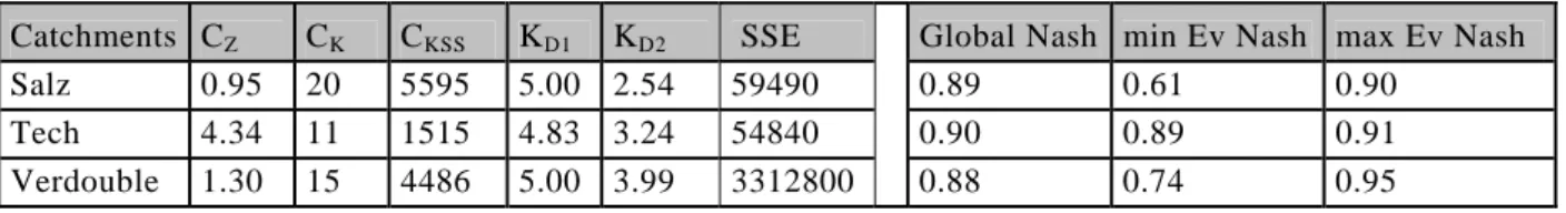
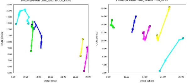
As stated before, hydrologic model calibration is a delicate problem given the complex response surface engendered by non linear formulation. The cost function choice transforms this into an optimisation problem. Contrarily to convex and quadratic surfaces characteristics of linear problems, optima in hydrology can present multiple convergence zones (multi modal), highly anisotropic curving, and singular points [Duan et al., 1992; Johnston and Pilgrim, 1976]. Moreover the problem becomes complex for event flash flood dedicated hydrologic model, when it is question to determinate catchment parameter sets able to describe a large panel of events and a fortiori various types of behaviours, and to compensate non stationary errors. In this section catchment calibration is performed for 3 catchments with several events and the rainfall data type selected with PDF similarity method. We use a minimization BFGS like algorithm called M2QN1 [Lemaréchal and Panier, 2000] and SSE criterion (Sum of Square Error) to calibrate the five sensitive parameters of MARINE model (Table 42). The algorithm is run for five random starting points in the parameter ranges defined in (Table 42). This multiple direction optimisation algorithm is used both for calibration and real time variational data assimilation within MARINE model [Castaings et al., 2009]. For this minimization technique, among the easy to implement criterion, the raw SSE criterion is more appropriate in opposition to the Nash that compares flow errors to the mean flow. The LNP criterion would be suitable for a multiobjective like calibration, but its implementation requires further work.

The aim here is not to discuss about calibration method which often converges to the same parameter combination from different starting points in the parameter space, but to illustrate the usefulness of PDF selection for rainfall analysis. Events are chosen among the GSA-GLUE candidates with similar PDFs. Besides, the events of different shape selected for calibration may represent some features of catchment behaviour.

We select three medium size catchments of 144, 250 and 299 km² (Figure 112 to Figure 114). Let us notice that 11/04/2002 calibration and 15/03/2011 validation events PDFs for the Verdouble (Figure 114) are similar to the other but not presented in the section above with a worry of rigor regarding the number of behavioural simulations. Indeed Monte Carlo best LNP are around 0.83 for those events but the number of behavioural simulations was judged insufficient.

Besides 15/03/2011 event on the Tech illustrates the benefits of this method. Indeed The CZ PDF of 15/03/2011 (RG_interp) event on the Tech, was not similar to the other and suggested QPE underestimation as confirmed by validation (Figure 113, right) and runoff coefficient (Table 44). Single calibration for this event give CZ values around 2.5. Moreover for this particular event now considered with (RA_Calibr) rainfalls, the CZ PDF comparison shows a