HAL Id: hal-03241947
https://hal.archives-ouvertes.fr/hal-03241947
Submitted on 29 May 2021
HAL is a multi-disciplinary open access
archive for the deposit and dissemination of
sci-entific research documents, whether they are
pub-lished or not. The documents may come from
teaching and research institutions in France or
abroad, or from public or private research centers.
L’archive ouverte pluridisciplinaire HAL, est
destinée au dépôt et à la diffusion de documents
scientifiques de niveau recherche, publiés ou non,
émanant des établissements d’enseignement et de
recherche français ou étrangers, des laboratoires
publics ou privés.
PHOENIX models across the HR-diagram
A Lançon, A Gonneau, K Verro, P Prugniel, A Arentsen, S Trager, R Peletier,
Y-P Chen, P Coelho, J Falcón-Barroso, et al.
To cite this version:
A Lançon, A Gonneau, K Verro, P Prugniel, A Arentsen, et al.. A comparison between X-shooter
spectra and PHOENIX models across the HR-diagram. Astronomy and Astrophysics - A&A, EDP
Sciences, 2021, 649, �10.1051/0004-6361/202039371�. �hal-03241947�
Astronomy
&
Astrophysics
https://doi.org/10.1051/0004-6361/202039371
© A. Lançon et al. 2021
A comparison between X-shooter spectra and PHOENIX models
across the HR-diagram
A. Lançon
1, A. Gonneau
2, K. Verro
3, P. Prugniel
4, A. Arentsen
5,1, S. C. Trager
3, R. Peletier
3, Y.-P. Chen
6,
P. Coelho
7, J. Falcón-Barroso
8,9, P. Hauschildt
10, T.-O. Husser
11, R. Jain
1, M. Lyubenova
12, L. Martins
13,
P. Sánchez Blázquez
14, and A. Vazdekis
8,91Université de Strasbourg, CNRS, Observatoire astronomique de Strasbourg, UMR 7550, 67000 Strasbourg, France
e-mail: [email protected]
2Institute of Astronomy, University of Cambridge, Madingley Road, Cambridge CB3 0HA, UK
3Kapteyn Astronomical Institute, University of Groningen, Postbus 800, 9700 AV Groningen, The Netherlands
4Centre de Recherche Astrophysique de Lyon (CRAL, CNRS, UMR 5574), Université Lyon 1, Ecole Nationale Supérieure de Lyon,
Université de Lyon, France
5Leibniz-Institut für Astrophysik Potsdam (AIP), An der Sternwarte 16, 14482 Potsdam, Germany 6New York University Abu Dhabi, PO Box 129188, Abu Dhabi, UAE
7Universidade de São Paulo, Instituto de Astronomia, Geofísica e Ciencias Atmosféricas, Rua do Matáo 1226, 05508-090 São Paulo,
Brazil
8Instituto de Astrofísica de Canarias, Vía Láctea s/n, 38200 La Laguna, Tenerife, Spain 9Departamento de Astrofísica, Universidad de La Laguna, 38205 La Laguna, Tenerife, Spain 10Hamburger Sternwarte, University of Hamburg, Gojenbergsweg 112, 21029 Hamburg, Germany
11Institut für Astrophysik, Georg-August-Universität Göttingen, Friedrich-Hund-Platz 1, 37077 Göttingen, Germany 12European Southern Observatory, Karl-Schwarzschild-Strasse 2, 85748, Garching, Germany
13NAT – Universidade Cruzeiro do Sul, Rua Galvão Bueno, 868, São Paulo, SP, Brazil
14Departamento de Física Teórica, Universidad Autónoma de Madrid, 28049 Cantoblanco, Spain
Received 8 September 2020 / Accepted 24 November 2020
ABSTRACT
Aims. The path towards robust near-infrared extensions of stellar population models involves the confrontation between empirical and
synthetic stellar spectral libraries across the wavelength ranges of photospheric emission. Indeed, the theory of stellar emission enters all population synthesis models, even when this is only implicit in the association of fundamental stellar parameters with empirical spectral library stars. With its near-ultraviolet to near-infrared coverage, the X-shooter Spectral Library (XSL) allows us to examine to what extent models succeed in reproducing stellar energy distributions (SEDs) and stellar absorption line spectra simultaneously.
Methods. As a first example, this study compares the stellar spectra of XSL with those of the Göttingen Spectral Library, which are
based on the PHOENIX synthesis code. The comparison was carried out both separately in the three arms of the X-shooter spectrograph known as UVB, VIS and NIR, and jointly across the whole spectrum. We did not discard the continuum in these comparisons; only reddening was allowed to modify the SEDs of the models.
Results. When adopting the stellar parameters published with data release DR2 of XSL, we find that the SEDs of the models are
consistent with those of the data at temperatures above 5000 K. Below 5000 K, there are significant discrepancies in the SEDs. When leaving the stellar parameters free to adjust, satisfactory representations of the SEDs are obtained down to about 4000 K. However, in particular below 5000 K and in the UVB spectral range, strong local residuals associated with intermediate resolution spectral features are then seen; the necessity of a compromise between reproducing the line spectra and reproducing the SEDs leads to dispersion between the parameters favored by various spectral ranges. We describe the main trends observed and we point out localized offsets between the parameters preferred in this global fit to the SEDs and the parameters in DR2. These depend in a complex way on the position in the Hertzsprung–Russell diagram (HRD). We estimate the effect of the offsets on bolometric corrections as a function of position in the HRD and use this for a brief discussion of their impact on the studies of stellar populations. A review of the literature shows that comparable discrepancies are mentioned in studies using other theoretical and empirical libraries.
Key words. stars: general – galaxies: stellar content – stars: atmospheres
1. Introduction
Stellar population studies based on the integrated spectra or col-ors of galaxies have a long history. Together with the studies of nearby resolved populations, they have allowed us to reach a broad understanding of the stellar contents of galaxies of dif-ferent types or environments and of their components. While it may not be critical to characterize each galaxy in detail to study the average evolution of the stellar mass across cosmic time (e.g.,
Madau & Dickinson 2014;Moutard et al. 2016), age and
metal-licity estimates become essential when studying the assembly of galaxy components; accurate interpretations of colors and spectral features are necessary to disentangle otherwise degen-erate properties such as age, metallicity, and extinction, to obtain absolute rather than relative values for these quantities, or to con-strain the stellar initial mass function based on integrated light. Such detailed investigations require population synthesis models to rest on robust stellar evolution calculations and on libraries A97, page 1 of31 Open Access article,published by EDP Sciences, under the terms of the Creative Commons Attribution License (https://creativecommons.org/licenses/by/4.0),
of stellar spectra with both accurate spectral features and accu-rate spectral energy distributions (SEDs). Indeed, the bolometric corrections associated with the SEDs determine the relative con-tributions of any type of star at any particular wavelength, and these contributions are key ingredients of the interpretation of the summed spectral features of the stellar population under scrutiny.
In this context, it is disturbing that it remains so difficult to combine optical and near-infrared (near-IR) studies of stel-lar populations. Attempts to match the colors of stel-large samples of galaxies from the near-ultraviolet (near-UV) to the near-IR have been found to leave significant residuals, sometimes lead-ing authors to discard near-IR data in part of their analysis
(Taylor et al. 2011). Star formation histories derived from
opti-cal and near-IR data separately, or from a given data set with different population synthesis models, still differ significantly
(Powalka et al. 2017;Baldwin et al. 2018;Dahmer-Hahn et al.
2018; Dametto et al. 2019; Riffel et al. 2019). A part of the
problem certainly lies in the theoretical modeling of advanced phases of stellar evolution, but it is also worth questioning the stellar spectral libraries. Indeed, if the balance between optical and near-infrared flux, for a given pattern of spectral features, is incorrect for individual stars, biases in the population synthesis models are inevitable.
Stellar spectral libraries can be either theoretical or empir-ical. In an ideal world, both would be equivalent. But this is a far-off target, and we are in the middle of a slow converging process that implies progress on both sides. Indeed, theoretical libraries cannot be tested without extensive empirical libraries, and empirical libraries cannot be used without stellar parameters, which are themselves estimated via comparisons with theoreti-cal spectral properties. For the purpose of checking the overall consistency of spectral features and SEDs, continuity across the wavelength range of photospheric emission, a reasonable spec-tral resolution and a good spectrophotometric calibration are keys.
The above requirements can be fulfilled with instruments such as the X-shooter spectrograph on the Very Large Tele-scope of the European Southern Observatory. The three arms of X-shooter, known as UVB, VIS, and NIR, together cover wave-lengths from the near-UV well into the near-IR. The instrument was used to construct the X-shooter Spectral Library (XSL;Chen
et al. 2014;Gonneau et al. 2020, hereafter PaperI), with the dual
purpose of testing synthetic spectral libraries and serving as a direct ingredient for stellar population modeling. In this article, we provide the results of a first confrontation of these spectra with an extensive collection of synthetic spectra, namely the Göttingen Spectral Library (GSL;Husser et al. 2013). Compar-isons with a few other model sets will follow and we encourage model-builders to repeat similar studies independently. Subse-quent papers will present population synthesis models based on XSL, as well as the de-reddened, merged UVB, VIS, and NIR spectra constructed for these (Verro et al., in prep.).
Our immediate aims are (i) to investigate to what extent stel-lar parameters based on optical absorption line spectra (Arentsen
et al. 2019, hereafter PaperII) lead to good matches between
the-oretical and empirical energy distributions over the wavelength range of X-shooter data and (ii) to determine to what extent the models are able to account for the global energy distribution of the data when the assumption that the parameters are those of PaperIIis relaxed. Side products of this study are (iii) a compar-ison between the parameters obtained from individual spectral ranges (i.e., the UVB, VIS and NIR arms of X-shooter), (iv) a validation of the relative flux calibration of the X-shooter data,
and (v) a quantitative estimate of the errors on bolometric correc-tions that may result from inconsistencies between SED-based and line-based parameter-estimates.
Considering the challenges of the modeling of cool stars, we expect to find the largest discrepancies between empirical and theoretical spectral energy distributions at low effective temper-atures. For the practical purpose of population synthesis, any such discrepancies translate into uncertainties in the fundamen-tal parameters associated with the empirical spectra. Issues that can be neglected to some extent when dealing with star and galaxy spectra in only a restricted spectral range, or with only low resolution SEDs, become more important to quantify when flux-calibrated spectra are used across optical to near-infrared wavelengths.
The main features of the GSL collection of synthetic spectra are recalled in Sect.2and those of the XSL data in Sect.3. We then specify the two methods used to confront the empirical and theoretical data sets with each other in Sect.4, and describe the results as a function of the position in the HR diagram in Sect.5. For reasons that will become clear later, we focus on the most significant trends and on the temperature regime between 4000 and 5000 K. Section 6 provides a comparison with other rela-tively recent confrontations between empirical and theoretical stellar spectra, a review of the limitations of GSL (many of which are common to a number of synthetic spectral libraries), and a brief discussion of the potential impacts of the trends we found, via bolometric corrections. The appendices provide a selection of additional figures; XSL-GSL comparison-figures for all the XSL spectra can be requested from the first author.
2. The models
The synthetic spectra used in this article are taken from Göttin-gen Spectral Library (GSL,Husser et al. 2013) in its version v21.
The comparison with the X-shooter Spectral Library was one of the motivations for the computation of that grid, which provides a dense coverage of the HR-diagram at several compositions and covers the near-UV to near-IR range of X-shooter spectra at an adequate spectral resolution. This series of synthetic spectra pro-vides a good representation of broad-band color-color relations of stars in the Milky Way (Figs. 2 and 22 ofPowalka et al. 2016); it also provide good matches to optical absorption line spectra at medium resolution (e.g.,Roth et al. 2018;Husser et al. 2016).
The underlying model atmospheres are obtained with version v16 of the PHOENIX code (Hauschildt et al. 1999), in spher-ical symmetry. This geometry is important in the low-gravity regime, where an atmosphere’s extension is not negligible com-pared to the stellar radius (Scholz 1985;Plez et al. 1992;Heiter &
Eriksson 2006). The models and synthetic spectra adopt the
equation of state and opacities referred to as PHOENIX-ACES, the calculation of which includes measured and theoretical lines lists by R. Kurucz as available in 2009 (>88 million metal lines and >1 billion molecular lines). PHOENIX models with these inputs were found to have a structure similar to that of MARCS models of the same period (see Sect. 7 ofGustafsson et al. 2008). Like many other large grids in the literature, the model spectra assume Local Thermal Equilibrium (LTE), which is a recognized limitation (Short & Hauschildt 2003;Lanz & Hubeny 2007).
The synthetic spectra are available on a grid of parameter space of which the four axes are the effective temperature (Teff),
the surface gravity log(g) (g in cm s−2), the metallicity [Fe/H]
(with respect to the solar abundances ofAsplund et al. 2009), and
Table 1. Parameter coverage of the GSL grid of synthetic spectra.
Variable Range Step size
Teff(K) 2300 . . . 7000 100
7000 . . . 12 000 200 12 000 . . . 15 000 500
log(g) −0.5 . . . +5 0.5 No 60 at high Teff
[Fe/H] −4.0 . . . −2.0 1.0
−2.0 . . . +1.0 0.5
[α/Fe] −0.2 . . . +0.6 0.2 Full grid only at
[α/Fe] = 0 and +0.6 the α-element enhancement [α/Fe]. The boundaries and sam-pling steps are summarized in Table1; we note that a few [α/Fe] ratios higher than listed are available but were not considered here. α-enhancements affect the abundances of O, Ne, Mg, Si, S, Ar, Ca and Ti. They are introduced at a given [Fe/H], hence they affect the overall metallicity Z of the models.
Spherical geometry introduces an extra degree of freedom compared to plane-parallel models. The adopted model masses are expressed as a simple function of log(g) and Teff (Fig. 1 of
Husser et al. 2013); they range from about 0.5 to about 5 M
along the main sequence, and reach values >10 M at high
tem-peratures and low gravities. Then surface gravity g determines the radius. The stellar structures account for convection using the mixing length theory of turbulent transport, with a mixing length parameter in the range [1, 3.5] that depends on Teff and
log(g).
Between 300 and 2500 nm, the synthetic spectra are com-puted with a sampling step ∆λ such that λ/∆λ ' 500 000. That such a high resolution is necessary for a good representation of empirical spectra of cool stars even at R = 3000 has been known for some time (e.g., Fig. 1 ofLançon et al. 2007). The micro-turbulent velocities adopted to determine individual line profiles in the calculations are taken proportional to the aver-age turbulent velocities of convection zones. They are typically around 1 km s−1 for Teff < 9000 K and reach a maximum of
about 3.5 km s−1 between 5000 and 6000 K at the lowest
grav-ities (Fig. 3 ofHusser et al. 2013). They drop to essentially zero above 10 000 K. The wavelengths of the synthetic spectra were converted from vacuum to air for comparison with the empirical spectra described below.
3. The X-shooter spectra
3.1. The sample
The X-shooter spectra used in this article are those of Data Release 2 of XSL (XSL-DR2, PaperII). Once carbon stars and incomplete spectra are excluded, the release contains data for 730 observations of 598 stars. Giants (on the red giant branch, on the asymptotic giant branch or in the red supergiant phase) represent ∼55% of these observations, dwarfs ∼35%, and the remainder of the spectra belong to subgiants, to horizontal branch or blue loop stars, or in a few cases to objects in other short-lived transition phases.
Fundamental stellar parameters have been estimated for 713 of these spectra in PaperII. The effective temperatures range from ∼3500 K to ∼38 000 K and the metallicities [Fe/H] from ∼−2.7 to supersolar (Fig. 1). The 17 stars for which Arentsen
et al.(2019) did not derive parameters are two late M dwarfs and
some of the coolest Mira-type variables in XSL.
5000 10000 15000 Te® (DR2) 0 1 2 3 4 5 lo g (g ) (D R 2 ) ¡2 ¡1 0 1 [F e= H ] (D R 2 )
Fig. 1.Parameters of the XSL dataset, as evaluated byArentsen et al.
(2019). Open symbols correspond to spectra for which at least one of the three X-shooter arms was not corrected for slit-losses.
Gonneau et al.(2020) flagged a number of spectra as
pecu-liar. We exclude three of these from the sample (X0214, X0248, X0424) because their energy distributions are obviously incom-patible with the models used here: X0214 and X0248 correspond to an Ae/Be star with a near-infrared excess due to circumstel-lar material, and X0424 to the combined emission of two stars. We further exclude the 6 hottest spectra of the remaining col-lection, whose estimated effective temperatures (>21 000 K) are well beyond those available in the model grid.
In the end, we use a total of 704 spectra with parameter esti-mates from PaperII and we extend the sample to 721 spectra (704+17) when the parameter estimates are not critical. We have not rejected long-period variable stars (LPVs) from our sample and figures, but they are clearly special cases for which we can-not expect good representations with synthetic spectra based on static atmosphere models (see Lançon et al. 2019, for prelimi-nary results of a dedicated study). The results highlighted in this paper focus on regions of stellar parameter space where these stars have little or no impact.
3.2. Properties of the spectra
The properties most relevant to the analysis in this article are the wavelength coverage of the spectra, the spectral resolution, the flux calibration, and the signal-to-noise ratio (S/N). The XSL-DR2 spectra are published in the rest-frame of each star, with wavelengths in air, and the exact wavelength coverage depends on the star observed. Before correction for radial velocity, the spectral ranges sampled by the UVB, VIS, and NIR arms of the X-shooter instrument are, respectively, 300–556, 533–1020, and 994–2480 nm. In practice, our analysis systematically excludes rest-frame wavelengths shorter than 400 nm for cool stars (Teff<
4200 K) and above 2.3 µm for all stars; other masked regions are mentioned in Sect.4.
As described in PaperI, the resolving power R = λ/∆λ is approximately constant across each arm, with R ' 9800, 11 600, and 8000, respectively in the UVB, VIS, and NIR arms. Because this study focuses on spectral energy distributions and major spectral features, we choose to perform all comparisons at a con-stant, reduced resolving power of either R = 500 or R = 3000. This smoothing also has the advantage of reducing any sensitiv-ity of the analysis to local residual wavelength calibration errors or variations in R. In practice, we first project the spectra onto an (oversampled) logarithmic wavelength scale and then convolve
Table 2. Standard deviations of the color-differences between XSL and external datasets (fromGonneau et al. 2020).
External Color Standard deviation Comments
reference σ(mag)
MILES (420–490) 0.03 0.056 incl. 7 outliers MILES (580–670) 0.02 0.032 incl. 3 outliers IRTF (J − H) 0.023 0.033 incl. 6 outliers IRTF (H − Ks) 0.019 0.029 incl. 4 outliers
2MASS (J − H) 0.032 0.050 incl. 2MASS errors 2MASS (H − Ks) 0.038 0.056 incl. 2MASS errors
Notes. The synthetic colors in the first two lines are measured in 600 or 800 nm-wide rectangular filters centered on the wavelengths indi-cated in the color-name, in nanometers. The 2MASS standard deviations listed each include six 4-σ outliers. The outliers are not the same for all colors.
each arm with an adequate Gaussian broadening function. To reduce computation times, we project the empirical and synthetic spectra, after smoothing, to a regular log-wavelength scale with ∼3 pixels per resolved element.
The XSL-DR2 data are available in two subsets, depending on whether or not a correction for slit-losses was applied to the fluxes. Among the 721 observations we consider, 597 are cor-rected for slit-losses in the UVB arm of X-shooter, 660 in the VIS arm, and 652 in the NIR arm. We focus on those spec-tra in our analysis. In PaperIsynthetic broad band photometry was used to compare colors of the XSL spectra with those of the MILES and IRTF spectral libraries, and with colors in the 2MASS point-source catalog. For the colors measured, the dis-tributions of the color-differences between the slit-loss corrected XSL spectra and other data typically have standard deviations of ∼0.03 mag (Table2), with a varying fraction of outliers (typi-cally 2–7% 4-σ outliers). The systematic offsets compared to the MILES and IRTF colors are smaller than 1%. The color-offsets with respect to 2MASS, also discussed in PaperI, are between 3 and 5.6%, but these values depend sensitively on the selected subsample, on the modeled contribution of telluric absorption to the filter transmission functions, and also on the adopted Vega spectrum; they are compatible with 2MASS photometric errors and systematics in the near-infrared synthetic photometry.
The S/N of the spectra are diverse, with typical values around 90 per original spectral pixel and above 100 after smoothing. We note that the computation of the initial noise spectra by the stan-dard X-shooter pipeline, starting from the original 2-dimensional echelle images, does not keep track of correlations introduced by the rectification and wavelength calibration. This impacts the noise-propagation through subsequent transformations such as our smoothing procedure2. Also, we are aware of a number of
cases in which the absolute level of the noise spectrum in one or the other X-shooter arm is dubious for unknown reasons (this is most obvious when the noise is overestimated). We must there-fore interpret any result that depends on the absolute noise levels with care. However, the noise spectra do contain the signature of the blaze function of the spectrograph, they show the lower S/N 2 Some of the issues with X-shooter noise spectra are described for the
UVB and VIS data inSchönebeck et al.(2014); the (partial) corrections suggested there are not implemented in the XSL pipeline, whose struc-ture depends on the architecstruc-ture of the original X-shooter instrument pipeline (distributed by the European Southern Observatory) until after the flatfielding and rectification of the spectra.
at both ends of the arm spectra, and they include a representa-tion of the errors induced by the correcrepresenta-tion for telluric absorprepresenta-tion (which is important in the near-infrared). Hence the inverse-variance based on the noise spectra provides useful, though not statistically optimal, weights for the pixel-by-pixel comparison of a given XSL spectrum with several synthetic spectra.
4. Data-model comparison methods
Our data-model comparisons aim at evaluating in which regions of stellar parameter space the theoretical spectra are able to reproduce the (low or intermediate resolution) spectral energy distributions across the wavelength range of X-shooter spectra. We do this first by adopting the stellar parameters of XSL-DR2 from PaperIIas they are; then we repeat the exercise without the strong assumption that the parameters are known a priori.
An essential point to remember is that only optical absorp-tion line spectra were exploited in PaperII: while applying the full-spectrum fitting code ULySS (Koleva et al. 2009), the authors discarded any information potentially carried by the SED, which was absorbed in a high order multiplicative poly-nomial of which the properties were not exploited. Discarding continuum information is a common procedure in stellar param-eter estimation work and also in full-spectrum fitting methods for the analysis of the integrated light of stellar populations. Here, on the contrary, the low resolution energy distributions of the XSL spectra are an essential piece of information we examine. Hence our data-model comparisons do not allow for any poly-nomial corrections. Only extinction is allowed to modify energy distributions.
4.1. Data-model comparison with the parameters of XSL-DR2 The first data-model comparison is performed for the XSL spec-tra for which the three parameters Teff, log(g), and [Fe/H] were
estimated in PaperII, and we adopt these values. As explained in detail in that article, these so-called “DR2-parameters” are tied to the estimated fundamental parameters of stars in previous empirical, optical spectral libraries (namely MILES and initially ELODIE; Prugniel & Soubiran 2001; Sánchez-Blázquez et al. 2006), which are themselves the result of a detailed literature compilation followed by extensive work to homogenize values obtained by different methods and authors (Cenarro et al. 2007;
Prugniel et al. 2011;Soubiran et al. 2016;Sharma et al. 2016).
Estimates of the [α/Fe] ratios are not systematically available for the XSL stars and literature values are dispersed. After a first exploration using four values of [α/Fe], we chose to base our analysis on synthetic spectra at [α/Fe] = 0 and +0.4, values that roughly represent the bulk of observed abundances in the Milky Way and Magellanic Clouds (Gonzalez et al. 2011;Nidever et al. 2020). The conclusions based on these two chemistries are sim-ilar, and the discussion further on explains why a more detailed approach would not be justified in this paper.
The discrepancies between the empirical and theoretical energy distributions are measured at low resolution (R = 500), using a normalized rms difference to quantify distance:
D = v u t 1 Nλ X λ FGSL λ − FXSLλ FXSL λ 2 . (1)
In this definition, Nλis the number of wavelengths accounted for
troublesome wavelength ranges (for instance regions with resid-uals from telluric absorption, ends of X-shooter arms that are affected by large flux calibration errors, and sometimes regions affected by line emission). FXSLis the smoothed XSL spectrum
and FGSL is the smoothed, optimally reddened and optimally
rescaled GSL spectrum under consideration. The extinction law
ofCardelli et al.(1989) is used with a standard ratio of total to
differential extinction, RV=3.1. For each GSL model,
redden-ing is optimized by minimizredden-ing D with respect to the extinction parameter AV. We allow only values of AV>−0.1, the negative
values being tolerated to limit edge effects that could be due to flux calibration errors in the XSL data. For each AV, the optimal
rescaling is re-evaluated.
In practice, the procedure is implemented in four variants that exploit four wavelength ranges. Each of the first three use only one of the X-shooter arms (UVB, VIS or NIR) to determine the best AV, while the fourth exploits all available wavelengths
jointly (it is labeled ALL). In the fourth case, we allow the opti-mization procedure to select the rescaling factors for the UVB, VIS, and NIR ranges independently of each other. If the col-lection of model spectra contains a perfect match to the data, reddening included, then all the four variants of the adjustment procedure should point to the same AV.
For very cool or highly reddened stars, the flux drops to zero at the blue end of the UVB arm and flux calibration errors may even produce negative fluxes. To avoid that D becomes exceed-ingly sensitive to regions of very low flux, we weight down the wavelengths ranges where the flux drops below 15% of the maximum flux of the arm.
The values of D can be interpreted as typical fractional dif-ferences between the best reddened model and the data. Flux calibration errors with 1-σ amplitudes equal to those listed in Col. 3 of Table2, if they are assumed to correspond to simple errors in the general slope of the spectra of one X-shooter arm, translate into changes in D of about 0.03 for each arm (with a slight dependence on the masked wavelength ranges used when computing D). Poor matches will be characterized by values of D larger than ∼0.06 as well as by inconsistent AV between
arms.
For the comparisons described in this section, we imple-mented an interpolation in the GSL grid before selecting the model nearest the parameters of a given XSL spectrum. The aim of the interpolation is to ensure that the discrepancy D between neighboring models in the theoretical grid remains smaller than the ∼0.03 that can result from flux calibration errors in the obser-vations. Interpolation does not change the main trends discussed in this paper which, when we choose to mention them, are larger than a model grid step on average; but it reduces the dispersion due to finite sampling of parameter space and hence raises the level of significance of the trends. Our interpolation reduced the step in Teff by a factor of 2 (typically from 100 K to 50 K), the
step in log(g) by a factor of 2 (from 0.5 to 0.25), and the step in [Fe/H] by a factor of 5 (from 0.5 to 0.1, or at low metallicity from 1 to 0.2). We used spline interpolation, in a local volume around the target parameters typically including 27 original grid points at a given [α/Fe]. We did not interpolate in [α/Fe].
4.2. The search for best-fit models
In the search for a best-fit model, Teff, log(g), [Fe/H], and [α/Fe]
are free parameters and the DR2-values of PaperIIare used only to initiate the optimization algorithm. Where useful, we include the 17 spectra with no associated parameters that were iden-tified in Sect. 3.1, and we assign them initial-guess effective
temperatures between 2300 and 3000 K, a surface gravity log(g) = 0 or 4.5, and a metallicity [Fe/H] = 0 (based on spectral type).
At any given [α/Fe], a subset of synthetic spectra centered on the DR2-parameters is selected. For each of these model spec-tra separately, a best-match extinction parameter AVis obtained,
using the standard extinction law ofCardelli et al.(1989) with RV=3.1. AV<−0.1 is prohibited. The fit-quality is measured at
resolution R = 500 or R = 3000 with a classical inverse-variance weighted χ2-difference between the reddened model and the
XSL-spectrum, or alternatively with the quantity D of the pre-vious section (Eq. (1)). If the best-fitting reddened model lies on the edge of the subset of models first selected, the subset is extended in the adequate direction until this is not the case (except on edges of the available model grid).
As in the previous section, the fitting procedure is imple-mented in four variants that exploit four wavelength ranges (UVB, VIS, NIR, and ALL). If the collection of model spec-tra contains a perfect match to the data, reddening included, then all these variants point to the same set of parameters.
When the figure of merit for each arm is the inverse-variance weighted χ2, the fourth variant of the fitting procedure, which we
refer to as the “global fit”, uses a combined-χ2based on the
val-ues obtained separately in each arm. There are numerous ways to proceed and we have implemented several, but since we restrict our discussion to major trends any choice that ensures a relatively even balance between the three arms leads to similar conclu-sions. The spectra of the three arms each contain comparable numbers of resolved spectral elements (∼104) and we choose to
give all three similar importance by calculating χ2global=1 3 χ2UVB min (χ2 UVB) + χ 2 VIS min (χ2 VIS) + χ 2 NIR min (χ2 NIR) , (2)
where the minima are taken over the subset of all reddened mod-els to which a given XSL spectrum was compared. To this latter purpose, the χ2-values per arm are initially saved for each
syn-thetic spectrum in the subset and for a broad range of values AV
including the values found best in each arm; the AVof the best
global fit, like the other parameters, can differ from each of the by-arm values. An advantage of this choice of χ2
global is its low
sensitivity to errors in the scaling of the noise spectrum that may affect one or the other arm; a caveat is the excessive weight that might be attributed to a spectral arm with poorer S/N.
The interpolation scheme of the previous section is also implemented here. We recall however that our point is not to re-evaluate stellar parameters per se, but to determine where in the HR-diagram good matches are possible or otherwise what the main trends in the discrepancies are. These conclu-sions are already apparent without interpolating. The procedure above produces a number of figures for eye inspection, of which examples are provided in AppendixA.
5. Results
5.1. The SEDs for the parameters of DR2
The differences between empirical and theoretical energy dis-tributions as measured by D (Eq. (1)) display systematic trends as a function of effective temperature, surface gravity, and metallicity, and we have therefore chosen to present them in HR-diagrams directly comparable to Fig.1. The maps for the four wavelength ranges we have considered (UVB, VIS, NIR, and ALL) are shown in Fig.2. For comparison, the values of D
5000 10000 15000 Te® (DR2) 0 1 2 3 4 5 6 lo g (g ) (D R 2) 0:01 0:02 0:05 0:1 0:2 0:5 D (U V B ) 5000 10000 15000 Te® (DR2) 0 1 2 3 4 5 6 lo g (g ) (D R 2) 0:01 0:02 0:05 0:1 0:2 0:5 D (V IS ) 5000 10000 15000 Te® (DR2) 0 1 2 3 4 5 6 lo g (g ) (D R 2 ) 0:01 0:02 0:05 0:1 0:2 0:5 D (N IR ) 5000 10000 15000 Te® (DR2) 0 1 2 3 4 5 6 lo g (g ) (D R 2 ) 0:01 0:02 0:05 0:1 0:2 0:5 D (A L L )
Fig. 2.Comparison between the low-resolution SEDs (R = 500) of XSL spectra and the nearest GSL spectrum, when adopting the fundamental parameters ofArentsen et al.(2019). Only extinction is allowed to modify the energy distribution of the theoretical spectra. The color-coding shows D (Eq. (1)), as measured in the UVB, VIS, and NIR arms and across the whole spectrum. Open symbols correspond to spectra for which no slit-loss corrections were applied. 1-σ flux calibration errors correspond to D ' 0.03 in each of the UVB, VIS, and NIR arms.
resulting solely from the finite sampling of parameter space in the theoretical spectral library can be examined in AppendixB. A selection of direct comparisons of the XSL and GSL low res-olution spectra, for the parameters of PaperIIas adopted in this section, can be found in AppendixC.
Strong systematic trends dominate the aspect of the four panels of Fig.2, with comparatively small local scatter. This pro-vides evidence that we are indeed measuring differences between empirical and theoretical stellar energy distributions rather than any dominant random errors in the XSL SEDs that previous examination of these data would have missed, or random errors due to the finite sampling of the model grid.
In the VIS and NIR arms, the theoretical SEDs are in excel-lent agreement with the empirical SEDs over vast regions of the HR diagram, corresponding roughly to Teff >4000 K. This is a
remarkable achievement of the GSL collection. The consistently low values of D over this part of parameter space (D 6 0.03) indicate that the photometric errors recalled in Table2 are not underestimated.
In the UVB arm, the model SEDs for the upper main sequence (Teff>5000 K) also agree with the data, albeit with
somewhat larger discrepancies D than in the VIS and NIR. With respect to the standard deviation σ associated with flux calibra-tion errors, the discrepancies are distributed between essentially 0 and about 2-σ (D ' 0.06). However, below ∼5000 K the mod-els disagree significantly with the UVB SEDs (D > 0.06) for
essentially all stars. They also disagree for the warm low-gravity stars in XSL. As a consequence, the energy distributions across all wavelengths are also in disagreement for these regimes.
Before discussing the general trends further, we briefly examine the most extreme outliers in Fig.2. Among the three data points near Teff=7500 K and log(g) = 0.5, the two lower
gravity ones are two observations of the same stars, a high metal-licity star with one of the highest extinction estimates in the sample (AV' 3); for the third data point, the literature and our
own estimates in Sect.5.2suggest the Teffof PaperIIis too high
by more than 1500 K (the DR2-parameters had been correspond-ingly flagged). Between 4000 and 5000 K, the spectra with the largest values of D(UVB) or D(ALL) are among those for which the observed fluxes are near zero below 400 nm, and the exact definition of the denominator in Eq. (1) matters. This is one of our reasons for focusing on typical situations and general trends instead of individual objects in this article.
Below 4000 K, it is notorious that stellar spectra are diffi-cult to model, for instance because of large surface convection cells, of variability, of the formation of dust grains. In the fol-lowing, we choose to concentrate on temperatures between 4000 and 5000 K, where these issues are in principle less severe. This regime contains stars with strong contributions to the inte-grated light of stellar populations over a broad range of optical and near-infrared wavelengths, which is a further reason for our interest.
The nature of the disagreement for stars between 4000 and 5000 K is illustrated with typical cases in Figs.C.5toC.11. There are systematic differences in spectral features (in particular in the UVB range), but our focus here is on energy distributions. What-ever wavelength range is used to estimate AV, discontinuities
appear in the figures at the limits between X-shooter’s spec-tral arms, showing that the energy distributions are not matched properly. Moreover, the steps are in the same direction for all the spectra shown (the examples are selected to be representative, only rare cases deviate from this behavior). Let us for instance examine Figs.C.7andC.11, where the extinction applied to the synthetic spectra is optimized using the VIS arm: the empirical spectra in the UVB and NIR fall off faster than the theoretical spectra when moving away from the VIS range. If the empiri-cal UVB and NIR spectra were resempiri-caled to connect to the VIS data smoothly, the merged spectrum would lack flux both in the UVB and NIR compared to the model. This trend is more obvi-ous at low metallicities (Fig.C.7) than at near-solar metallicity (Fig.C.11).
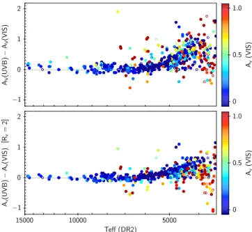
Another manifestation of the mismatch between empirical and theoretical SEDs is seen when comparing the extinction esti-mates obtained separately from the UVB and the VIS data: Fig.3
shows that below about 5000 K, AV(UVB) is in general larger
than AV(VIS). Both also tend to exceed AV(NIR), but because
of the wavelength dependence of extinction laws, AV(NIR) is
more sensitive to flux calibration errors and that trend is more dispersed. In brief: when using the UVB arm for the fit, a large AVis preferred and the theoretical spectrum has excess flux in
the NIR compared to the observations; when using the NIR arm for the fit, a small AVis preferred and the theoretical spectrum
has excess flux in the UVB compared to the observations. Three hypotheses come to one’s mind immediately: (i) either the extinction law is inadequate (it should rise more steeply towards the ultraviolet than the steepest law we explored), (ii) or the models lack opacities with a more severe deficit at shorter wavelengths, (iii) or the parameters in PaperIIare systematically offset for some other reason from those that would provide good fits with the GSL library.
Proposition (i) is unlikely, considering what is known about extinction in the Local Universe (Schlafly et al. 2016). It would also imply a correlation between the difference AV(UVB)−AV(VIS) and a mean estimate of extinction which,
if present at all, is weak in our data. Propositions (ii) and (iii) on the other hand are reminiscent of previous studies with various collections of synthetic and empirical spectra. To test proposi-tions (ii) and (iii) further, the results of the free search for the best-fit GSL match to each XSL observation are needed and we therefore postpone discussions to Sects.5.2and6.
We complete this part with a brief comment on the [α/Fe] ratio. The results shown in Figs. 2 and 3 combine estimates obtained with [α/Fe] = 0 and [α/Fe] = +0.4. Outside the range of parameters covered by the α-enhanced models, that is for Teff >8000 K, Teff <3500 K, log(g) < −0.1 or [Fe/H] > +0.1,
solar abundances were used. Elsewhere, we decided that the α-enhanced model was favored over the solar one when that change in abundances reduced D (UVB) by at least 0.01, without degrad-ing D (VIS), D (NIR), D (ALL) or | AV(UVB) − AV(VIS) |
sig-nificantly. The XSL-spectra favoring α-enhanced models are those of metal-poor giants, as expected from statistics in the Milky Way. Eye-inspection of the superimposed empirical and theoretical spectra with solar and with α-enhanced abundances, be it at R = 500 or R = 3000, then confirms the better match of the Ca II lines or the Mg I triplet (which are deeper in α-enhanced models) and the CH and CN bands (which are shallower in
5000 10000 15000 Te® (DR2) ¡1 0 1 2 AV (U V B )¡ AV (V IS ) 0 0:5 1:0 Av (V IS ) 5000 10000 15000 Te® (DR2) ¡1 0 1 2 Av (U V B )¡ Av (V IS ) [Rv = 2] 0 0:5 1:0 Av (V IS )
Fig. 3.Difference between the extinction estimates obtained with the UVB and VIS segments of the XSL data, from the comparison with GSL energy distributions when adopting the stellar parameters of
Arentsen et al.(2019). Top: standard extinction law (Rv = 3.1). Bottom: extreme extinction law (Rv = 2).
α-enhanced models because enhanced O captures a larger frac-tion of the available C). However, the effect of accounting for α-enhancement produces only very small changes in Fig.2, that the untrained eye would not even notice. The trends discussed above are unchanged.
In summary, the SEDs of the GSL models agree well with the SEDs of XSL, for the parameters of PaperII, over wide parts of the HR-diagram. But there is statistically significant system-atic disagreement below ∼5000 K, and for luminous warm stars (though with lower significance due to smaller numbers).
In the following section, we relax the assumption that the fundamental parameters are known and we search for the best-fitting model with that extra freedom. If models can be found that match the SEDs to within the errors (in the data and due to the discrete grid), we would be facing a classic parameter calibration problem: the reference libraries used in PaperII and GSL are different, and this may lead to offsets in derived parameters. It would remain to be determined which calibration is more robust. If adequate models cannot be found in certain parts of the HR-diagram, then these should be regions on which to focus future efforts in stellar spectral synthesis.
5.2. Best-fit model SEDs for each XSL spectrum
When the stellar parameters are free, better matches with GSL energy distributions can be obtained in the critical regions of the HR-diagram identified above. D now takes values between 0.03 and 0.06 for effective temperatures between 4000 and 5000 K (Fig. 4). Such values, taken individually, would be consistent with flux calibration errors at the 2 σ level. In fact a part of the discrepancies are due to local spectral features, and hence the part of D associated with the general low resolution energy distribution is even smaller than these 2 σ.
However the homogeneous behavior of the numerous data points below 5000 K in Fig.4 tells us that the values of D are not the result of random errors. Systematic discrepancies are still present. Despite the free exploration of parameter space, we must
5000 10000 15000 Te® (DR2) 0 1 2 3 4 5 6 lo g( g ) (D R 2 ) ¡0:02 ¡0:01 0 0:01 0:02 D (A L L; b es t m at ch ) ¡ D (A L L; D R 2 ) 5000 10000 15000 Te® (DR2) 0 1 2 3 4 5 6 lo g( g ) (D R 2 ) 0:01 0:02 0:05 0:1 0:2 0:5 D (A L L; b es t m at ch )
Fig. 4. Top: change in the discrepancy measure D (Eq. (1)) when, instead of adopting stellar parameters fromArentsen et al.(2019), the parameters are freely optimized. The data points are located in the diagram according to the DR2-parameters of Arentsen et al. (2019) The symbol color maps the difference between the best-fit value of D (Eq. (1)) and its value for the DR2-parameters. Bottom: discrepancy D for the best-fit stellar parameters (to be compared to the bottom right panel of Fig.2, where the parameters of Arentsen et al.(2019) were assumed). Complete versions of these figures, with one panel per arm, are available in Figs.D.1andD.2.
conclude that it remains difficult to reproduce both the spectral features and the low-resolution SEDs of the cool stars simultane-ously below 5000 K. Below, in Sect.5.2.1, we clarify the nature of the systematic discrepancies seen between the models with the best-fitting SEDs and the observations, where such discrep-ancies are present. Subsequently, in Sect.5.2.2, we quantify how the parameters of the best-SED models obtained here compare to those of PaperII.
5.2.1. Residual differences between best-SED models and XSL spectra
When the purpose is to find the best theoretical match to a given observation (as opposed to comparing the quality-of-fit for different observations), inverse-variance weighted χ2
val-ues are a more appropriate figure of merit than D, which gives low-flux regions at short wavelengths too much weight. For the sake of validation, we have performed all calculations with the two methods. The directions of the trends are unchanged, but amplitudes of the differences between the parameters from optimization and the parameters in PaperII depend on the weighting, in the sense that slightly larger differences are found on average when using D, than when using the inverse-variance
weighted χ2. In the following, we restrict the figures presented to
those obtained with the weighted χ2. We focus on temperatures
between 4000 and 5000 K.
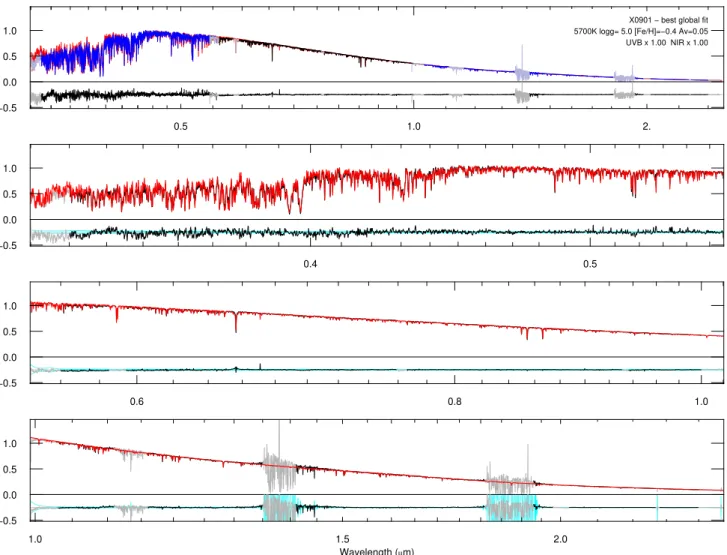
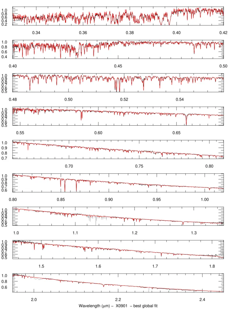
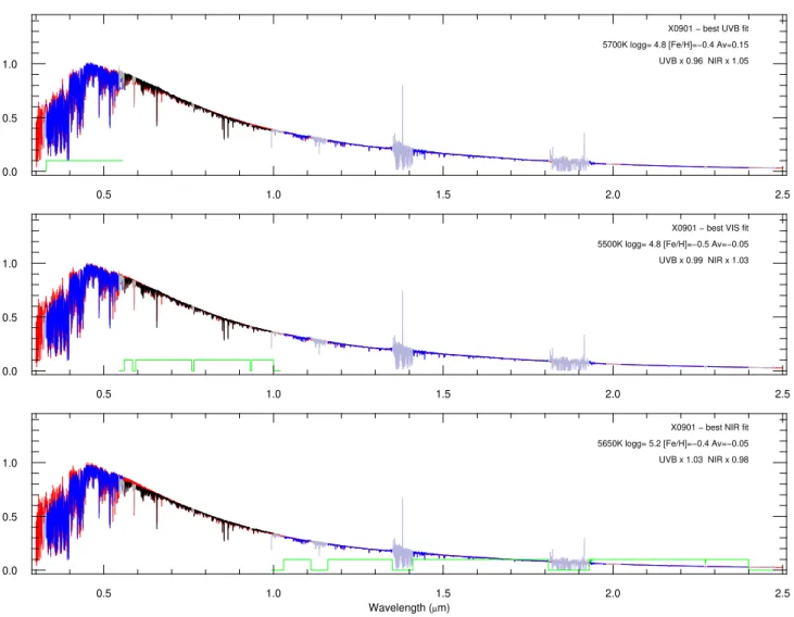
Examples of matched spectral energy distributions, based on fits performed at R = 500 by minimizing the inverse-variance weighted χ2across all available wavelengths (Eq. (2)), are shown
in Figs.5 and6respectively for relatively metal-poor and rela-tively metal-rich stars, with effective temperatures between 4000 and 5000 K according toArentsen et al.(2019). The energy dis-tributions from the near-UV to 2.4 µm are reproduced well for the new sets of stellar parameters indicated in the panels (com-pare with Figs.C.5andC.9). The residuals are roughly flat on average and the three arms in general connect naturally. In the near-IR, where the main low-resolution features are the shape of the H-band (set by continuous H− opacities) and the CN band
near 1.1 µm, excellent agreement with the observed shapes are obtained.
However, in this temperature range it is clear that the improvement in the SEDs does not always come with a good match of all the spectral features. The local features in the resid-uals are of varying amplitude but are generally highly significant (the S/N per resolved element is of several hundred at R = 500). They are not random but correspond to features in the spectra. There is some natural dispersion in the properties of the residu-als and we cannot provide an exhaustive description; the points we mention are those for which we have enough cases to consider they are systematic trends.
A striking first impression is that the UVB residuals would not satisfy any expert of stellar parameter estimates. They are clearly larger than those one can expect to achieve when fitting spectra over the traditional optical range (400–700 nm) when allowing for a polynomial correction of the continuum. They are also significantly larger than those we obtain with GSL when fit-ting only the UVB range with reddened models, instead of ALL wavelengths. In the VIS and NIR ranges, the features are intrinsi-cally weaker than in the UVB, and the physical natural variance is smaller between 4000 and 5000 K. The tension between the SED and the spectral features is still present to some extent, but weaker.
In luminous metal-poor giants (top rows of each panel of Fig. 5), the best-SED models tend to display a deeper G-band (CH molecule, 0.55 µm) than the observations. A fit restricted to the UVB arm would be able to eliminate this issue, but at the cost of degrading the panchromatic SED. At warm enough tem-peratures in the range considered, the metal-poor models display hydrogen lines, which for the best-SED tend to be too weak in the Balmer series but too deep in the near-IR Brackett series.
At higher giant-branch gravities (log(g)'2), an interesting trend appears across the UVB spectrum of metal-poor giants (middle rows in the upper right panel of Fig.5): the largest resid-uals take the shape of positive features at wavelengths longer than 0.49 µm, while it is the opposite below 0.43 µm. A closer look shows that the largest residual differences at the red end of the UVB arm correspond to strong metal lines, that are too deep in the best-SED models; this suggests that the constraints from the panchromatic SED pull the fit towards high metallicities. At the blue end of the UVB, the largest residuals are not associ-ated with strong lines, but are more broadly distributed. For main sequence stars (last rows in the panels of Fig.5), the largest resid-uals below 0.43 µm correspond to regions in between the deepest spectral features.
Moving to higher metallicities (Fig. 6), the trends just described for gravities log(g) & 2 remain present. The multitude of lines of molecular and atomic species makes it difficult to
X0232 − best global fit 4500K logg= 0.0 [Fe/H]=−2.4 Av=0.40 UVB x 1.06 NIR x 1.03
−0.5 0.0 0.5 1.0
X0393 − best global fit 4250K logg= 0.5 [Fe/H]=−2.4 Av=−0.05 UVB x 0.76 NIR x 0.99
−0.5 0.0 0.5 1.0
X0258 − best global fit 4350K logg= 1.5 [Fe/H]=−0.4 Av=0.15 UVB x 1.04 NIR x 1.00
−0.5 0.0 0.5 1.0
X0705 − best global fit 4750K logg= 2.0 [Fe/H]=−0.3 Av=0.75 UVB x 1.01 NIR x 0.96
−0.5 0.0 0.5 1.0
X0572 − best global fit 4600K logg= 5.2 [Fe/H]=−1.2 Av=0.00 UVB x 1.00 NIR x 1.00
−0.5 0.0 0.5 1.0
X0906 − best global fit 4100K logg= 5.5 [Fe/H]=−2.4 Av=0.05 UVB x 1.01 NIR x 1.02 1.0 2. 0.5 −0.5 0.0 0.5 1.0 Wavelength (µm) −0.5 0.0 0.5 1.0 −0.5 0.0 0.5 1.0 −0.5 0.0 0.5 1.0 −0.5 0.0 0.5 1.0 −0.5 0.0 0.5 1.0 0.4 0.5 −0.5 0.0 0.5 1.0 Wavelength (µm) −0.5 0.0 0.5 1.0 −0.5 0.0 0.5 1.0 −0.5 0.0 0.5 1.0 −0.5 0.0 0.5 1.0 −0.5 0.0 0.5 1.0 0.6 0.8 1.0 −0.5 0.0 0.5 1.0 Wavelength (µm) −0.5 0.0 0.5 1.0 −0.5 0.0 0.5 1.0 −0.5 0.0 0.5 1.0 −0.5 0.0 0.5 1.0 −0.5 0.0 0.5 1.0 1.0 1.5 2.0 −0.5 0.0 0.5 1.0 Wavelength (µm)
Fig. 5.Typical comparisons between XSL and best-match GSL energy distributions for stars with relatively low metallicities according to XSL DR2 and with DR2-Teffbetween 4000 and 5000 K. The comparisons are shown for the parameters that minimize the combined inverse-variance
weighted χ2 over all wavelengths (Eq. (2)). The upper left panels show all wavelengths at R = 500, the other panels are zooms into these same
comparisons, at R = 3000. The best-match synthetic spectra are in red; the empirical spectra in black, except in the upper left panel where they are shown in blue, black, and blue for the UVB, VIS, and NIR arms of X-shooter. Below each spectrum, the residuals are shown together with positive and a negative version of the XSL error spectrum (cyan). Gravity increases from top to bottom: HD 165195 (X0232), HD 1638 (X0258), NGC 68381037 (X0705), LHS 1841 (X0572), LHS 343 (X0906). Compare with Fig.C.5.
emphasize any other feature specifically. By letting the eye slide over the residuals presented, it can be seen that their features repeat (within a given regime of the HR diagram). The discrep-ancies are mostly systematic, rather than random. The calcium triplet for instance, around 0.86 µm, is usually too strong in the best-SED model for giants (the SED favoring [α/Fe] = 0 at solar-like metallicities), while it is well matched in the dwarfs.
The tension between the SED and the spectral features also manifests in the sensitivity of the best-fit parameters to the wavelength range considered in the comparison. For instance,
∆AV≡ AV(UVB)−AV(VIS) still is positive on average between
4000 and 5000 K, with 80% of the values spread between 0 and 0.8 (Fig. 7; compare with Fig. 3). This apparent temperature-dependence of ∆AVis due primarily to mismatches in the UVB
arm, where the density of strong spectral lines is largest. As described above, the simultaneous fit to all three arms produces residual features in the UVB with a systematic sign-difference between the blue end and the red end of that arm. A larger extinc-tion in the UVB would help reduce these residuals, and this happens in fits that do not use the VIS and NIR constraints. On
X0314 − best global fit 4800K logg= 0.0 [Fe/H]= 0.9 Av=−0.05 UVB x 1.81 NIR x 1.26
−0.5 0.0 0.5 1.0
X0504 − best global fit 4300K logg=−0.2 [Fe/H]=−1.1 Av=0.10 UVB x 1.04 NIR x 1.01
−0.5 0.0 0.5 1.0
X0563 − best global fit 4600K logg= 1.0 [Fe/H]= 0.0 Av=0.50 UVB x 1.00 NIR x 1.04
−0.5 0.0 0.5 1.0
X0698 − best global fit 4500K logg= 2.5 [Fe/H]= 0.8 Av=0.55 UVB x 0.99 NIR x 1.05
−0.5 0.0 0.5 1.0
X0739 − best global fit 4950K logg= 4.8 [Fe/H]= 0.6 Av=0.10 UVB x 1.07 NIR x 1.18
−0.5 0.0 0.5 1.0
X0560 − best global fit 4800K logg= 4.8 [Fe/H]= 0.8 Av=0.25 UVB x 1.04 NIR x 1.03 1.0 2. 0.5 −0.5 0.0 0.5 1.0 Wavelength (µm) −0.5 0.0 0.5 1.0 −0.5 0.0 0.5 1.0 −0.5 0.0 0.5 1.0 −0.5 0.0 0.5 1.0 −0.5 0.0 0.5 1.0 0.4 0.5 −0.5 0.0 0.5 1.0 Wavelength (µm)
Fig. 6.Typical comparisons between XSL and best-match GSL energy distributions for stars with relatively high metallicities according to XSL DR2 and with DR2-Teffbetween 4000 and 5000 K. The comparisons are shown at R = 500, for the parameters that minimize the combined
inverse-variance weighted χ2over all wavelengths (Eq. (2)). Gravity increases from top to bottom: HD 50877 (X0314), BBB SMC 104 (X0504), HD 44391
(X0563), 2MASS J18351420-3438060 (X0698), HD 218566 (X0739), HD 21197 (X0560). In the case of X0504, the best-match metallicity is lower than the DR2-value (−0.6), which had justified its presence is this subset of spectra. Compare with Fig.C.9.
5000 10000 15000 Te® (DR2) ¡2 ¡1 0 1 2 Av (U V B ) ¡ Av (V IS ) 0 0:2 0:4 0:6 0:8 1:0 Av (V IS )
Fig. 7.Same as Fig.3, but for the parameters and extinction that min-imize the inverse-variance weighted χ2-difference between models and
data in the UVB and VIS arms of X-shooter.
average, the extinction estimate based on the VIS arm compares well with the extinction evaluated from the three arms together.
In the comparison between parameters preferred by the dif-ferent arms of the spectrograph, the effects of degeneracies are seen strongly. For the sample as a whole, the difference ∆AV
cor-relates positively with the corresponding differences in Teffand
in [Fe/H] obtained using the UVB or the VIS arm, as expected from the notorious effects on Teffand AVon spectral slopes, and
from the need to compensate a higher Teffwith higher metallicity
in order to obtain spectral features of similar strength. How-ever, this hides a more complex dependence on position in the HR diagram and on metallicity. A few examples are given in AppendixE.
We find no significant correlation between ∆AV and
AV(ALL) or [AV(UVB)+AV(VIS)]/2 for the sample as a whole,
which would have been the most evident indication of an inad-equate extinction law. Nevertheless, we repeated the fits with an extinction law with a steeper rise in the UV, using RV=2 instead of RV= 3.1 in the parametric description ofCardelli et al.(1989).
As expected, RV=2 reduced ∆AVon average for giants between
4000 and 5000 K3, but without eliminating the positive average.
The other region of the HR diagram where our sample has high extinctions corresponds to luminous warm stars. Here, switch-ing to the steeper RVtends to increase the discrepancies ∆AV
between UVB and VIS estimates.
5.2.2. Systematic differences between best-SED parameters and those based on ULySS and MILES or ELODIE As discussed above, the models that reproduce the SEDs of the XSL-spectra best are not always those with the parameters derived by comparison of the absorption line spectra with the empirical libraries MILES or ELODIE. In a small number of cases, this can be traced back to an outlier-type failure of the analysis of the optical spectra, but this is not our main point here. On the contrary, we focus on generic trends, that systematically affect stars of a given part of parameter space and that withstand errors on individual parameters.
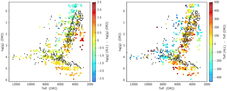
Gravity and temperature. A synthetic view of the differ-ences between the parameters Teff and log(g) of PaperII and
those obtained from the comparison with (reddened) theoreti-cal spectra (at R = 3000), is presented in the HR-diagrams of Fig. 8. Compared to the positions assigned in PaperII in Teff
and log(g) (black dots), the parameters assigned via the joint comparison of the three arms to GSL-spectra are systematically more dispersed (colored points). More dispersion is expected 3 Not below 4000 K, where the fits are poor and dispersion washes out
2000 4000 6000 8000 10000 12000 Te® (DR2) 0 1 2 3 4 5 6 lo g (g ) (D R 2 ) ¡2:5 ¡2:0 ¡1:5 ¡1:0 ¡0:5 0 0:5 1:0 1:5 2:0 2:5 lo g (g ) (A L L ) ¡ lo g (g ) (D R 2) 2000 4000 6000 8000 10000 12000 Te® (DR2) 0 1 2 3 4 5 6 lo g (g ) (D R 2 ) ¡400 ¡300 ¡200 ¡100 0 100 200 300 400 500 T e® (A L L ) ¡ T e® (D R 2 )
Fig. 8.Differences between input and output gravities and temperatures across the HR diagram. The small black dots locate the XSL data according to our initial parameters, derived from the optical absorption line spectra using ULySS+MILES (Arentsen et al. 2019). The larger dots locate the same XSL data using the best-fit parameters obtained from the global comparison of the empirical spectra (UVB+VIS+NIR) with GSL models, reddened as necessary, at R = 3000. In the left panel color codes the differences in log(g) between the two estimates; in the right panel it codes the differences in Teff.
as a result of flux calibration errors in the XSL data combined with degeneracies between parameters, and is exacerbated at low temperatures by the absence of good matches in the model col-lection (due to the unique adopted extinction law, to the constant abundance ratios in the models, and to numerous other potential discrepancies between the physics implemented in the models and reality). Despite the dispersion, the color-coding in the figure shows systematic trends that are highly significant.
The left panel of Fig.8 highlights differences between the surface gravities derived from the fits to GSL models and those of the initial guesses. They are responsible for most of the broad-ening of the main sequence and of the giant branch seen in the GSL-based HR-diagram. For main sequence stars below ∼6000 K, the gravities preferred by the comparison to GSL mod-els are larger than the initial guesses (the largest of these values exceed expectations from stellar evolution models). For the red giants between 4000 and 5000 K, the GSL-based gravities are on average lower and this trend is carried mostly by the metal-poor giants ([Fe/H] 6 −0.5). On the other hand, between 5000 and 5500 K, the gap seen in the initial parameters between the main sequence and the giant branch is filled, when using GSL-based parameters, with objects from the lower-luminosity giant branch that are assigned higher gravities. The stars for which GSL-based effective temperatures and gravities are around 3000 K and log(g) = 2 to 3, are LPVs, for which inspection of the empirical and theoretical spectra shows the models are obviously inad-equate (Lançon et al. 2019). We do not discuss these objects further in this paper.
The main trends seen in the comparison between our initial effective temperatures and those from the global GSL-fit, in the right panel of Fig. 8, display a pattern as a function of posi-tion that differs from the one seen for the surface gravities. For warm stars along the main sequence or in the transition region between the main sequence and the giant branch (blue loop, blue horizontal branch), the Teff from GSL-fits is systematically
lower than obtained from optical line studies, while differences in the opposite direction are found mostly along the giant branch and at intermediate temperatures on the main sequence (4000 to 7000 K). A comparison between the two panels shows that there
is no systematic correlation or anticorrelation between the effects on log(g) and Teff that would be valid across the whole HR
diagram. Locally, correlations can be found, for instance, at inter-mediate temperatures on the main sequence, higher gravities are compensated with higher temperatures.
Because the direction of the systematic offsets depend on the area of the HR diagram, we can be confident that they reflect a real difference between observed stars and the models, rather than errors in the data (which should not correlate with position in the HR diagram). The patches over which a coherent trend is observed do not have shapes that would suggest an effect of the sampling of parameter space in the model grid (the general aspect is identical whether or not interpolation is implemented within the grid).
We now repeat the previous comparison, but using best-fits carried out in individual arms (Fig. 9). To ease comparisons between panels and with figures in previous sections, the loca-tion of the points in the diagram is now again based on the parameters of PaperII(not on the comparison with GSL); the bottom panels repeat the data from Fig. 8, in this preferred format.
A striking result from this exercise is the similarity between the trends found, whether the fits are based on the UVB, the VIS, the NIR or all three spectral ranges. It shows that certain major systematics are very robust.
While the trends are similar for the different fitting meth-ods (usage of D or of the weighted χ2, areas in the UVB arm
excluded or not by a mask, resolution adopted for the fits), the individual estimated parameters depend on these. The errors also depend on the area of the HR diagram considered, with larger errors where the general quality of the fit is poorer, but we provide only a global summary in Table 3. The method-induced changes δ Teff, δ log(g), δ [Fe/H], and δ AV are all
positively correlated with each other, within a given comparison-experiment. None of the method-changes erases the trend seen in AV(UVB)−AV(VIS) versus Teff.
Metallicity. The differences between the best-fit metallici-ties found here and the DR2 values from PaperIIare displayed
5000 10000 15000 Te® (DR2) 0 1 2 3 4 5 6 lo g( g ) (D R 2) ¡3 ¡2 ¡1 0 1 2 lo g( g ) (U V B ) ¡ lo g (g ) (D R 2 ) 5000 10000 15000 Te® (DR2) 0 1 2 3 4 5 6 lo g( g ) (D R 2) ¡400 ¡200 0 200 400 T e® (U V B ) ¡ T e® (D R 2 ) 5000 10000 15000 Te® (DR2) 0 1 2 3 4 5 6 lo g( g ) (D R 2) ¡2 ¡1 0 1 [F e= H ] (U V B ) ¡ [F e= H ] (D R 2 ) 5000 10000 15000 Te® (DR2) 0 1 2 3 4 5 6 lo g (g ) (D R 2) ¡3 ¡2 ¡1 0 1 2 lo g (g ) (V IS ) ¡ lo g (g ) (D R 2 ) 5000 10000 15000 Te® (DR2) 0 1 2 3 4 5 6 lo g (g ) (D R 2) ¡400 ¡200 0 200 400 T e® (V IS ) ¡ T e® (D R 2 ) 5000 10000 15000 Te® (DR2) 0 1 2 3 4 5 6 lo g (g ) (D R 2) ¡2 ¡1 0 1 [F e= H ] (V IS ) ¡ [F e= H ] (D R 2 ) 5000 10000 15000 Te® (DR2) 0 1 2 3 4 5 6 lo g (g ) (D R 2 ) ¡3 ¡2 ¡1 0 1 2 lo g (g ) (N IR ) ¡ lo g (g ) (D R 2 ) 5000 10000 15000 Te® (DR2) 0 1 2 3 4 5 6 lo g (g ) (D R 2 ) ¡400 ¡200 0 200 400 T e® (N IR ) ¡ T e® (D R 2 ) 5000 10000 15000 Te® (DR2) 0 1 2 3 4 5 6 lo g (g ) (D R 2 ) ¡2 ¡1 0 1 [F e= H ] (N IR ) ¡ [F e= H ] (D R 2) 5000 10000 15000 Te® (DR2) 0 1 2 3 4 5 6 lo g (g ) (D R 2 ) ¡3 ¡2 ¡1 0 1 2 lo g (g ) (A L L ) ¡ lo g( g ) (D R 2 ) 5000 10000 15000 Te® (DR2) 0 1 2 3 4 5 6 lo g (g ) (D R 2 ) ¡400 ¡200 0 200 400 T e® (A L L ) ¡ T e® (D R 2 ) 5000 10000 15000 Te® (DR2) 0 1 2 3 4 5 6 lo g (g ) (D R 2 ) ¡2 ¡1 0 1 [F e= H ] (A L L ) ¡ [F e= H ] (D R 2 )
Fig. 9.Trends in the differences between the parameters of DR2 and those from best-matching GSL SEDs as a function of position in the HR diagram. The data in the left column are colored by difference in log(g), the middle column by difference in Teff, and the right column by difference
in [Fe/H]. From top to bottom, the spectral ranges used for the comparison with GSL are the UVB, the VIS, the NIR, and all three arms of X-shooter. Table 3. Effects of the fitting method on estimated parameters.
R = 500 vs. R = 3000 R = 500, original model grid Weighted χ2vs. D, at R = 500
vs. interpolated grid (with slightly different masks)
Quantity Mean Standard deviation Mean Standard deviation Mean Standard deviation
δTeff(K) 22 64 0.7 123 72 239
δlog(g) (cm s−2) 0.04 0.22 −0.03 0.5 0.02 0.9
δ[Fe/H] (dex) 0.007 0.15 0.015 0.34 0.07 0.65
δAV (mag) 0.001 0.08 0.03 0.34 0.16 0.49
Notes. Each subsection of the table lists mean parameter differences and standard deviations obtained when switching between the two methods indicated above the column titles. The listed values are based on fits to data from ALL wavelengths of the XSL spectra (UVB + VIS + NIR). in the right-hand panels of Fig. 9. Over vast areas of the HR
diagram, the average local offsets are smaller than 0.5 dex. In particular, main sequence metallicities between 5000 and 7000 K are similar to those in DR2, despite the systematic offsets in temperature and log(g) shown in the left-hand panels.
Along the giant branch, the offsets in [Fe/H] evolve from typically positive values at high gravity (low luminosity) to typically negative values at low gravity (high luminosity). The higher metallicities in the low luminosity regime contribute to the excessive strength of the metal lines between 490 and 550 nm