HAL Id: hal-02917716
https://hal.archives-ouvertes.fr/hal-02917716
Submitted on 19 Aug 2020HAL is a multi-disciplinary open access
archive for the deposit and dissemination of sci-entific research documents, whether they are pub-lished or not. The documents may come from teaching and research institutions in France or abroad, or from public or private research centers.
L’archive ouverte pluridisciplinaire HAL, est destinée au dépôt et à la diffusion de documents scientifiques de niveau recherche, publiés ou non, émanant des établissements d’enseignement et de recherche français ou étrangers, des laboratoires publics ou privés.
Parameter-free coordination numbers for solutions and
interfaces
Ruben Staub, Stephan Steinmann
To cite this version:
Ruben Staub, Stephan Steinmann. Parameter-free coordination numbers for solutions and inter-faces. Journal of Chemical Physics, American Institute of Physics, 2020, 152 (2), pp.024124. �10.1063/1.5135696�. �hal-02917716�
Parameter-Free Coordination Numbers for Solutions and Interfaces Ruben Staub1 and Stephan N. Steinmann1, a)
Univ Lyon, Ecole Normale Sup´erieure de Lyon, CNRS Universit´e Lyon 1, Laboratoire de Chimie UMR 5182, 46 all´ee d’Italie, F-69364, LYON, France
(Dated: 21 December 2019)
Coordination numbers are among the central quantities to describe the local environ-ment of atoms and are thus used in various applications such as structure analysis, fingerprints and parameters. Yet, there is no consensus regarding a practical algo-rithm, and many proposed methods are designed for specific systems. In this work, we propose a scale-free and parameter-free algorithm for nearest neighbor identification. This algorithm extends the powerful Solid-Angle based Nearest-Neighbor (SANN) framework to explicitly include local anisotropy. As such, our Anisotropically cor-rected Solid-Angle based Nearest-Neighbor (ASANN) algorithm provides with a fast, robust and adaptive method for computing coordination numbers. The ASANN al-gorithm is applied to flat and corrugated metallic surfaces to demonstrate that the expected coordination numbers are retrieved without the need for any system-specific adjustments. The same applies to the description of the coordination numbers of metal atoms in AuCu nano-particles and we show that ASANN based coordination numbers are well adapted for automatically counting neighbors and the establish-ment of cluster expansions. Analysis of classical molecular dynamics simulations of an electrified graphite electrode reveals a strong link between the coordination num-ber of Cs+ ions and their position within the double layer, a relation that is absent for Na+, which keeps its first solvation shell even close to the electrode.
PACS numbers: 68.08.De
I. INTRODUCTION
Detailed analysis of chemical systems allows to gain insight into their working mecha-nisms, to rationalize their properties and sometimes even to predict the impact of chemical modifications such as functionalization of molecules or alloying of surfaces. Roughly two big categories can be distinguished: energetic and structural characterizations. While en-ergy decomposition analysis provides detailed energetic insight in molecular chemistry, solid interfaces and in liquid phase,1–4 it is the coordination environment that commonly defines the building block for local structural interpretations. The main applications in chem-istry involve hydration numbers of ions5,6, which are of particular interest in the context of biochemistry,7 the link between structure and activity in heterogeneous catalysis8,9 and the characterization of alloys.10,11
Intuitively, the coordination number of a particle is defined as the number of nearest neighboring particles. However, this does not provide with a rigorous definition: what is neighboring after all? Chemists tend to link neighboring to the idea of bonding: two items are connected if there is a strong interaction between them. But again, “strong” is not defined and most of the time the strength of the interaction is not easily accessible. Therefore, it is far more common and convenient to think in terms of spatial proximity, echoing the initial terminology of “neighbors”.
In chemistry and physics, many different algorithms are used to define the connectivity between atoms, using more or less additional parameters (e.g., nature of the atoms or refer-ence bond lengths). We propose to classify the algorithms based on their input, using only two criteria: (i) Usage of parameters (e.g., particles nature, reference bond lengths). Any algorithm that depends on more than a set of point coordinates falls into this category and is denoted with a P1, while parameter-free algorithms are denoted by P0. (ii) Local adaptiv-ity. By this we mean that the connectivity between two particles depends on the presence of other surrounding particles and denote it by A1, while the absence of local adaptivity corresponds to A0. Since these two criteria are non-exclusive, Figure 1 provides relevant examples of algorithms for the four possible combinations.
The simplest coordination number algorithm is based on tabulated “typical” bond lengths: only if the atoms are closer, they are connected. Hence, it falls into the class P1A0. This simple and rapid algorithm is most popular in visualization softwares,12 where
FIG. 1: Overview of available coordination number algorithms. We report only popular algorithms of relevance for the context of the ASANN algorithm development, with the
references provided in the text.
bond length cut-offs are typically constructed from predefined covalent radii13 of considered elements.
Instead of using predetermined typical/average bond lengths that might not be of rel-evance for the considered sample, coordination cut-offs can be estimated from the sample itself. This lead to the development of multiple parameter-free methods7,10,11,14–19 using a cut-off based on the radial distribution function g(r). However, such algorithms require enough data to perform meaningful radial distribution analysis. Finally, these algorithms have an inherently mean-field description of coordination since they use averaged cut-offs. Hence, local fluctuations are not necessarily well handled as these algorithms do not take the remaining neighboring particles into account, i.e., it is a P0A0 algorithm.
Constructing locally adaptive coordination numbers requires an analysis of the surround-ings of each possible connection, which necessarily increases the computational cost. The best known algorithm to extract context-dependent coordination numbers uses a Voronoi tesselation,18,20 where space is decomposed into regions (polyhedra for 3D structures), based on which particle is the closest. Two particles are connected if their corresponding regions share a face. This algorithm is parameter-free and thus falls into the P0A1 category, which means it can be applied without any additional knowledge on the set of particles considered. However, it has been shown that Voronoi-based coordination numbers have a tendency to be overestimated,18–21 which can be alleviated by re-weighting.11 Furthermore, 3D Voronoi
tesselations are computationally expensive22. In the same P0A1 category, the Solid-Angle based Nearest-Neighbor algorithm (SANN) algorithm21 was developed as an efficient alter-native to Voronoi tesselations. SANN attributes a solid angle to each possible neighbor and iteratively increases the cut-off radius to reach a sum of 4π for the solid angles, cor-responding to a fully surrounded coordination environment. This elegant method is faster than the Voronoi tesselation and, furthermore, reduces the overestimation of the coordina-tion numbers, without the introduccoordina-tion of any parameters21. However, SANN suffers from coordination number overestimation at interfaces23.
Recently, the Relative Angular Distance (RAD) algorithm23 was developed to amend the SANN overestimation at interfaces. The reduction of the coordination number is achieved by accounting for blocking: the coordination of two particles can be obstructed by particles between the considered pair. Compared to other available blocking-based methods24,25 RAD does not require predefined cut-off distances, but still requires additional parameters, so that the algorithm falls in the P1A1 class. An earlier P0A1 algorithm26 accounted for blocking by considering only bonds that are not intersecting a triangle formed by shortest bonds. However, this idea was not further explored as its computational cost is expected to be large, and we found the method not suitable to describe surfaces.
Herein we propose to augment the SANN algorithm with a correction term that takes the local anisotropy into account, while preserving all properties of SANN, i.e., low computa-tional cost, no parameters, being locally adaptive (P0A1 class) and being scale free, i.e., an isotropic scaling of all coordinates does not change the coordination number. This scheme is called Anisotropically corrected Solid-Angle based Nearest-Neighbors (ASANN).
To set the stage, we introduce the SANN algorithm in section II A. Then, in section II B, we identify the SANN isotropic description as source of coordination number overestimation and propose a natural solution to tackle local anisotropy through ASANN. After the com-putational details in section III, section IV contains tests and applications of ASANN for characterizing metal surfaces, alkali metal ion coordination at an electrified interface and for the construction of model Hamiltonians for alloy nanoparticles.
FIG. 2: Schematic representation of the solid angle definition Ωi,j = 2π(1 − cos(θi,j)) associated with neighbor j at distance ri,j of central particle i, and using a coordination
radius of R(m)i .
II. ALGORITHMS
A. The SANN algorithm
The reader is strongly encouraged to read the original SANN article21for details. Never-theless, the main points are outlined below to make the ASANN algorithm understandable. SANN defines a coordination number CNSANN(i) of particle i to be the number of the m nearest neighbors found within the individual coordination sphere of radius R(m)i (also called shell radius). SANN elegantly provides a self-consistent definition of m and the associated coordination sphere radius R(m)i as detailed below.
Let ri,j be the distance between particle i and its j-th nearest neighbor (denoted simply as j in the following). By definition of R(m)i and m, one can already write the inequality:
ri,m ≤ R (m)
i < ri,m+1 (1)
Within SANN, the m nearest neighbors are defined such that the sum of their solid angles (with respect to i) is equal to 4π. This requirement is related to the intuitive idea that the nearest neighbors of i are the smallest set of particles fully covering its field of view. Indeed, each nearest neighbor j of particle i is associated with a solid angle Ωi,j, which is defined by Ωi,j = 2π(1 − cos(θi,j)), where the angle θi,j is depicted on Figure 2.
FIG. 3: Illustration of the SANN iterative algorithm in 2D. Blue dots represents neighbors of the considered particle (green dot), while other particles are displayed in purple. For each increasing number of neighbors m (starting from 3), a coordination sphere radius is
computed such that the SANN equality is respected (sum of neighboring solid angle requirement). The algorithm continues until the coordination radius is well-defined (i.e.
surrounding particles are considered neighbors if and only if they are within the coordination radius).
The above definitions are summarized in the following equation:
4π = m X j=1 Ωi,j = m X j=1 2π(1 − cos(θi,j)) = m X j=1 2π 1 − ri,j R(m)i ! (2)
One can rewrite the two fundamental Eqs 1 and 2 into a much simpler form:
R(m)i = m P j=1 ri,j m − 2 < ri,m+1 (3)
The inequality of Eq. 3 allows to easily compute the CNSANN(i) = m by iteratively increasing R(m)i from m = 3 until the inequality is respected (see Figure 3). The convergence of the algorithm was mathematically proven21.
SANN is scale free, i.e., a uniform scaling of all coordinates will not affect the coordination number. This property can have counter-intuitive consequences when the analyzed phase features significant density fluctuations. This is particularly problematic when applied to the gas-liquid interface, where thermal fluctuations might create nearly isolated particles. The scale-free algorithm will assign a significantly larger coordination sphere to such an isolated particle, which potentially leads to a higher coordination number compared to particles in dense regions. However, such problematic cases can be spotted by monitoring the coordination sphere radius.
Furthermore, in situations where the environment of j is more dense than the one of i, it is possible that j is considered a neighbor of i, even though i is not considered a neighbor of j. Further along this line, we note that the solid-angle based approach behind SANN is inherently linked to the assumption of locally identical coordination radii. This hypothesis is the only meaningful approach within a parameter-free approach and represents a first order expansion for the coordination sphere. As a consequence, directional bonding (e.g., in organic molecules) which leads to locally more compact geometries is can lead to an overestimation of the coordination number compared to conventional views.
B. Anisotropically corrected Solid-Angle based Nearest-Neighbors, ASANN algorithm
The SANN algorithm implicitly uses a locally isotropic description of the coordination shell, i.e., the angular distribution of neighboring particles is not taken into account. At surfaces or tips there are, however, simply no neighbors in some directions, leading to empty sections in the coordination sphere. Therefore, the SANN radius must expand to reach more neighbors in the non-empty directions in order to compensate and reach a total sum of 4π. Hence, one observes an over-estimation of coordination numbers when neighboring particles are not isotropically distributed.23This issue was already reported in the literature, and led to the development of the relative angular distance (RAD) algorithm. However, RAD requires the particles sizes as input parameters, and is fundamentally different from SANN. Here, we propose an Anisotropically corrected Solid-Angle based Nearest neighbors (ASANN) algorithm, which is based on the SANN framework, but includes a parameter-free correction term to correctly describe intrinsically anisotropic coordination shells.
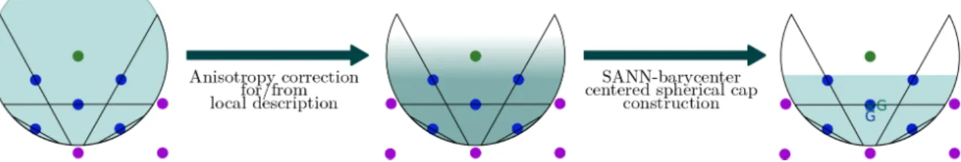
The basic idea of the ASANN algorithm is that some directions are more relevant for coordination than others. Therefore, instead of requiring the neighbors to fill up the whole field of view, ASANN only requires to fill up the relevant neighboring region of space (see Figure 4).
An estimator of the first order local anisotropy is obtained based on the barycentre. Specifically, we define the SANN-based barycentre ~G(m)i as the position barycentre over all SANN-coordinated neighbors of i, weighted by their SANN-based solid angle Ωi,j (with respect to i). A similar solid-angle based neighbors weighting has been proposed in the
FIG. 4: Illustration of the SANN coordination number overestimation, and founding idea of the ASANN algorithm: tackle local anisotropy by focusing on relevant regions for coordination. This leads to the consideration of a coordination spherical cap instead of a sphere. The chosen spherical cap reproduces the local anisotropy, through our first order local anisotropy estimator (using a SANN-based barycentre with solid-angle weighting).
context of the Voronoi tessalationfor its canonicity.11 Mathematically, this can be written:
~ G(m)i = m P j=1 Ωi,j~ri,j m P j=1 Ωi,j (4)
This SANN-based barycentre is in agreement with the properties expected for retrieving the first order local anisotropy. Indeed, it identifies a global privileged direction in the distribution of coordinating neighbors and, more importantly, it provides with a quantitative estimation of the first order local anisotropy magnitude α(m)i defined by:
α(m)i = || ~G (m) i ||
R(m)i (5)
Instead of considering a coordination sphere, the ASANN algorithm uses a coordination spherical cap C which focuses on the locally relevant region of space for coordination. Ci is the spherical cap centered on i having the same anisotropic properties as the neighboring particles through our first order local anisotropy estimator. This is achieved by setting the radius RCi = R
(m)
i and requiring that its barycentre ~GCi is confounded with the SANN-based
barycentre ~G(m)i : Ci is centred on i RCi = R (m) i ~ GCi = ~G (m) i (6)
The solid angle ΩCi associated with this spherical cap (with respect to i) can be written
as:
ΩCi = 4π(1 − γCi) (7)
where γCi ∈ [0, 1[ corresponds to the angular correction coefficient, which only depends on
the first order local anisotropy magnitude α(m)i (see section S1 in the SI for a derivation):
γCi =
α(m)i + q
α(m)i 2+ 3αi(m)
3 (8)
Therefore, instead of filling up the whole field of view ( m P
j=1
Ωi,j = 4π), ASANN neighbors only cover the spherical cap. This leads to the fundamental equation of ASANN:
m0 X j=1 Ω0i,j = m0 X j=1 2π 1 − ri,j R0(mi 0) ! = ΩCi = 4π(1 − γCi) (9)
where the ASANN coordination number m0and the coordination cap radius R0(mi 0)are defined by extending the SANN coordination radius definition to include the angular correction coefficient γCi: R0(mi 0) = m0 P j=1 ri,j m0− 2 × (1 − γ Ci) < ri,m0+1 (10)
Note that for isotropic distributions (γCi = 0), Eq. 10 goes back to Eq. 3, which means that
SANN and ASANN coincide for this case.
Using the inequality of Eq. 10, the ASANN coordination number m0 can be easily com-puted by iteratively computing R0(mi 0), starting with m0 = b2(1 − γCi)c + 1, and increasing
m0 until the inequality is respected.
In principle, this angular correction could be computed self-consistently, i.e., the angular correction term is recomputed at each iteration along with the ASANN coordination radius. This self-consistency breaks the analytic, direct link between the fundamental equation (Eq. 9) and the coordination radius definition (Eq. 10). Therefore, we only explore the “per-turbative” angular correction, where the SANN-based barycentre ~G(m)i and the associated angular correction term γCi are computed only once, using the SANN-based coordination
radius and coordinating neighbors. Then, the iterative ASANN algorithm (Eq. 10) is per-formed with a fixed γCi. As demonstrated in the supporting information, this algorithm
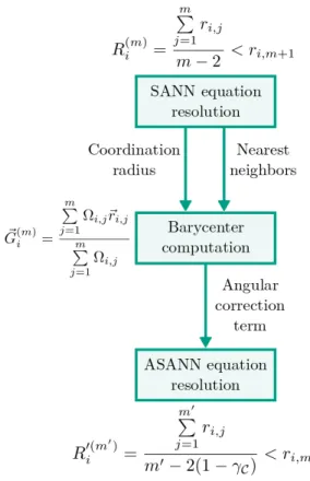
FIG. 5: Schematic representation of the ASANN workflow: Based on the SANN coordination sphere, the barycenter and the corresponding angular correction is computed,
leading to the ASANN coordination spherical cap.
which also provides information regarding the computational cost of ASANN compared to SANN: Essentially, there is a factor of two between them, since the iterations have to be performed twice. Knowing that ASANN coordination number is lower or equal to the one from SANN (see SI for a proof), there are, in general, less ASANN than SANN iterations.
Based on general properties of ASANN, partially inherited from SANN, we show the expected applicability domain of the two algorithms in Figure 6. The first major limitation is related to low coordination numbers (e.g., four) in combination with isotropic distributions (e.g., a tetrahedron). In this case, the coordination radius R(4)i of Eq. 3 is twice the distance between atom i and its nearest neighbors j. If there are atoms closer than 2rij, the inequality is not satisfied and the coordination shell is expanded to include next nearest neighbors. This is the case for most organic molecules (see Figs. S2-S5 and the associated discussion), but
also in ionic compounds where small cations are located in tetrahedral sites as shown in the SI (Tables S4 to S15), where we have analyzed a variety of salts, oxides and perovskites. The particularity of these systems is most clearly seen for the case of a graphene sheet (Fig. S5): the barycenter of neighboring atoms is confounded with the central atom, so there is no first order anisotropy and ASANN is equivalent to SANN. There are three nearest neighbor atoms at a distance rC−C and the next nearest neighbors are already at
√
3rC−C, again due to the directional bonding, but which is well below the R(3)i = 3rC−C (Eq. 3 for the perfect symmetry of this system). If there would not be an anisotropic preference due to bond formation characteristic for an sp2 carbon atom, there would also be “space” for at least two more particles one above and one below the plane within such a coordination sphere. But this is not the case and, therefore, for geometrical reasons, ASANN significantly overestimates the conventional coordination number of 3, by adding the 6 next nearest neighbors, reaching a CNASANN=9 for carbon in graphene. The same geometrical reasons and deviations from homogeneous distributions apply to the ionic compounds referred to above. Since ASANN is built on a first order anisotropy, the application to nanopores or slits is also at the border of its applicability: if the SANN coordination sphere spans two surfaces, the first order anisotropy vanishes and ASANN does not improve upon SANN. Higher order anisotropy corrections might correct SANN in this situation as well as for the isotropic, low-coordination environments mentioned above. Second, density fluctuations are problematic for the scale free algorithms. Therefore, cross-checks with the coordination radii are required for biphasic systems and the liquid-gas interface. As we will show by numerical results below, ASANN extends, however, the applicability of SANN to (inhomogeneous) solutions, the solid-liquid interface and rough surfaces including nano-particles.
The time complexity of (A)SANN is in the worst-case O(nk) for pre-treated input, where n is the number of particles, and k is the maximum coordination number. In fact, the most time consuming step is due to the input pre-processing, required for both SANN and ASANN algorithms. This pre-processing comprises the computation of pair-wise distances (and vectors for ASANN) in O(n2), and sorting those distances in O(n2log(n)). It is, there-fore, this step that is also responsible for the space complexity of (A)SANN in O(n2). In practice, this pre-processing quickly becomes the computational bottleneck for large sys-tems. As a consequence, particular care was taken for optimizing these steps in our Python 3 implementation, heavily relying on the Numpy library27,28. We thus combine low-level
FIG. 6: Venn diagram depicting the applicability domains of both SANN and ASANN. By design, ASANN extends the applicability domain of SANN to systems presenting local
anisotropy.
language performance for large systems, with convenient Python 3 syntax and modularity. As an example, the computation of the Cs coordination numbers in a 742 atom system (vide infra), took around 0.14 seconds and the computation of all coordination numbers in a 2942 atom system took about 2 seconds (93% is spent on input pre-processing) on a personal laptop (Core i5-6300HQ CPU).
III. COMPUTATIONAL DETAILS
The presented algorithms have been implemented using Python329 and are available in the supporting information and also on the webpage of the authors. The implementation relies on the Numpy library27,28whenever possible and ASE12for reading common coordinate formats. A particular effort was made to provide with extensively commented code, including documentation and illustrative examples.
Figures have been generated with a custom ASE12 fork to visualize the coordination numbers.
All DFT computations are performed using VASP30,31. The PBE exchange-correlation functional32 was applied and a 400 eV energy cut-off was chosen for the plane-wave basis set. The PAW pseudo-potentials were used for describing the electron–ion interactions.33,34
Some of the optimized metallic surfaces and metal clusters have been previously published by our group.35–37 The graphite electrode was set up as follows: A symmetric six layer p(2×2) graphite slab has been built based on the optimized bulk geometry using the PBE-dDsC38 level of theory. A 9 × 9 × 1 Monkhorst-Pack K-point grid was used to integrate the Brillouin zone. To assess the charge distribution at negative potentials, the number of electrons was varied and the linearized Poisson-Boltzmann equation was utilized to neutralize the unit cell as implemented in the VASPsol package.39,40 Similarly to our previous study on electroreduction in aprotic medium,41 the isodensity value defining the cavity has been lowered to 5 10−4 e/˚A3. In the case of graphite, this value ensures an absence of implicit solvent between the dispersion bound graphene layers.
The potential of zero charge of graphite is, according to our setup, -0.2 V vs SHE, which compares reasonably well with experiments (0.1 to 0.3 V depending on the nature of the carbon electrode42–44) considering the idealized morphology of our electrode and the expected systematic error due to the simplified electrolyte model as discussed in the context of the potential dependent adsorption of pyridine on a gold single crystal surface45. A negative charge of -0.25 electrons in the unit cell (-0.125 electrons per surface) led to a potential drop of 2.4 V compared to the potential of zero charge and thus corresponds to a significant negative polarization. Based on the DFT computations, the unit cell was replicated four times in each in-plane direction, resulting in 128 carbon atoms per layer and a total charge of 4 e-. Following a setup very similar to ref 46, the Lennard-Jones (LJ) parameters for graphite are taken from UFF.47 The initial solvent distribution is obtained from the predefined TIP3P48 box with about 35 ˚A of water surrounding the system, resulting in a box of 716 water molecules. To simulate a 1 M electrolyte, 15 Na+ (or Cs+) and 11 Cl− ions, described by their standard AMBER force field parameters, are added using tleap of the AmberTools. MM computations are performed with NAMD 2.949 for 5 ns (time step of 2 fs), applying a Langevin thermostat (300 K) with a damping coefficient of 1 ps-1. The Langevin barostat (1 bar) is applied with a piston period of 100 fs and a decay of 150 fs.
IV. RESULTS AND DISCUSSION
A. Metallic surfaces
As a first test, we apply ASANN to various metallic surfaces. The selection of surfaces is intended to span a wide range of typical cases to assess the applicability domain of SANN and ASANN.
For face centered cubic (fcc) metallic surfaces, the metal-metal contact distance in the bulk is a reliable measure for identifying nearest neighbors. Reassuringly, closed packed, flat surfaces are well described by SANN and ASANN, giving identical results that are in perfect agreement with cutoff based methods (see SI). In other words, flat surfaces are not anisotropic enough to induce an expansion of the SANN coordination sphere to the next nearest neighbors.
An increased local anisotropy can be obtained for nano-rods. The large rod, constructed from the corresponding bulk without any geometry optimization (Figure 7), is still well and identically described by SANN and ASANN.
However, stepped surfaces (see Figures 8 and 9) are more challenging for SANN, while ASANN consistently retrieves the cutoff based coordination number. In particular, SANN is very sensitive to small local surface induced contractions, while ASANN is more robust, avoiding coordination number overestimations seen in Figure 9 for SANN.
To simulate low-coordinated atoms,9 add-atoms have also been analyzed. Based on visual inspection (and confirmed by cutoff based methods), the square of addatoms on a (100) sur-face is characterized by two nearest neighbors from the square (the third is not “touching”, i.e., it is a next-nearest neighbor) and four from the (100) plane below, yielding a coordina-tion number of six. Similarly, an addatom of the triangle on a (111) surface possesses two nearest neighbors from the triangle and three from the supporting (111) plane, resulting in a coordination number of five. Recalling that the flat (100) surface of fcc closed packed metals has a coordination number of 8 for its surface atoms, the CNSANN=8 for surface addatoms reveal a clear overestimation (see Figures 10 and 11), qualitatively failing to identify the low-coordination environment. This contrasts with CNASANN that is in full agreement with visual inspection and cuttoff based methods.
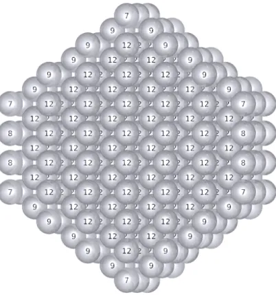
FIG. 7: Transversal cut of a periodic nano-rod of an fcc metal, with superimposed coordination numbers. SANN and ASANN coordination numbers are identical.
FIG. 8: Side view of a stepped gold surface (664), with superimposed coordination numbers. SANN and ASANN coordination numbers are identical.
(a) SANN (b) ASANN
FIG. 9: Side view of a stepped gold surface (644), with superimposed SANN (a) and ASANN (b) coordination numbers.
(a) ASANN algorithm (b) SANN algorithm
FIG. 10: Representation of a p(3×3) Cu(100) surface with a square of 4 Cu addatoms. Coordination numbers from SANN (a) and ASANN (b) are superimposed.
nanoparticle (see Figure 12). As can be seen, the particle features atoms that clearly form tips and, therefore, we expect low CNs for them. However, just like for the addatoms on the planar surfaces, SANN fails to correctly identify these low-coordinated atoms. For these highly aniostropic distributions, the SANN coordination radius has to expand significantly to
(a) ASANN algorithm (b) SANN algorithm
FIG. 11: Representation of a p(3×3) Cu(111) surface with a triangle of 3 Cu addatoms. Coordination numbers from SANN (a) and ASANN (b) are superimposed.
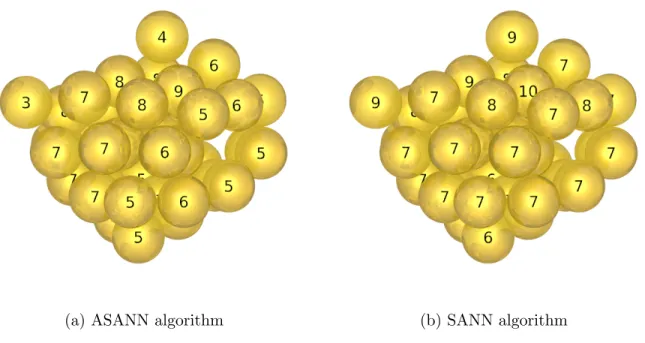
(a) ASANN algorithm (b) SANN algorithm
FIG. 12: Low energy, amorphous Au38nanoparticle. Coordination numbers from SANN (a) and ASANN (b) are superimposed. SANN overestimation is particularly visible at the tips.
reach the entire 4π for the sum of solid angles. In contrast, ASANN exploits the aniosotropy of the SANN coordination sphere to construct a spherical cap and, therefore, succeeds in identifying intuitive nearest neighbors in all cases.
As a rule of thumb, we empirically found that SANN rarely finds coordination num-bers below 7 in these systems, illustrating the surface-related overestimation reported earlier.23 ASANN, however, performs very well in all tested systems, correctly identify-ing low-coordination environments. As shown in the supportidentify-ing information, this robust, parameter-free performance is also transmitted to generalized coordination numbers9 of various surfaces, dispensing with the need to define a characteristic distance or manual counting.
B. Coordination numbers at charged interfaces
The interaction of cations with negatively charged electrodes is of growing interest in the electro-reduction of CO and CO2.50–52In a different context, electrolyte solutions at charged silica interfaces are widely studied to understand the behavior of confined electrolytes.53 Finally, the advent of carbon based supercapacitors54,55has spurred simulations of electrolyte solutions at charged carbon interfaces.56,57Such simulations are also of particular interest to understand the intercalation mechanism of alkali metal ions into graphitic surfaces.58 Here, we consider a simple model system: aqueous salt solutions in contact with a perfect graphite electrode. On the one hand, the experimental capacitance of a graphitic electrode is not strongly dependent on the alkali cation in the electrolyte,59 which might suggest that the double layer structure is similar for all alkali metal cations. On the other hand, Cs+ ions are, in contrast to Na+ ions, known to be soft and large, implying a low charge density at their surface. As a consequence, Cs+ions are expected to partially loose their solvation shell to approach the negatively charged electrode surface more closely, which increases both the VdW interactions and the Coulomb attraction.
We probe the difference between Cs+ and Na+ based on classical molecular dynamics simulations of a graphite carbon electrode at a potential of about -2.5 V (see Computational Details) in ∼1 M aqueous CsCl and NaCl solutions. To analyze the double layer, we inves-tigate the existence of a link between coordination number of ions in water (determined by ASANN, SANN and a g(r) based cut-off algorithm) and their adsorption state.
Figure 13 displays the structuring of the electrolyte at the electrode surface. As com-monly observed60, for both electrolyte solutions the distribution curve of the excess cation density presents two well-defined peaks, corresponding to two distinct layers of preferred
FIG. 13: Ionic density of ∼1 M CsCl (top pannel) and NaCl (bottom pannel) aqueous solutions near a graphite anode (−2.5 V vs SHE). The excess counter-ions (compared with
the co-ions, equivalent here to the charge density) and the co-ions density are represented for both systems. Three distinct zones are identified, corresponding to different adsorption/trapping states for the counter-ions. The average ASANN coordination number
for the counter-ions (with water molecules and co-ions) is superimposed for each zone.
presence near the anode. The strong first cation excess peak is followed by a nearly charge compensated zone before a second, although lower, cation excess peak occurs which then decays to zero towards the bulk solution. Besides, the anion (Cl−) distribution is barely structured and independent on the nature of the cation. The details of the charge-excess profiles are quite different: Cs+ excess density has the first peak at about 3.5 ˚A, while the corresponding one for Na+ is at 4.8 ˚A. This difference indicates that Cs+ can indeed ap-proach the electrode more closely. The second peak is, accordingly, shifted from 6 ˚A to 7.5 ˚
A when going from caesium to sodium.
Table I and II report the ASANN and SANN coordination numbers of Cs+ and Na+, respectively. For reference purposes, the radial distribution function of the O-Cs+ was analysed and a first coordination sphere radius cutoff of 4.0 ˚A was identified. From this radius, cutoff-based coordination numbers have been computed. All three algorithms agree that on average at least one water molecule is lost when Cs+ is located in the first layer,
Average coordination numbers of Cs+ ions
Method Desolvated trapping layer h < 4.7 ˚A
Solvated trapping layer 4.7 < h < 7 ˚A Bulk-like layer h > 7 ˚A ASANN 7.4 (1.1) 9.6 (1.2) 9.4 (1.2) SANN 9.1 (1.1) 10.6 (1.2) 10.5 (1.2) fixed cutoff 7.1 (1.1) 9.2 (1.3) 9.0 (1.3)
TABLE I: Comparison of average Cs+ ions coordination numbers determined by ASANN, SANN and a fixed cutoff (4.0 ˚A) for each defined region. The data is displayed in the form:
mean (standard deviation).
while the second layer is indistinguishable from the bulk solution in terms of the coordination numbers. This can be rationalized based on Van der Waals (VdW) radii: a fully solvated Cs ion cannot approach the graphitic electrode closer than roughly 7 ˚A (rC + rCs+ + 3 ˚A,
where 3 ˚A is a rough estimate for the size of a water molecule).
For Na+ ions, however, the coordination numbers are the same in the two excess regions as in the bulk, despite the qualitative similarity between the two cation excess profiles. Even the nearest Na+ layer (∼ 4.8 ˚A) is not close enough to the surface to induce a partial desolvation (see Table II). In other words, in contrast to Cs+, the solvation shell of Na+ is strong and stable across the double layer and the three methods agree on an approximate average coordination number of six, indicating minor fluctuations and a rather isotropic distribution, in agreement with spectroscopic data.6
To quantitatively determine if ASANN provides with “good” coordination numbers, we assess their ability to discriminate between “close” and “bulk” Cs ions. Specifically, we want to quantify if CNASANN is statistically lower (i.e., below CNthresh) at the interface than in the bulk. For the sake of comparison, we apply the same analysis also to SANN and to the cutoff based algorithm.
To have a quantifiable measure whether or not CNASANNis lower at the interface than in the bulk, we explore the relation between closeness and loss of coordination via a Receiver Operating Characteristic (ROC) curve analysis. The ROC curve is one of the most rigorous and well-established tools to evaluate the discriminating power for a binary classifier (here
Average coordination numbers of Na+ ions
Method First trapping layer h < 6.5 ˚A
Second trapping layer 6.5 < h < 9 ˚A Bulk-like layer h > 9 ˚A ASANN 6.1 (0.6) 6.1 (0.6) 6.1 (0.5) SANN 6.5 (0.7) 6.6 (0.8) 6.5 (0.8) fixed-cutoff 5.8 (0.5) 5.8 (0.5) 5.8 (0.5)
TABLE II: Comparison of average Na+ ions coordination numbers determined by ASANN, SANN and a fixed cutoff (3.2 ˚A) for each defined region. The data is displayed in the form:
mean (standard deviation).
close/not close) depending on a threshold value (here CNASANN).61,62 The ROC curve of a class of binary classifiers is constructed by plotting the True Positive Rate (TPR) against the False Positive Rate (FPR) computed on a data set, for different threshold values.
Here, the TPR is the ratio of CNi <CNthresh for the i Cs ions “close” to the electrode to the number of Cs ions “close” to the electrode overall, while the False Positive Rate is the ratio of CNi <CN
thresh for Cs ions not “close” to the electrode to the number of Cs ions not “close” to the electrode overall. The threshold value can be varied between the minimum and maximum observed with a given algorithm. Here, we define “close” as the Cs – surface distance ≤ 4.7 ˚A.
Such an analysis is reported on Figure 14. Let us first look at the ASANN results to explain how to read a ROC curve. Since the CNs are reasonable descriptors, for low CNthresh (e.g., 7), only “close” Cs ions are identified (FPR=0%), but not all of them (TPR≈20%), as shown in Table S16a. Similarly, at high CN (e.g., 10), the TPR reaches ≈100%, i.e., all “close” Cs ions have CNs below this value, but about 50% (FPR) of the ions not close to the surface have CNs below this value. Hence, increasing the threshold further does not change the TPR, but the FPR reaches 100%.
A major ROC curve analysis is performed through the Area Under the Curve (AUC), as it provides an aggregate measure of classification performance63. In this particular example, the AUC is associated with the probability that a random interfacial Cs ion has a lower coordination number than a random bulk Cs ion.
FIG. 14: ROC curve for classifying Cs ions for being “close” to the carbon anode based on the coordination number being below a given threshold. When moving from TPR=20% to TPR=55% with ASANN (blue curve), CNthresh is increased from 7 to 8 (see Table S16a in the SI for the raw data). This exploits the geometrical constraint responsible for a partial
desolvation when close enough to the surface. The distance criterium for being close enough to the surface is chosen to be 4.7 ˚A, since it corresponds to the empirical frontier between the partially desolvated adsorption zone and the fully solvated adsorption zone for
Cs ions near the graphite anode (see Fig. 13).
With an AUC of 0.90, we find a strong correlation between CNASANN and the proximity of Cs+ and the surface. This finding is coherent with ASANN providing reasonable coor-dination numbers in this system. The same analysis performed with SANN only yields an AUC of 0.81. The cutoff-based algorithm yields an AUC of 0.86, outperforming SANN, but not reaching the performance of ASANN. This is rather remarkable, given that the cutoff algorithm is tuned to the system by analyzing the radial distribution function, while ASANN does not know anything about the specificities of the system. On a physical level, the ma-jor difference between the cutoff algorithm and ASANN is that the ASANN coordination sphere adapts itself to the local environment, while the cutoff does not. This means that the
cutoff based CNs are more sensitive to thermal fluctuations. Indeed, we found cutoff-based coordination numbers to be slightly noisier (≈ +8%) than their ASANN/SANN counter-parts within each region of the studied system (see Table I), rationalizing the poorer AUC performance.
From this comparison it can be concluded that fixed-cutoff based algorithms are some-what challenged when dealing with liquids, while SANN is not suitable for interfaces. In contrast, ASANN combines the best features of these algorithms and performs well. There-fore, ASANN is most relevant for describing solid/liquid interfaces.
C. Application to Au NP energy fitting
Exploring the energy landscape of alloy nano-particles from first principles is computa-tionally very expensive. Therefore, cheap energy evaluations based on simplified Hamilto-nians are often applied.64–66. Furthermore, if the model Hamiltonian captures the essential physics, it can also be used to gain insight into the driving force of the alloy formation. Inspired from cluster expansions, we here test the use of a simple model Hamiltonian Hm for bimetallic materials. Hm depends only on the number of atoms of each element and the number of bonds between each possible elements pairs:
Hm = X χ ΓχNχ+ X χ,χ0≥χ Γχ,χ0Nχ,χ0 (11)
In other words, it is a two-body model Hamiltonian. For alloys of elements with quite different atomic radii, the alloy nano-particles are not necessarily very regular and selecting characteristic distances is not straight forward. Therefore, an automatic, parameter free algorithm to identify bonds is particularly beneficial for these systems. In the following, we apply this simplified model to bimetallic Au-Cu materials, where Hm becomes
Hm= ΓAuNAu+ ΓCuNCu+ ΓAu,AuNAu,Au+ ΓAu,CuNAu,Cu+ ΓCu,CuNCu,Cu = Γ · N
(12)
with Γ the set of parameters to fit. N is constructed by enumeration of atoms and bonds of each type. The automatic bond enumeration was performed using ASANN and SANN for comparison purposes. In order to have consistent bond description, a bond between atoms A and B is only counted if and only if B is found as nearest neighbor of A and reciprocally.
FIG. 15: Parity plot for the total energy predicted by a 2-body model Hamiltonian fitted using the SANN vs. ASANN coordination algorithm. The whole set of 27 nanoparticles + 6 Bulk structures was used as training set, and the test set was composed of the 27 Au-Cu
bimetallic nanoparticles only for graphical considerations.
Such filtering is particularly beneficial to SANN, where buried atoms are mostly spared from coordination overestimation. Hence, the bidirectional bond definition improves the soundness of bonds between bulk and surface atoms.
For fitting the model Hamiltonian, we use a structurally diverse set of 27 Au-Cu bimetallic nanoparticles composed of 38 atoms with various compositions and morphologies and 6 Au-Cu bulk structured alloys with various Au-Au-Cu ratios. The coordinates are provided in the supplementary information.
When fitting only the nanoparticle set, the algorithms lead to model Hamiltonians with mean absolute deviation (MAD) of 0.8 eV for ASANN and 0.7 eV for SANN, see Figure S1. In other words, both approaches are very similar, with SANN performing slightly better than ASANN. However, the ASANN-derived parameters are found to be more robust than their SANN-based counterparts when adding the bulk structured alloys to the training
set (i.e. diversifying the training set). The fitted parameters are not only slightly less impacted (see Tables S1 and S2 in the SI), but the overall model performance is better with ASANN-based bonds (MAD near 1.5 eV for ASANN, versus 1.8 eV for SANN). This is especially true when using only the nanoparticles as test set. The predicted energy for the nanoparticles with respect to the DFT reference energies yields a coefficient of determination R2 = 0.72 and R2 = 0.59 with ASANN and SANN based 2-body patterns, respectively (see Figure 15). Similarly, the pure bulks are better described by ASANN (MAD=0.37 eV), than SANN (MAD=0.60 eV). Hence, the better performance of SANN for exclusively fitting the nanoparticles set can be traced back to error cancellation between coordination number overestimation and missing higher-order many-body terms at the surface. In summary, we conclude that ASANN provides a balanced and physical sound description between bulk and surface-rich nanoparticles. Therefore, ASANN can also be applied to alloys of elements with quite different atomic radii. Similarly, ASANN could be used to provide a simple estimation of the surface of nanoparticles, by considering the union (or surface sum) of the planar edge of each coordination cap. A more rigorous approach using ASANN to define the surface of nanoparticles would be through the definition of a locally adaptative coordination radius, defining the local coarseness of the surface.
V. CONCLUSION
In this work we have extended the solid-angle based nearest-neighbor (SANN) algorithm to account for the local anisotropy, defining the anisotropically corrected solid-angle based nearest-neighbor (ASANN) method. ASANN allows to efficiently compute parameter-free coordination numbers and significantly improves over SANN at interfaces, where the coor-dination environment is highly anisotropic, such as nano-particles and partially desolvated ions at solid/liquid interfaces, where SANN leads to overestimations of the coordination number. In all situations tested, the ASANN coordination numbers are either identical or physically more sound than the ones provided by SANN and on par with system-specific, cut-off based coordination numbers. Therefore, ASANN provides a robust method to compute coordination numbers for describing alloy nano-particles, extended surfaces and (electrified) solid/liquid interfaces.
ACKNOWLEDGMENTS
We thank Paul Clabaut, Mathilde Iachella, David Loffreda and Kamila Kazmierczak for providing us the geometries of nanorods and nanoparticles, bulk alloys and cobalt sur-faces, respectively. The authors thank the SYSPROD project and AXELERA Pˆole de Comp´etitivit´e for financial support (PSMN Data Center).
VI. SUPPLEMENTARY MATERIAL
Additional Theorems, Figures and Tables are available in the supplementary material.
REFERENCES
1A. E. Reed, L. A. Curtiss, and F. Weinhold, Chem. Rev. 88, 899 (1988). 2H. Elgabarty, R. Z. Khaliullin, and T. D. Kuhne, Nat. Commun. 6 (2015).
3L. Pecher, S. Laref, M. Raupach, and R. Tonner, Angew. Chem., Int. Ed. 56, 15150 (2017).
4R. Staub, M. Iannuzzi, R. Z. Khaliullin, and S. N. Steinmann, Journal of Chemical Theory and Computation 15, 265 (2019).
5J. Marcalo and A. P. De Matos, Polyhedron 8, 2431 (1989). 6J. Mahler and I. Persson, Inorg. Chem. 51, 425 (2012).
7S. Varma and S. B. Rempe, Biophysical Chemistry 124, 192 (2006).
8L. M. Falicov and G. A. Somorjai, Proceedings of the National Academy of Sciences 82, 2207 (1985).
9F. Calle-Vallejo, J. I. Mart´ınez, J. M. Garc´ıa-Lastra, P. Sautet, and D. Loffreda, Ange-wandte Chemie International Edition 53, 8316 (2014).
10F. C. Frank and J. S. Kasper, Acta Cryst 11, 184 (1958).
11M. O’Keeffe, Acta Crystallogr A Cryst Phys Diffr Theor Gen Crystallogr 35, 772 (1979). 12A. H. Larsen, J. J. Mortensen, J. Blomqvist, I. E. Castelli, R. Christensen, M. Duak, J. Friis, M. N. Groves, B. Hammer, C. Hargus, E. D. Hermes, P. C. Jennings, P. B. Jensen, J. Kermode, J. R. Kitchin, E. L. Kolsbjerg, J. Kubal, K. Kaasbjerg, S. Lysgaard, J. B. Maronsson, T. Maxson, T. Olsen, L. Pastewka, A. Peterson, C. Rostgaard, J. Schitz,
O. Schtt, M. Strange, K. S. Thygesen, T. Vegge, L. Vilhelmsen, M. Walter, Z. Zeng, and K. W. Jacobsen, Journal of Physics: Condensed Matter 29, 273002 (2017).
13B. Cordero, V. Gmez, A. E. Platero-Prats, M. Revs, J. Echeverra, E. Cremades, F. Bar-ragn, and S. Alvarez, Dalton Trans. , 2832 (2008).
14C. A. Coulson and G. S. Rushbrooke, Phys. Rev. 56, 1216 (1939).
15J. G. Kirkwood and E. M. Boggs, The Journal of Chemical Physics 10, 394 (1942). 16W. Brostow, Chemical Physics Letters 49, 285 (1977).
17P. G. Mikolaj and C. J. Pings, Physics and Chemistry of Liquids 1, 93 (1968). 18J. D. Bernal, Trans. Faraday Soc. 33, 27 (1937).
19A. Rahman, The Journal of Chemical Physics 45, 2585 (1966).
20J. L. Finney and J. D. Bernal, Proceedings of the Royal Society of London. A. Mathemat-ical and PhysMathemat-ical Sciences 319, 479 (1970).
21J. A. van Meel, L. Filion, C. Valeriani, and D. Frenkel, The Journal of Chemical Physics 136, 234107 (2012).
22H. Ledoux, in 4th International Symposium on Voronoi Diagrams in Science and Engi-neering (ISVD 2007) (2007) pp. 117–129.
23J. Higham and R. H. Henchman, The Journal of Chemical Physics 145, 084108 (2016). 24J. K. Noel, P. C. Whitford, and J. N. Onuchic, The Journal of Physical Chemistry B 116,
8692 (2012).
25R. Taylor, CrystEngComm 16, 6852 (2014).
26R. Collins, Proceedings of the Physical Society 86, 199 (1965).
27T. E. Oliphant, Guide to NumPy, 2nd ed. (CreateSpace Independent Publishing Platform, USA, 2015).
28S. v. d. Walt, S. C. Colbert, and G. Varoquaux, Computing in Science & Engineering 13, 22 (2011).
29G. Van Rossum and F. L. Drake, Python 3 Reference Manual (CreateSpace, Paramount, CA, 2009).
30G. Kresse and J. Hafner, Phys Rev B 47, 558 (1993).
31G. Kresse and J. Furthmuller, Phys Rev B 54, 11169 (1996).
32J. P. Perdew, K. Burke, and M. Ernzerhof, Phys Rev Lett 77, 3865 (1996). 33P. E. Blochl, Phys Rev B 50, 17953 (1994).
35A. Viola, J. Peron, K. Kazmierczak, M. Giraud, C. Michel, L. Sicard, N. Perret, P. Beau-nier, M. Sicard, M. Besson, and J.-Y. Piquemal, Catal. Sci. Technol. 8, 562 (2018). 36M. Dhifallah, M. Iachella, A. Dhouib, F. Di Renzo, D. Loffreda, and H. Guesmi, J. Phys.
Chem. C 123, 4892 (2019).
37R. V. Mom, S. T. A. G. Melissen, P. Sautet, J. W. M. Frenken, S. N. Steinmann, and I. M. N. Groot, J. Phys. Chem. C 123, 12382 (2019).
38S. N. Steinmann and C. Corminboeuf, J Chem Theory Comput 7, 3567 (2011).
39K. Mathew, R. Sundararaman, K. Letchworth-Weaver, T. A. Arias, and R. G. Hennig, J Chem Phys 140, 084106 (2014).
40K. Mathew, V. S. C. Kolluru, S. Mula, S. N. Steinmann, and R. G. Hennig, J. Phys. Chem. , DOI: 10.1063/1.5132354 (2019).
41S. N. Steinmann, C. Michel, R. Schwiedernoch, and P. Sautet, Phys. Chem. Chem. Phys. 17, 13949 (2015).
42B. Kastening and S. Spinzig, Journal of Electroanalytical Chemistry and Interfacial Elec-trochemistry 214, 295 (1986).
43H. R. Zebardast, S. Rogak, and E. Asselin, Journal of Electroanalytical Chemistry 724, 36 (2014).
44J. Poon, C. Batchelor-McAuley, K. Tschulik, and R. G. Compton, Chemical Science (2015).
45S. N. Steinmann and P. Sautet, J. Phys. Chem. C 120, 5619 (2016).
46S. N. Steinmann, P. Sautet, and C. Michel, Phys. Chem. Chem. Phys. 18, 31850 (2016). 47A. K. Rappe, C. J. Casewit, K. S. Colwell, W. A. Goddard, and W. M. Skiff, J Am Chem
Soc 114, 10024 (1992).
48W. L. Jorgensen, J. Chandrasekhar, J. D. Madura, R. W. Impey, and M. L. Klein, J Chem Phys 79, 926 (1983).
49J. C. Phillips, R. Braun, W. Wang, J. Gumbart, E. Tajkhorshid, E. Villa, C. Chipot, R. D. Skeel, L. Kal´e, and K. Schulten, J Comput Chem 26, 1781 (2005).
50J. Resasco, L. D. Chen, E. Clark, C. Tsai, C. Hahn, T. F. Jaramillo, K. Chan, and A. T. Bell, J. Am. Chem. Soc. 139, 11277 (2017).
51E. P´erez-Gallent, G. Marcandalli, M. C. Figueiredo, F. Calle-Vallejo, and M. T. M. Koper, J. Am. Chem. Soc. 139, 16412 (2017).
52S. Ringe, E. L. Clark, J. Resasco, A. Walton, B. Seger, A. T. Bell, and K. Chan, Energy Environ. Sci. , 10.1039.C9EE01341E (2019).
53T. A. Ho, D. Argyris, D. R. Cole, and A. Striolo, Langmuir 28, 1256 (2012).
54S. Bose, T. Kuila, A. K. Mishra, R. Rajasekar, N. H. Kim, and J. H. Lee, J. Mater. Chem. 22, 767 (2011).
55X. Chen, R. Paul, and L. Dai, Natl Sci Rev 4, 453 (2017).
56C. Merlet, C. P´ean, B. Rotenberg, P. A. Madden, P. Simon, and M. Salanne, J. Phys. Chem. Lett. 4, 264 (2013).
57A. C. Forse, C. Merlet, J. M. Griffin, and C. P. Grey, J. Am. Chem. Soc. 138, 5731 (2016). 58M. Petrovi´c, I. ˇSrut Raki´c, S. Runte, C. Busse, J. T. Sadowski, P. Lazi´c, I. Pletikosi´c, Z.-H. Pan, M. Milun, P. Pervan, N. Atodiresei, R. Brako, D. ˇSokˇcevi´c, T. Valla, T. Michely, and M. Kralj, Nat Commun 4, 2772 (2013).
59D. Golub, A. Soffer, and Y. Oren, Journal of Electroanalytical Chemistry and Interfacial Electrochemistry 260, 383 (1989).
60D. A. Welch, B. L. Mehdi, H. J. Hatchell, R. Faller, J. E. Evans, and N. D. Browning, Advanced Structural and Chemical Imaging 1, 1 (2015).
61K. A. Spackman, in Proceedings of the Sixth International Workshop on Machine Learning, edited by A. M. Segre (Morgan Kaufmann, San Francisco (CA), 1989) pp. 160–163. 62T. Fawcett, Pattern Recognition Letters ROC Analysis in Pattern Recognition, 27, 861
(2006).
63C. Ferri, J. Hern´andez-Orallo, and P. A. Flach, in Proceedings of the 28th International Conference on Machine Learning (ICML-11) (2011) pp. 657–664.
64W. Chen, D. Schmidt, W. F. Schneider, and C. Wolverton, J. Phys. Chem. C 115, 17915 (2011).
65B. Zhu, J. Creuze, C. Mottet, B. Legrand, and H. Guesmi, J. Phys. Chem. C 120, 350 (2016).
66E. Vignola, S. N. Steinmann, K. Le Mapihan, B. D. Vandegehuchte, D. Curulla, and P. Sautet, J. Phys. Chem. C 122, 15456 (2018).