HAL Id: tel-00694201
https://tel.archives-ouvertes.fr/tel-00694201
Submitted on 4 May 2012
HAL is a multi-disciplinary open access
archive for the deposit and dissemination of sci-entific research documents, whether they are
pub-L’archive ouverte pluridisciplinaire HAL, est destinée au dépôt et à la diffusion de documents scientifiques de niveau recherche, publiés ou non,
Viana maps and limit distributions of sums of point
measures
Daniel Schnellmann
To cite this version:
Daniel Schnellmann. Viana maps and limit distributions of sums of point measures. Dynamical Systems [math.DS]. Royal Institute of Technology (KTH), 2009. English. �tel-00694201�
Viana maps and limit distributions of
sums of point measures
DANIEL SCHNELLMANN
Doctoral Thesis
Stockholm, Sweden 2009
TRITA-MAT-09-MA-14
ISSN 1401-2278
ISRN KTH/MAT/DA 09/10-SE
ISBN 978-91-7415-521-1
KTH Matematik
SE-100 44 Stockholm
SWEDEN
Akademisk avhandling som med tillstånd av Kungl Tekniska högskolan
framlägges till offentlig granskning för avläggande av teknologie
dok-torsexamen i matematik torsdagen den 17 december 2009 klockan 10.00
i Kollegiesalen, F3, Kungl Tekniska högskolan, Lindstedtsvägen 26,
Stockholm.
Abstract
This thesis consists of five articles mainly devoted to problems in
dy-namical systems and ergodic theory. We consider non-uniformly hyperbolic
two dimensional systems and limit distributions of point measures, which
are absolutely continuous with respect to Lebesgue measure.
Let f
a0(x) = a
0−
x
2
be a quadratic map, where the parameter a
0∈
(1, 2)
is chosen such that the critical point 0 is pre-periodic (but not periodic). In
Papers A and B, we study skew-products (θ, x) #→ F (θ, x) = (g(θ), f
a0(x) +
αs(θ)), (θ, x) ∈ S
1×
R. The functions g : S
1→
S
1and s : S
1→
[−1, 1] are
the base dynamics and the coupling functions, respectively, and α is a small,
positive constant. Such quadratic skew-products are also called Viana maps.
In Papers A and B, we show for several choices of the base dynamics and the
coupling function that the map F has two positive Lyapunov exponents and
for some cases we further show that F admits also an absolutely continuous
invariant probability measure.
In Paper C we consider certain Bernoulli convolutions. By showing that
a specific transversality property is satisfied, we deduce absolute continuity
of the distributions associated to these Bernoulli convolutions.
In Papers D and E, we consider sequences of real numbers on the unit
interval and study how they are distributed. The sequences in Paper D are
given by the forward iterations of a point x ∈ [0, 1] under a piecewise
ex-panding map T
a: [0, 1] → [0, 1] depending on a parameter a contained in an
interval I. Under the assumption that each T
aadmits a unique absolutely
continuous invariant probability measure µ
aand that some technical
condi-tions are satisfied, we show that the distribution of the forward orbit T
aj(x),
j ≥
1, is described by the distribution µ
afor Lebesgue almost every
param-eter a ∈ I. In Paper E we apply the ideas in Paper D to certain sequences,
which are equidistributed in the unit interval and give a geometrical proof
of a well-known result by Koksma from 1935.
Sammanfattning
Denna avhandling består av fem artiklar i vilka huvudsakligen
pro-blem inom dynamiska system och ergodteori studeras. Vi behandlar
icke-likformigt hyperboliska, två dimensionella system och gränsfördelningar av
punktmassor som är absolutkontinuerliga med avseende på Lebesguemått.
Låt f
a0(x) = a
0−
x
2
vara en kvadratisk avbildning där parametern
a
0∈
(1, 2) är vald sådan att den kritiska punkten 0 är preperiodisk (men
inte periodisk). I artiklarna A and B behandlar vi skevprodukter (θ, x) #→
F
(θ, x) = (g(θ), f
a0(x) + αs(θ)), (θ, x) ∈ S
1
×
R. Funktionerna g : S
1→
S
1och s : S
1→
[−1, 1] benämns basavbildningen, respektive
kopplingsfunktio-nen och α är en liten, positiv konstant. Sådana kvadratiska skevprodukter
kallas också för Vianaavbildningar. I artiklarna A and B visar vi för olika
val av basfunktioner och kopplingsfunktioner att avbildningen F har två
positiva Lyapunovexponenter och i några fall visar vi dessutom att F har
ett absolutkontinuerligt invariant sannolikhetsmått.
I artikeln C studeras vissa Bernoullifaltningar. Genom att verifiera att
en speciell transversalitetsegenskap är uppfylld, visar vi att de till de
Ber-noullifaltningarna relaterade fördelningarna är absolutkontinuerliga.
I artiklarna D och E behandlar vi följder av reella tal i enhetsintervallet
och studerar hur de är fördelade. Följderna i artikeln D ges av
framåtite-rationer av en punkt x ∈ [0, 1] under en styckvist expanderande avbildning
T
a: [0, 1] → [0, 1] som är beroende av en parameter a i ett intervall I. Under
antagandet att varje avbildning T
ahar ett unikt absolutkontinuerligt
invari-ant sannolikhetsmått µ
aoch att några tekniska villkor är uppfyllda, visar vi
att fördelningen av framåtbanan T
aj(x), j ≥ 1, är given av fördelningen µ
aför Lebesgue nästan alla parametrar a ∈ I. I artikeln E tillämpar vi ideerna
i artikeln D på några följder, som är likformigt fördelade i enhetsintervallet
och vi ger ett geometriskt bevis av ett välkänt resultat av Koksma från 1935.
Contents
Contents
v
Acknowledgements
vii
I Introduction and summary
1
1
Introduction
3
1.1
Viana maps . . . .
3
1.2
Transversality implies absolute continuity . . . .
11
1.3
Absolutely continuous limit distributions of sums of point
measures . . . .
14
2
Summary
19
2.1
Overview of Paper A – Non-continuous weakly
expand-ing skew-products of quadratic maps with two positive
Lyapunov exponents . . . .
19
2.2
Overview of Paper B – Positive Lyapunov exponents for
quadratic skew-products over a Misiurewicz-Thurston map 22
2.3
Overview of Paper C – Almost sure absolute continuity
of Bernoulli convolutions . . . .
24
2.4
Overview of Paper D – Typical points for one-parameter
families of piecewise expanding maps of the interval . .
26
2.5
Overview of Paper E – Almost sure equidistribution in
Bibliography
33
II Scientific Papers
37
Paper A
Non-continuous weakly expanding skew-products of quadratic
maps with two positive Lyapunov exponents
Ergodic Theory Dynam. Systems 28 (2008), no. 1, 245–266.
Paper B
Positive Lyapunov exponents for quadratic skew-products over
a Misiurewicz-Thurston map
Nonlinearity 22 (2009), 2681–2695.
Paper C
Almost sure absolute continuity of Bernoulli convolutions
(joint with M. Björklund)
Ann. Inst. H. Poincaré Probab. Statist., to appear.
Paper D
Typical points for one-parameter families of piecewise
expand-ing maps of the interval
Paper E
Almost sure equidistribution in expansive families
(joint with M. Björklund)
Acknowledgements
First and foremost I would like to express my sincere gratitude to my
supervisor Michael Benedicks. He introduced me in a very inspiring
way to the topics of dynamical systems and ergodic theory, and in
particular to non-uniformly hyperbolic dynamical systems. His support
and encouragement in the writing of this thesis and his influence on
my mathematical way of thinking cannot be overestimated.
I’m grateful to my second supervisor Kristian Bjerklöv for many
interesting discussions and his substantial support in the final stage of
my thesis.
I had the pleasure to collaborate with Michael Björklund. I really
appreciate his never-ending mathematical curiosity and fruitful
sugges-tions.
My graduate studies were supported by grants from the Swedish
Research Council (VR) and the Knut and Alice Wallenberg foundation
to which I want to express my gratitude.
On a more personal level, a special thanks goes to the Argentine
tango community (especially to the members from Scandinavia and
Russia). To dance was always an extremely reliable way to lift my
spirits during my years as a PhD student in Stockholm.
Last but certainly not least I thank all my friends and especially
my family for their constant support.
Part I
Chapter 1
Introduction
1.1
Viana maps
Consider the quadratic map
x !→ f
a0(x) = a
0−
x
2
,
x ∈ R,
where the parameter 1 < a
0<
2 is chosen such that the critical
point 0 is pre-periodic (but not periodic). It is well-known that such
a quadratic map — also called Misiurewicz-Thurston map — has a
positive Lyapunov exponent, i.e. there exists a constant λ > 0 such
that
lim inf
n→∞1
n
log |Df
n a0(x)| ≥ λ,
for Lebesgue almost every x ∈ R. Consider now the situation when
we add after every iteration step a small perturbation to the obtained
value and then continue the iteration with this perturbated value. The
main question in the first two papers of this thesis is under what kind
of perturbations we still have a positive Lyapunov exponent. The
per-turbations we are considering are correlated. The i.i.d. case is done in
[BBM] and [BY]. The maximal size of the perturbation in each step
will not exceed the value α, where α is a small, positive real number.
More precisely, the maps we are considering are skew-products of the
form
F
: S
1× R → S
1× R,
(θ, x) #→ (g(θ), f
a0(x) + αs(θ)),
(1.1)
where s : S
1→ [−1, 1] is some coupling function and g : S
1→ S
1is the base dynamics in which choice we are mainly interested in. As
the title of this section suggests, the study of the ergodic properties
of such quadratic skew-product (also called Viana maps) traces back
to a paper by Viana [Vi]. In this paper the base dynamics g is given
by the strongly expanding continuous β-transformation θ #→ dθ mod 1,
where d ≥ 16 is an integer, and the coupling function s is a C
2Morse
function, e.g., s(θ) = sin(2πθ). Provided that α is sufficiently small,
it is shown that the associated map F has almost everywhere w.r.t.
Lebesgue measure two positive Lyapunov exponents, i.e. there exists
a constant λ > 0 such that
lim inf
n→∞1
n
log&DF
n(θ, x)v&≥ λ,
for Lebesgue a.e. (θ, x) ∈ S
1× R and every non-zero vector v ∈ R
2.
Based on this result by Viana, Alves [Al] proved that the map F
ad-mits an absolutely continuous invariant probability measure (a.c.i.p.)
µ
(this measure is unique and its basin has full Lebesgue measure in
the invariant cylinder !
J
defined below; see [AV]).
Note that the Jacobian matrix of F
nis a lower triangular matrix
with the diagonal entries
DF
n(θ, x) =
"
d
n0
∗
#
n−1i=0(−2x
i)
$
,
where x
i, i ≥ 0, is defined by (θ
i, x
i) = F
i(θ, x). Clearly, if v is a vector
in R
2whose first component is not equal to zero, then
lim inf
n→∞1
n
log&DF
n(θ, x)v&≥ log d > 0,
for all (θ, x) ∈ S
1× R. Hence, in order to show that F has two positive
Lyapunov exponents, it is enough to focus on the vertical Lyapunov
exponent, i.e. it is enough to show that there exists a constant λ > 0
such that
lim inf
n→∞1
n
log
n−1!
i=02|x
i| ≥ λ,
(1.2)
for Lebesgue a.e. (θ, x) ∈ S
1× R. Of course, if we start with an x
far from the origin then x
itends to infinity as i → ∞ and (1.2) is
trivially satisfied. But, since a
0is strictly smaller than 2, it is easy to
check that there is an open interval (−1, 1) ⊂ I ⊂ (−2, 2) such that
F
(S
1×I) ⊂ S
1×I, provided α is sufficiently small. Thus, it is sufficient
to consider the restriction of F to the invariant region
"
J
= S
1× I.
The basic property of F acting on "
J
is that the expansion in the
horizontal direction, i.e. in the θ-direction, is dominating. In other
words the endomorphism F : "
J
→ "
J
is a partially hyperbolic system
by which we mean that there are constants λ > 0, C ≥ 1 and a
continuous decomposition T "
J
= E
c⊕ E
uwith dim E
c= dim E
u= 1
such that
)DF
n|
Eu(z))> C
−1e
λn,
and
)DF
n|
Ec(z))< Ce
−λn)DF
n|
Eu(z)),
(1.3)
for all z ∈ "
J
and n ≥ 0. The subbundles E
cand E
uare called the
central and unstable subbundle, respectively. Since ||∂
xF
n
|| ≤ 4
non "
J
and d ≥ 16 > 4, we can choose E
c(z) ≡ {0} × R, E
u(z) ≡ R × {0}, λ =
log d and C = 1. Notice that by condition (1.3) the central subbundle
E
cis forward invariant and uniquely defined but E
uis not. One can
show that for the Viana map F , there exist constants 0 < λ < log 2
and C < ∞ (independent on d) such that ||∂
xF
n
|| ≤ Ce
nλon "
J
(see
Lemma 3.1 in [BST]). Hence, the system remains partially hyperbolic
if we choose d to be an integer greater or equal to 2. In [BST], Buzzi
et al
showed that the corresponding map F still admits two positive
Lyapunov exponents.
In Paper A we treat non-continuous Viana maps. More precisely,
instead of a continuous base dynamics, we let g be a β-transformation
where the expansion d is any real number d > 1 chosen so large that d
dominates the vertical expansion. Having such a non-continuous map
as the base dynamics, we show that we still have a positive vertical
Lya-punov exponent and existence of an a.c.i.p. The main technical novelty
in Paper A is that we introduce the concept of remainder intervals and
show that, roughly speaking, these intervals can be neglected. A
re-mainder interval is a monotonicity interval ω for g
n: [0, 1) → [0, 1)
such that ω/d
n< 1. Observe that if d is an integer then each
mono-tonicity interval ω for g
nsatisfies |ω| = d
n, and if d is a non-integer
value then |ω|/d
nmay get arbitrarily small (when n increases). The
fact that we can neglect remainder intervals enables us then to prove
a positive vertical Lyapunov exponent for each considered real d. To
ensure the existence of an a.c.i.p., we have to exclude d-values for which
the remainder intervals get too small too fast. By using a result due to
Schmeling [Sch], we show that the set of d-values we have to exclude
is a Lebesgue measure zero set. In fact, in Section 5 of Paper D, we
generalize this result of Schmeling used in Paper A to more general
β-transformations. Thus, regarding the setting in Paper A, we could
even get positive Lyapunov exponents and existence of an a.c.i.p. for
certain Viana maps having a C
2-version of the β-transformation as the
base dynamics (cf. summary of Paper A, Remark 2.1.4).
In Paper B we prove positive Lyapunov exponents in the case
when the base dynamics is given by a sufficiently high iteration of
a Misiurewicz-Thurston map (i.e. a quadratic map of the same type
as f
a0). More precisely, let 1 < a
1≤
2 be a parameter such that the
associated quadratic map f
a1is Misiurewicz-Thurston and let p
1be
the unique negative fixed point for f
a1. In Paper B we prove positive
Lyapunov exponents for the map
F : [p
1, −p
1] × R → [p
1, −p
1] × R
(θ, x) %→ (f
ka1
(θ), f
a0(x) + αs(θ)),
where k ≥ 1 is a sufficiently large integer and the coupling function s(θ)
is chosen in such a way that we can conjugate F to a map which has still
a dominating horizontal expansion (note that this makes s dependent
on the base dynamics f
a). Already Viana [Vi] pointed out that it is
of interest to study quadratic skew-products where the base dynamics
is given by a non-uniformly hyperbolic map. Paper B provides us with
a first example of such a system having positive Lyapunov exponents.
We will give a brief sketch of the ideas in the proofs of Papers A
and B which are in common with the ideas in [Vi] and [BST]. For
simplicity, we consider the setting in [Vi], i.e g(θ) = dθ mod 1, where
d
is a large integer. The main idea in [Vi] is to make use of certain
transversality properties (caused by the Morse function sin(2πθ) and
the partial hyperbolicity) of the so-called admissible curves combined
with the mixing property of the underlying base dynamics. In short
terms, an admissible curve is a non-flat but nearly horizontal curve
defined on S
1(= [0, 1)) and with image in I. More precisely, if d ≥ 16
is an integer and !
X
= graph(X) = S
1×
{x}, x ∈ I, is a constant
horizontal curve in !
J
and !
Y
= graph(Y ), Y : [0, 1) → I is one of
the d
j, j ≥ 1, curves contained in the image F
j( !
X
), then, by the
dominating horizontal expansion, Y is almost horizontal (its slope is
smaller than α) and, in particular, the curve Y inherits the property
of the Morse function sin(2πθ), i.e. in each point θ ∈ S
1\ {0} either
its first derivative or its second derivative is bounded away from zero.
A curve with these properties is called an admissible curve.
Since every point in F ( !
J) lies on an admissible curve, in order to
prove a positive vertical Lyapunov exponent it is sufficient to show
that there exists a constant λ > 0 such that for an arbitrary admissible
curve !
X
= graph(X), X : S
1→
I,
lim inf
n→∞1
n
log
"
"
"DF
n(θ, X(θ))
#
0
1
$ "
"
" ≥ λ,
(1.4)
for Lebesgue a.e. θ ∈ S
1. The main dynamical issue in proving (1.4)
is recurrence of criticalities, i.e. returns of the forward orbit of a point
(θ, X(θ)) close to the critical line S
1×
{0}. Considering the
unper-turbed quadratic map x %→ f
a0(x), the closer some iteration of a point
x ∈ I
comes to the critical point 0 the longer the subsequent iterations
of x stay close to the forward orbit of the critical point. By assumption,
the critical point of the map f
a0is eventually mapped to an expanding
periodic point. It is easy to check that this expansion gained by
fol-lowing the critical orbit in fact compensates for the loss of expansion
coming too close to the critical point (this is the main ingredient in
the proof that the map f
a0has in Lebesgue a.e. point x ∈ I a positive
Lyapunov exponent).
As for the map F , the situation is different. After every iteration
we add a perturbation of size smaller or equal than α which causes
that even if the iteration of a point (θ, X(θ)) comes very close to the
critical line S
1× {x} it is possible that the projection to the x-axes
of the subsequent iterations of (θ, X(θ)) follow the forward orbit of
the critical point of the unperturbed map f
a0only for a number of
iterations proportional to log(1/α). Hence, the loss of expansion due
to close returns to the critical line might not be compensated by the
expansion gained by the immediate subsequent iterations. The way to
deal with this obstacle is to do a large deviation argument (see [Vi],
Section 2.4; or also [BC2]), where one makes use of the mixing property
of the base dynamics and the above described non-flatness property of
the admissible curves to give a good upper estimate of the measure of
θ-values such that the iteration of (θ, X(θ)) comes too often too close
to the critical line.)
In this paragraph we will explain roughly how the non-flatness (or
transversality) property of admissible curves and the mixing property
of the base dynamics are used in this large deviation argument. Note
that the distance between one iteration of the critical point 0 and one
iteration of the points
√
α
or −
√
α
by the map f
a0is α. Hence, one
can expect that if an iteration of the point (θ, X(θ)) comes not closer
than
√
α
to the critical line then the loss of expansion is compensated
during the immediate subsequent iterations as it is the case for the
unperturbed map. In fact, as it is shown in the large deviation
argu-ment by Viana there exists a constant 0 < η < 1/2 such that the loss
of expansion is compensated by the immediate subsequent iterations
if an iteration comes not closer than α
1−ηto the critical line. On the
other hand it turns out that very close returns to the critical line can be
neglected since, by the transversality property of an admissible curve
in the image F
j( !
X), only a very small fraction of this admissible curve
can lie very close to the critical line. A technical difficulty in the large
deviation argument is caused by the shallow returns, i.e. returns of
the forward orbit of a point (θ, X(θ)) roughly speaking in distance less
or equal than α
1−ηto the critical line. Recall that the absolute value
of the slope of an admissible curve is bounded from above by α and
hence it is possible that the whole of an admissible curve is in distance
less or equal than α
1−ηfrom the critical line. To tackle this technical
difficulty, one makes use of the mixing property of the base dynamics
combined with the property of the underlying Morse function sin(2πθ).
If !
X = graph(X), X : S
1→ I , is an admissible curve then, by the
non-flatness of sin(2πθ), one can show that at least two admissible curves
Y
1and Y
2of the d admissible curves in the image F ( !
X) lie in vertical
distance a constant times α from each other. This property implies
the following. Assuming that the map F is expanding in the vertical
direction during the next m iterations, where m is a sufficiently large
integer (which on the other hand cannot be larger than a constant
times log(1/α)), then it turns out that, roughly speaking, either all
admissible curves in F
m( !
Y
1) or all admissible curves in F
m( !
Y
2) cannot
be closer than α
1−ηto the critical line. By a repeated use of this fact
— essentially, the mixing property of the base dynamics is used here —
one can show that the fraction of an admissible curve which is mapped
by F
M(α)(where M(α) is an integer proportional to log(1/α)) closer
than α
1−ηto the critical line is sufficiently small to deduce a good large
deviation estimate.
While one-dimensional (non-uniformly hyperbolic) dynamical systems,
in particular the quadratic family, are quite well-studied by now, there
are still many important open questions in higher dimensional
dynam-ical systems. The probably most prominent 2-dimensional example,
where very little is known, is the family of standard maps on the
two-dimensional torus T
2:
(x, y) "→ (2x − y + κ sin(2πx), x),
where κ is a real parameter. Note that this map is area preserving,
and it is not hyperbolic nor partially hyperbolic. One open problem
for this family is if there is a positive Lebesgue measure set of
param-eters κ such that the corresponding maps have a positive Lyapunov
exponent on a positive Lebesgue measure set on T
2. More is known for
higher dimensional dynamical systems having a certain hyperbolical
structure as, e.g., Viana maps, Hénon maps or more generally partially
hyperbolic maps (for a recent important work on partially hyperbolic
endomorphism on the torus see Tsujii [Ts]). In general it seems to be
very hard to treat higher dimensional systems without any hyperbolic
structure. Regarding the Viana maps, maybe the most interesting but
probably very hard case would be the proof of a positive vertical
Lya-punov exponent for the map F where the base dynamics is replaced by
a rotation, i.e.
F
(θ, x) = (θ + β mod 1, f
a0(x) + αs(θ)),
for β some generic irrational number (for some results on this map but
where one chooses the quadratic map f
a0to have a negative Lyapunov
exponent see [Bj]). In general, the philosophy for all skew-products of
quadratic maps considered in this section seems to be that the more
randomness in the perturbations the easier it is to prove positive
Lya-punov exponents. A probably more realistic aim than taking a rotation
as the base dynamics would be to keep the β-transformation in the base
dynamics and allow the expansion d to be greater but arbitrarily close
to the Lyapunov exponent of the unperturbed map f
a0. Even if for
such d-values the partial hyperbolicity of the system is not any longer
guaranteed, one still can hope to make use of an asymptotic
domi-nating horizontal expansion. Furthermore, the base dynamics in this
case is still mixing which is, as we have mentioned above, an
essen-tial ingredient of the technical part in [Vi]. Paper A might provide an
important step towards the proof of positive Lyapunov exponents and
the existence of an a.c.i.p. in this setting.
Regarding non-uniformly hyperbolic base dynamics, an interesting
case which is directly related to Paper B would be to drop the
depen-dence of the coupling function on the base dynamics and therefore to
break down any possible link to partial hyperbolicity. Furthermore, one
preferably would need to have as the base dynamics a quadratic map
satisfying the Misiurewicz condition or better (even if probably much
harder) a quadratic map with Collet-Eckmann or Benedicks-Carleson
parameter.
1.2
Transversality implies absolute
continuity
In the late 1930’s Erdös considered the random series
Y
λ=
!
n≥1
±λ
n,
0 < λ < 1,
where the signs are chosen independently with probability 1/2. A long
standing conjecture by Erdös was that, for Lebesgue almost every λ ∈
[1/2, 1), the distribution ν
λof Y
λis absolutely continuous with respect
to Lebesgue measure m on R. This conjecture was finally proved to be
true by Solomyak [So] in 1995 using Fourier transform methods. One
year later in 1996, Peres and Solomyak [PS] gave a simpler proof of this
result by using differentiation of measures and by taking into account
a geometric transversality property of Y
λ. We will roughly explain this
transversality property of Y
λand how it can be used to prove absolute
continuity.
Let Ω = {−1, 1}
Nbe the sequence space equipped with the product
topology and µ the Bernoulli measure on Ω with the weights (1/2, 1/2).
For ω ∈ Ω, we set
Y
λ(ω) =
!
n≥1
ω
nλ
n,
(1.5)
where ω
ndenotes the n-th coordinate of the element ω. Clearly, ν
λis
the distribution of Y
λ: Ω → R. In [PS] it is shown that there exists
a constant C > 0 such that for any two different elements ω and ω
′in Ω the following holds. If the curves λ $→ Y
λ(ω) and λ $→ Y
λ(ω
′),
λ ∈
[2
−1, 2
−2/3], intersect each other, then the absolute value of the
slope of the curve λ $→ Y
λ(ω) −Y
λ(ω
′) close to the line [2
−1, 2
−2/3]×{0}
is greater than Cλ
k, where k = max{k ≥ 1 ; ω
l= ω
l′, 1 ≤ l < k} (see
Figure 1.1). This transversality property causes that the curves Y
λ(ω),
ω ∈
Ω, cannot cluster together too much in the strip [2
−1, 2
−2/3] ×
[−(1 − 2
−2/3)
−1, (1 − 2
−2/3)
−1]. In other words, if ν is the distribution:
then, by the transversality property of the curves on which ν is
sup-ported, ν should have some smoothness or uniformity in the vertical
direction and, thus, the measure ν should be absolutely continuous with
respect to Lebesgue measure on R
2, which then implies that ν
λ
is
abso-lutely continuous for a.e. λ. In fact, having verified the transversality
property, this absolute continuity can be proved by a simple argument
using differentiation of measures.
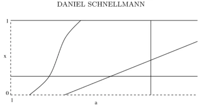
!"# !"## !"$ −%"# −% −!"# ! !"# % %"# !"## !"#$ !"#& !"#' −!"%# −!"% −!"!# ! !"!# !"% !"%#
Figure 1.1: Sample of 200 randomly chosen curves λ !→ Y
λ, λ ∈
[2
−1,
2
−2/3], and a zoom on it.
Peres and Solomyak claimed that their simplified proof in [PS]
would be better suited to analyze more general random power series.
In Paper C we have shown that, indeed, the approach of Peres and
Solomyak does apply to certain variants of the original problem —
namely, when the λ
nare replaced by λ
ϕ(n)for certain well-behaved
functions ϕ : N → R. In the light of the tremendous amount of
atten-tion the
!
±λ
nproblems have received and continuous to receive, it
is very natural to explore variants such as the ones proposed by Paper
C.
To conclude this section, we would like to mention a recent result
by Tsujii [Ts] already referred to in Section 1.1. In [Ts], Tsujii applies
in an ingenious way the idea in Peres and Solomyak’s paper, that a
geometric transversality condition implies absolute continuity, to
par-tially hyperbolic surface endomorphisms F : M → M, where M is, say,
the two-dimensional torus T
2= R
2/Z
2. We call µ a physical measure
for F if the set of points x ∈ M such that
1
n
n−1!
i=0δ
Fi(x) weak-∗−→
µ,
as n → ∞,
has positive Lebesgue measure. (In the terms of Paper D, one could say
that µ is a physical measure if the set of points x ∈ M which are typical
for µ has positive Lebesgue measure.) In [Ts] it is shown that,
gener-ically, such a partially hyperbolic surface endomorphism has a finite
number of ergodic physical measures, whose basins cover Lebesgue a.e.
point of M. Furthermore — here appears essentially the idea in [PS]
— these physical measures are absolutely continuous w.r.t. Lebesgue
measure on M if the sum of their Lyapunov exponents is positive. This
is a true novelty since, usually, absolute continuity is a result of
expan-sion in all directions. To obtain absolute continuity in the case when
the central Lyapunov exponent is zero or even negative, Tsujii makes
use of a similar geometric transversality property as in [PS], which is
generically satisfied in the space of surface endomorphisms. More
pre-cisely, the intuitive picture is the following. Let F : M → M be a
partially hyperbolic surface endomorphism and ν an ergodic physical
measure with central Lyapunov exponent equal to zero or sufficiently
close to zero (it might be negative). It is shown, that, due to the
dominating expansion in the unstable directions E
u, ν is attained as a
weak-∗ limit point of the sequence
1
n
n−1!
i=0ν
γ◦
F
−i,
as n → ∞,
where ν
γis a smooth measure on a curve segment γ of an unstable
manifold. Zooming in on a small neighborhood of a point in the support
of ν, the image F
n(γ) should roughly be comparable to the right figure
in Figure 1.1. The curves in this neighborhood would not concentrate
in the central direction strongly, as the central Lyapunov exponent is
nearly neutral (almost everywhere w.r.t. ν). By a certain control of
the angles between intersecting curves in F
n(γ) — this is generically
provided by the transversality property — Tsujii deduces that in fact
the measure ν is absolutely continuous.
Heuristically, regarding the Bernoulli convolutions considered in
[PS], the numbers log 2
−1and log λ
−1correspond to the Lyapunov
ex-ponents in [Ts], where log 2
−1corresponds to the central Lyapunov
exponent (the 2 comes from the distribution of µ). Their sum is
pos-itive for λ > 2
−1, in which case one has indeed almost sure absolute
continuity. On the other hand, for λ < 2
−1, ν
λis singular as it is
mentioned in Paper C.
1.3
Absolutely continuous limit
distributions of sums of point
measures
The results in Papers D and E are essentially inspired by the last
chapter, Chapter III, of Benedicks and Carleson’s paper [BC1] on the
quadratic map f
a(x) = 1 − ax
2, x ∈ (−1, 1), where they prove that
for Lebesgue almost every parameter value a in a positive Lebesgue
measure set ∆
∞⊂
(1, 2), constructed in the previous two chapters in
[BC1], the map f
aadmits an a.c.i.p. µ
a. More precisely, in Chapters I
and II in [BC1] they construct in an inductive way a positive Lebesgue
measure Cantor set ∆
∞of a-values such that the associated maps f
ahave certain expansion properties along the forward orbit of the critical
point 0. An important ingredient of this construction is the fact that,
for j ≥ 1, the a-derivative ∂
af
aj(1) and the x-derivative ∂
xf
aj(1) are
comparable if a ∈ ∆
∞. In Chapter III these expansion properties in
the a-direction are then used to show that for Lebesgue a.e. parameters
a ∈
∆
∞a limit distribution µ
aof the forward orbit of the critical point
exists and is absolutely continuous w.r.t. Lebesgue measure. Even if
the techniques in Chapter III of [BC1] turn out to be very powerful,
they have, to the best of the authors knowledge, not been used in other
contexts than the quadratic maps. Papers D and E provide us with
several non-trivial, elementary, and important examples where these
techniques can be applied.
In the remaining part of this section we will present the main
tech-nical ingredient of the result in Chapter III in [BC1] — and as well
of the results in Papers D and E — by showing for the doubling map
T
(x) = 2x mod 1, x ∈ [0, 1], the well-known fact that for Lebesgue a.e.
point x ∈ [0, 1] the weak-∗ limit of the sequence
1
n
n!
j=1δ
Tj(x)(1.6)
exists and coincides with the Lebesgue measure m on [0, 1]. This
exam-ple provided by the doubling map can serve as a toy model for Paper D
as well as for Paper E (cf. summaries of Papers D and E below). The
Lebesgue measure m is the unique (and hence ergodic) a.c.i.p. for the
map T . Thus, the fact we are going to show with the techniques used
in [BC1] follows also straightforward from Birkhoff’s ergodic theorem.
Now, let
B :=
"(x − r, x + r) ∩ [0, 1] ; x ∈ Q, r ∈ Q
+# ,
and for each B ∈ B consider the function
F
n(x) =
1
n
n!
j=1χ
B(T
j(x)),
n ≥
1,
x ∈
[0, 1],
which counts the average number of visits to the interval B during
the first n iterations of x. The main observation is summarized in
the following lemma. Its proof is elementary (see, e.g., Lemma A.1 in
Paper E).
Lemma 1.3.1.
Let B ∈
B and assume that there are positive constants
K and C such that for all h ≥
1 there is an integer n
h,Bsuch that
$
[0,1]
whenever n ≥ n
h,B. If the sequence n
h,Bcan be chosen to grow at most
exponentially in h, then it follows that
lim
n→∞
F
n(x) ≤ C|B|,
(1.8)
for Lebesgue a.e. x ∈ [0, 1].
If (1.8) holds for all B ∈ B, then it follows, by standard measure
theory, that for a.e. x ∈ [0, 1] every measure µ
xobtained as a weak-∗
limit point of
1
n
n!
j=1δ
Tj(x)has a density, which is bounded above by C and, in particular, µ
xis
absolutely continuous. Note that, by construction, µ
xis an invariant
probability measure for T . Since the Lebesgue measure m is the unique
a.c.i.p. for T , it follows that µ
xin fact coincides with m and that the
weak-∗ limit of (1.6) exists. Thus, we only have to show that for each
B ∈ B inequality (1.7) is satisfied where the sequence n
h,Bgrows at
most exponentially in h. We write
"
[0,1]F
n(x)
hdx
=
!
1≤j1,...,jh≤n1
n
h"
[0,1]χ
B(T
j1(x)) · · · χ
B(T
jh(x))dx. (1.9)
Assume that we have proven the following proposition.
Proposition 1.3.2.
For all B ∈ B and h ≥ 1 there is an integer
n
h,B, growing for fixed B at most exponentially in h, such that, for all
n ≥ n
h,Band for all integer h-tuples
(j
1, ..., j
h) with 1 ≤ j
1< j
2< ... <
j
h≤ n and j
l− j
l−1≥
√
n, l
= 2, ..., h, we have
"
[0,1]
χ
B(T
j1(x)) · · · χ
B(T
jh(x))dx ≤ (2|B|)
h.
(1.10)
Remark
1.3.3. As we are going to see in the proof of this proposition, we
could state it in a stronger version. More precisely, we could drop the
dependence of n
h,Bon h and, hence, it would be enough to require that
only dependent on B. This is due to the very special properties of
the doubling map. However, we are not able to prove such a stronger
version in the cases considered in Papers D and E. Since we want to
refer to such a toy model as provided by this example with the doubling
map, we stated Proposition 1.3.2 in this weaker form.
From a probabilistic point of view, Proposition 1.3.2 says that if
the distances between the j
l’s are sufficiently large, then the functions
χ
B(T
Bjl(x))’s can be seen as independent random variables. In fact,
since the doubling map with the invariant measure m is exact and,
hence, mixing of all degrees, the integral in (1.10) converges to |B|
has
n tends to infinity (instead of 2 in the right hand side of (1.10), we could
take any real number strictly greater than 1). Note that, for h
≥ 2, the
number of h-tuples (j
1, ..., j
h) in (1.9) for which min
k!=l|j
k− j
l| <
√
n
is bounded by 2h
2n
h−1/2. Hence, by Proposition 1.3.2, we obtain, for
h
≥ 1,
!
[0,1]F
n(x)
hdx
≤ (2|B|)
h+
2h
2√
n
≤ 2(2|B|)
h,
if
n
≥ max
"
n
h,B,
#
2h
2(2|B|)
h$
2%
.
Since both terms in this lower bound for n grow at most exponentially
in h, this concludes the proof of (1.7).
To conclude this section we prove Proposition 1.3.2.
Proof.
Set τ
B= log(2/|B|)/ log 2, and let n
h,B(= n
B) be an integer
such that √n
h,B≥ τ
B. By P
j, j
≥ 1, we denote the open intervals of
monotonicity for T
j: [0, 1]
→ [0, 1], i.e. P
j
= {(k/2
j, (k + 1)/2
j) ; 0
≤
k < 2
j}. We set P
0
= (0, 1) and if Ω is a subset of monotonicity
intervals in P
j, j
≥ 0, then we write P
j+l|Ω, l
≥ 0, for the intervals in
P
j+l, which are also contained in an interval of Ω. Set Ω
0= (0, 1) and,
for 1
≤ l ≤ h, we define
Ω
l= {ω
∈ P
jl+τB|Ω
l−1; T
jl
(ω)
∩ B (= ∅}.
Observe that the set we are interested in, i.e. the set
{x
∈ [0, 1] ; T
jl(x)
is contained in Ω
h(disregarding a finite number of points). If n ≥ n
h,B,
then we have j
l−j
l−1≥ τ
B, 2 ≤ l ≤ h, and we obtain, by the definitions
of τ
Band Ω
l, 1 ≤ l ≤ h,
Ω
l⊂
{x ∈ Ω
l−1; T
jl(x) ∈ 2B},
where 2B denotes the interval twice as long as B and having the same
midpoint as B. Thus, by the piecewise linearity of T
jl−jl−1, 1 ≤ l ≤ h
(where we set j
0= 0), we get
|Ω
l| ≤ 2|B||Ω
l−1|,
(1.11)
which implies
|Ω
h| ≤ (2|B|)
h|Ω
0| = (2|B|)
h.
Chapter 2
Summary
2.1
Overview of Paper A –
Non-continuous weakly expanding
skew-products of quadratic maps
with two positive Lyapunov
exponents
We will use the notions from Section 1.1 above. Regarding (1.1), we
let F be the Viana map with base dynamics g(θ) = dθ mod 1 and
coupling function s(θ) = sin(2πθ). In Paper A, instead of integer d’s,
we allow d to be any real number provided that the expansion in the
base dynamics g dominates the vertical expansion. We show that, as in
the cases considered in [Vi] and [BST], we still have positive Lyapunov
exponents.
Theorem 2.1.1.
There exists R
0= R
0(a
0) < 2 such that for any real
number d > R
0, for every sufficiently small α >
0, F has a positive
vertical Lyapunov exponent at Lebesgue almost every point in !
J .
Furthermore, for a full Lebesgue measure set of d’s considered in
Theorem 2.1.1, the existence of an a.c.i.p. is shown.
Theorem 2.1.2.
For Lebesgue a.e. d > R
0, for every sufficiently
small α >
0, F admits a unique a.c.i.p. µ, where the basin of µ has
full Lebesgue measure in !
J.
The main technical novelty in Paper A is the introduction of the
concept of remainder intervals. Let g : [0, 1) → [0, 1) be the map in
the base dynamics as defined above, i.e. g(θ) = dθ mod 1, and denote
by P
nthe monotonicity intervals of g
n
: [0, 1) → [0, 1). A remainder
interval in P
nis a monotonicity interval of g
n
having not full length, i.e.
its size is smaller than d
−n. The first observation, stated in Lemma 3.2
in Paper A, is that the number of remainder intervals in P
ncan grow
in n at most proportionally to the number of entire intervals in P
n,
which are monotonicity intervals of g
nof full length, i.e. their size is
equal to d
−n. This implies then that there is a constant C ≥ 1 such
that, for all d > R
0,
#{monotonicity intervals in P
n} ≤ Cd
n,
(2.1)
for all n ≥ 1. Furthermore, this fact persists when one zooms in on a
subinterval I of [0, 1], i.e.
#{monotonicity intervals ω ∈ P
n; ω ∩ I &= ∅} ≤ C
′d
n|I|,
(2.2)
for some constant C
′≥ 1 and provided that n is sufficiently large (see
Lemma 3.3 in Paper A). The facts (2.1) and (2.2) suggest that we can,
virtually, assume that the monotonicity intervals of g
nhave full length,
and, thus, we are in a very similar situation as in the case when d is
an integer.
Remark
2.1.3. The property that one can neglect too short intervals is
also used in Paper D. It is reflected in condition (III) stated in Paper D,
which the one-parameter families therein have to fulfill.
Theorem 2.1.2 follows from a result due to Alves [Al]. In [Al] it is
shown that maps contained in a certain family of piecewise expanding
maps φ : !
J
→ !
J
, which have not a finite but a countable number of
pieces of continuity, admit an a.c.i.p. An essential property of maps φ
contained in this family is that the image by φ of a domain of continuity
for φ should be large. Regarding the Viana map F , in [Al] a piecewise
expanding map φ is constructed in a way such that its continuity
do-mains R are of the form R = ω × I, ω ∈ P
nand I an interval, and
such that φ restricted to R is identical to the n-th iteration of F , i.e.
φ|
R≡
F
n
. Furthermore, the construction is made such that the
ver-tical length of φ(R) is sufficiently large. Now, the additional difficulty
for non-integer d’s is that the horizontal length of φ(R) = F
n(ω × I)
is small whenever |ω| ≪ d
−n. To avoid that elements ω associated
to the continuity domains of φ are too small one has to prevent that
points θ ∈ [0, 1] are too often contained in a too short monotonicity
interval of g
nwhen n increases. For this purpose it turns out that it is
enough to have a good control of the forward orbit by g of the point 1
(see Lemma 8.3 in Paper A and its proof). Due to a result of
Schmel-ing [Sch], the distribution of the forward orbit of 1 coincides with the
a.c.i.p. of g for Lebesgue a.e. d > 1, which provides us then with a
sufficiently good information of the forward orbit of 1 — at least for
Lebesgue a.e. d > 1.
Remark
2.1.4. The key lemma in proving Theorem 2.1.2 is Lemma 8.3
in Paper A. A similar lemma could be proved for the C
2-versions of
the β-transformation considered in Section 5 of Paper D. To do so, one
has to replace Lemma 8.4 in Paper A by condition (IIa) in Paper D
and Lemma 8.5 in Paper A, which is the above mentioned result due
to Schmeling [Sch], by Corollary 5.4 in Paper D, where the map X
in this corollary is taken as in its following Remark 5.5. Thus, if we
took, instead of the base dynamics g, a one-parameter family T
aas
de-scribed in Section 5 of Paper D, one could expect to get a result analog
to Theorem 2.1.2, provided of course that a corresponding version of
Theorem 2.1.1 holds. One obstacle of proving Theorem 2.1.1 in this
new setting is that one has to consider high derivatives of the
admissi-ble curves if the expansion of T
ais too weak. However, assuming that
the family T
ais strongly expanding (as it is done in [Vi]) and taking as
the coupling function the linear map θ %→ 2θ − 1, instead of sin(2πθ),
it would be sufficient, in the proof of an analog of Theorem 2.1.1, to
look only at the first derivative of an admissible curve. Combined with
standard distortion estimates for piecewise expanding interval maps,
one should be able to derive a positive vertical Lyapunov exponent
also in the case when one has a C
2-version of the β-transformation in
the base dynamics.
2.2
Overview of Paper B – Positive
Lyapunov exponents for quadratic
skew-products over a
Misiurewicz-Thurston map
We will use the same notations as in Section 1.1 above. Let 1 <
a
1≤
2 be a parameter such that the quadratic map f
a1(x) = a
1−
x
2
is Thurston. Regarding (1.1), we take the
Misiurewicz-Thurston map f
a1as the base dynamics. But in order to have a strong
enough horizontal expansion, we choose instead of f
a1a sufficiently
high iteration of f
a1, i.e. we set g(x) = f
k
a1
(x) for some k ≥ 1. Let
p
1be the unique negative fixed point for f
a1. In Paper B we consider
skew-products
F
: [p
1, −p
1] × R → [p
1, −p
1] × R
(θ, x) &→ (f
ak1(θ), f
a0(x) + αs(θ)),
where α > 0 is chosen sufficiently small and the coupling function
s
: [p
1, −p
1] → [−1, 1] is a priori not fixed. Like for the map considered
in Paper A, there is an open interval (−1, 1) ⊂ I ⊂ (−2, 2) such that
F
([p
1, −p
1] × I) ⊂ [p
1, −p
1] × I, provided α is sufficiently small. We
denote this F -invariant region [p
1, −p
1] × I by !
J
. The main result in
Paper B is the following.
Theorem 2.2.1.
There exist a piecewise C
1coupling function s
:
[p
1, −p
1] → [−1, 1] and an integer k
0≥
1 such that, for all sufficiently
small α >
0 and all k ≥ k
0, the map F
: !
J → !
J :
F
(θ, x) = (f
ak1(θ), f
a0(x) + αs(θ))
For a short illustration of the proof of Theorem 2.2.1 we consider
the situation when a
1= 2, in which case p
1= −1 and the map f
a1:
[−1, 1] → [−1, 1] is conjugated by the map ϕ(θ) = 2π
−1arcsin(θ), θ ∈
[−1, 1], to the symmetric tent map with slope 2, i.e. ϕ ◦ f
a1◦
ϕ
−1
(θ) =
1−2|θ|. Set T (θ) = 1−2|θ| and let h : [−1, 1] → [−1, 1] be an arbitrary
C
1map whose first derivative is uniformly bounded away from 0, i.e.
there exists a constant K
1≥
1 such that K
1−1≤
|h
′(θ)| ≤ K
1, θ ∈
[−1, 1]. Now, setting s(θ) = h(ϕ(θ)) and conjugating the associated
function F with the conjugation function Φ(θ, x) = (ϕ(θ), x), we obtain
˜
F
(θ, x) = Φ ◦ F ◦ Φ
−1(θ, x) = (T
k(θ), f
a0(x) + αh(θ)).
Note that if we show two positive Lyapunov exponents for the map
˜
F
, then it immediately follows that F admits two positive Lyapunov
exponents. In contrast to F , the base dynamics of ˜
F
is now a piecewise
linear and uniformly expanding map and the coupling function h for
˜
F
has bounded derivatives. This makes ˜
F
very similar to the systems
studied by Viana and we are able to make use of the methods in [Vi]
to prove positive Lyapunov exponents for ˜
F
. The fact that the
deriva-tive of h is bounded away from 0 makes it sufficient to look at the
first derivative of the admissible curves, provided that T
kis strongly
expanding (which is the case if k is chosen so large that 2k ≥ 5K
1+ 4).
For general Misiurewicz-Thurston parameters a
1we can apply a
similar conjugation for f
a1as above to obtain in the base dynamics an
expanding map, which expansion is uniformly bounded away from 1.
The existence of such a conjugation function was firstly noted by Ognev
[Og]. In [Og] it is shown that for each Misiurewicz-Thurston parameter
a
1there exists a piecewise analytic function ϕ : [p
1, −p
1] → [−1, 1] such
that for every D > 1 there is an integer k
0≥
1 such that
|(ϕ ◦ f
k a1◦
ϕ
−1
)
′(θ)| ≥ D,
for all k ≥ 1 and all θ for which the derivative is defined (see
Propo-sition 2.2 in Paper B). By piecewise analytic we mean here that,
dis-regarding a finite number of points, the interval [p
1, −p
1] can be
par-titioned into a finite number of open intervals on each of which the
function ϕ is analytic. If a
1<
2 then the conjugated function T (θ) =
ϕ ◦
f
ka1
◦
ϕ
−1is not any longer piecewise linear. Further, in contrast to
the case when a
1= 2, there are more than two points in [p
1, −p
1] such
that |ϕ
′(θ)| tends to ∞ when approaching them (at least from one side).
This causes then that the derivative of T is not any longer bounded
and, thus, we have to establish appropriate distortion estimates for the
map T . Misiurewicz-Thurston or more generally Misiurewicz maps are
well-studied, going back to a fundamental paper by Misiurewicz [Mi].
In this paper we made use of some distortion estimates for Misiurewicz
maps due to van Strien [Str] (see Lemma 3.1 in Paper B).
2.3
Overview of Paper C – Almost sure
absolute continuity of Bernoulli
convolutions
This is joint work with M. Björklund. For a fixed α > 0 consider the
random series
Y
λ=
!
n≥1
±λ
nα,
0 < λ < 1,
where the signs are chosen independently with probability 1/2. In
Paper C we are interested in the distribution ν
λof Y
λ. For the case
when 0 < α < 1/2, Wintner [Wi] considered the Fourier transform
of the measure ν
λ, which can be represented as a convergent infinite
product: ˆ
ν
λ(t) =
"
∞ n=1cos(λ
nαt). Since cos(λ
nαt) ≤ 2/3, if 1 ≤ λ
nαt ≤
2, it follows that
|ˆ
ν
λ(t)| ≤ (2/3)
K(t),
where K(t) = #{n ; 1 ≤ λ
nαt ≤ 2}. A minor calculation yields that,
for 0 < α < 1/2, the term (2/3)
K(t)decreases faster than polynomially
in t and thus, for each 0 < λ < 1 the distribution of ν
λis absolutely
continuous and the density is smooth. This method seems to break
down at α = 1/2. Other easy cases are when α > 1 and λ ∈ (0, 1) or
when α = 1 and λ ∈ (0, 1/2). In these cases, the measure ν
λis singular
(see [KW], criteria (10)). In contrast, the situation when α = 1 and
λ ∈
(1/2, 1) turns out to be much harder. It took over half a century
until Solomyak [So] finally settled (with Fourier transform methods) a
conjecture by Erdös which claimed that in this case ν
λis absolutely
continuous for Lebesgue a.e. λ ∈ (1/2, 1) (in [So] it is also shown that
the density of ν
λis in L
2). Shortly after, Peres and Solomyak [PS] gave
a simpler proof of this result. The techniques of this simpler proof
are presented in Section 1.2 above. In Paper C we make use of these
methods, developed by Peres and Solomyak, and we are able to extend
their result to more general Bernoulli convolutions Y
λ. For instance,
we cover the intermediate case when 1/2 ≤ α < 1, in which case we
show that ν
λis absolutely continuous and has a density in L
2, for a.e.
λ ∈
(0, 1). More generally, instead of the sequence n
αin the power of
λ, we consider sequences ϕ(n) of real numbers and prove the following.
Theorem 2.3.1.
Let ν
λbe the distribution of the random series
Y
λ=
!
n≥1
±λ
ϕ(n),
where the signs are chosen independently with probability 1/2. If
lim
n→∞
ϕ(n + 1) − ϕ(n) = 0,
(2.3)
then ν
λis absolutely continuous and has an L
2density, for a.e. λ ∈
(0, 1).
If there exists a constant 0 < β < ∞ such that
lim
n→∞
ϕ(n)
n
= β,
and if the sequence ϕ(n) − βn satisfies (2.3) then there exists a
(non-empty) interval I ⊂ (0, 1) such that ν
λis absolutely continuous and has
an L
2density, for a.e. λ ∈ I.
2.4
Overview of Paper D – Typical
points for one-parameter families of
piecewise expanding maps of the
interval
Let I ⊂ R be an interval and T
a: [0, 1] → [0, 1], a ∈ I, a one-parameter
family of maps of the unit interval, which are uniformly expanding and
piecewise C
2or piecewise C
1with a Lipschitz derivative. We assume
that the dependence of the family T
aon the parameter a is ’nice’. For
example, for each x ∈ [0, 1] the map a $→ T
a(x) is piecewise C
1on
the interval I. Furthermore, we assume that for each parameter a ∈ I
the map T
ahas a unique absolutely continuous invariant probability
measure µ
a. By Birkhoff’s ergodic theorem, the distribution of the
forward orbit of µ
a-almost every x ∈ [0, 1] is described by the measure
µ
a, i.e.
1
n
n−1!
i=0δ
Ti a(x) weak-∗−→
µ
a,
as n → ∞.
(2.4)
If (2.4) holds for a point x ∈ [0, 1], then we say that x is typical for
the measure µ
a. In Paper D we address the question whether a similar
fact, as this one derived from Birkhoff’s ergodic theorem, holds when
we fix a point x ∈ [0, 1] and vary the parameter a, i.e. whether a given
point x ∈ [0, 1] is typical for µ
afor Lebesgue a.e. parameter values
a ∈ I. Or more generally, if X : I → [0, 1] is a C
1map, what kind of
conditions are sufficient to put on X and T
asuch that we are able to
deduce that X(a) is typical for µ
a, for Lebesgue a.e. a ∈ I?
We will consider some examples. Given a map X : I → [0, 1] we
denote by x
j: I → [0, 1], j ≥ 0, the map x
j(a) = T
aj(X(a)). The most
simple example is the case when the family T
ais constant. Regarding
the example of the doubling map treated in Section 1.3 above, we set
for instance T
a(x) = 2x mod 1, where a is contained in some interval
I
. The a.c.i.p. µ
ais in this case the Lebesgue measure m on the unit
interval. If x ∈ [0, 1] is a point which is not typical for m and if we
choose X(a) ≡ x, then X(a) is not typical for m for any parameter
a ∈ I. Note that for this choice of X(a) the derivative of x
jis zero
on I for all j ≥ 0. Let now X : I → [0, 1] be a map whose derivative
does not vanish on I. On the one hand, it follows directly from the
fact that a.e. x ∈ [0, 1] are typical for m that also X(a) is typical
for m for a.e. parameter a ∈ I. On the other hand, considering x
jinstead of T
jin Section 1.3, it is possible to show that X(a) is typical
for m for a.e. parameter a ∈ I by almost the very same proof as it
is given in Section 1.3 (one only has to replace T
j: [0, 1] → [0, 1] by
x
j: I → [0, 1] and adjust slightly the proof of Proposition 1.3.2). The
reason for this is that the map x
j: I → [0, 1] inherits the properties
of T
ja
: [0, 1] → [0, 1], by which we mean, in particular, the expanding
and the mixing properties. More precisely, one can show that if the
derivative of X is uniformly bounded away from 0 then, for j sufficiently
large, for any interval ω in I, which is mapped one-to-one onto [0, 1]
by x
j, the map x
j+1◦
x
j|
−1ω: [0, 1] → [0, 1] is almost the doubling map
T
aitself. To make a similar kind of comparison of x
jand T
ajalso work
for other families, it is sufficient to require that the a-derivative and
the x-derivative of T
ja
![Figure 1.1: Sample of 200 randomly chosen curves λ !→ Y λ , λ ∈ [2 − 1 , 2 − 2/3 ], and a zoom on it.](https://thumb-eu.123doks.com/thumbv2/123doknet/14538302.724373/21.892.248.652.347.641/figure-sample-randomly-chosen-curves-λ-y-zoom.webp)
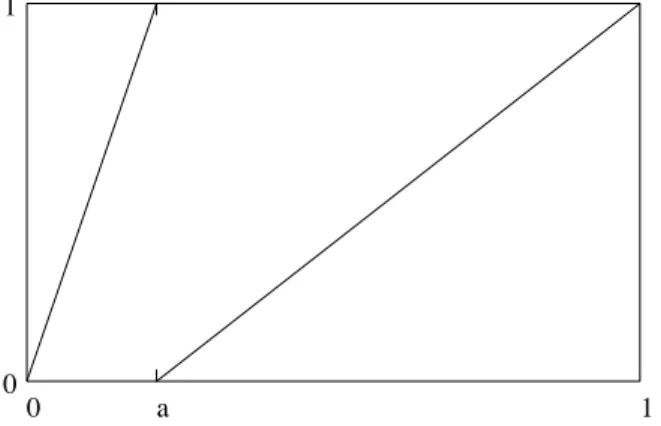
![Figure 1. A possible beginning of a graph for T : [0, ∞ ) → [0, 1].](https://thumb-eu.123doks.com/thumbv2/123doknet/14538302.724373/104.892.156.623.423.702/figure-possible-beginning-graph-t.webp)