RESEARCH OUTPUTS / RÉSULTATS DE RECHERCHE
Author(s) - Auteur(s) :
Publication date - Date de publication :
Permanent link - Permalien :
Rights / License - Licence de droit d’auteur :
Bibliothèque Universitaire Moretus Plantin
Institutional Repository - Research Portal
Dépôt Institutionnel - Portail de la Recherche
researchportal.unamur.be
University of Namur
Habitability of planets on eccentric orbits
Bolmont, Emeline; Libert, Anne Sophie; Leconte, Jeremy; Selsis, Franck
Published in:
Astronomy and Astrophysics DOI:
10.1051/0004-6361/201628073
Publication date: 2016
Document Version
Publisher's PDF, also known as Version of record
Link to publication
Citation for pulished version (HARVARD):
Bolmont, E, Libert, AS, Leconte, J & Selsis, F 2016, 'Habitability of planets on eccentric orbits: Limits of the mean flux approximation', Astronomy and Astrophysics, vol. 591, A106. https://doi.org/10.1051/0004-6361/201628073
General rights
Copyright and moral rights for the publications made accessible in the public portal are retained by the authors and/or other copyright owners and it is a condition of accessing publications that users recognise and abide by the legal requirements associated with these rights. • Users may download and print one copy of any publication from the public portal for the purpose of private study or research. • You may not further distribute the material or use it for any profit-making activity or commercial gain
• You may freely distribute the URL identifying the publication in the public portal ?
Take down policy
If you believe that this document breaches copyright please contact us providing details, and we will remove access to the work immediately and investigate your claim.
A&A 591, A106 (2016) DOI:10.1051/0004-6361/201628073 c ESO 2016
Astronomy
&
Astrophysics
Habitability of planets on eccentric orbits: Limits of the mean flux
approximation
Emeline Bolmont
1, Anne-Sophie Libert
1, Jeremy Leconte
2, 3, 4, and Franck Selsis
5, 61 NaXys, Department of Mathematics, University of Namur, 8 Rempart de la Vierge, 5000 Namur, Belgium
e-mail: [email protected]
2 Canadian Institute for Theoretical Astrophysics, 60st St George Street, University of Toronto, Toronto, ON, M5S3H8, Canada 3 Banting Fellow
4 Center for Planetary Sciences, Department of Physical & Environmental Sciences, University of Toronto Scarborough, Toronto,
ON, M1C 1A4, Canada
5 Univ. Bordeaux, LAB, UMR 5804, 33270 Floirac, France 6 CNRS, LAB, UMR 5804, 33270 Floirac, France
Received 4 January 2016/ Accepted 28 April 2016
ABSTRACT
Unlike the Earth, which has a small orbital eccentricity, some exoplanets discovered in the insolation habitable zone (HZ) have high orbital eccentricities (e.g., up to an eccentricity of ∼0.97 for HD 20782 b). This raises the question of whether these planets have surface conditions favorable to liquid water. In order to assess the habitability of an eccentric planet, the mean flux approximation is often used. It states that a planet on an eccentric orbit is called habitable if it receives on average a flux compatible with the presence of surface liquid water. However, because the planets experience important insolation variations over one orbit and even spend some time outside the HZ for high eccentricities, the question of their habitability might not be as straightforward. We performed a set of simulations using the global climate model LMDZ to explore the limits of the mean flux approximation when varying the luminosity of the host star and the eccentricity of the planet. We computed the climate of tidally locked ocean covered planets with orbital eccentricity from 0 to 0.9 receiving a mean flux equal to Earth’s. These planets are found around stars of luminosity ranging from 1 L to 10−4 L . We use a definition of habitability based on the presence of surface liquid water, and find that most of the planets
considered can sustain surface liquid water on the dayside with an ice cap on the nightside. However, for high eccentricity and high luminosity, planets cannot sustain surface liquid water during the whole orbital period. They completely freeze at apoastron and when approaching periastron an ocean appears around the substellar point. We conclude that the higher the eccentricity and the higher the luminosity of the star, the less reliable the mean flux approximation.
Key words. planets and satellites: atmospheres – planets and satellites: terrestrial planets – methods: numerical
1. Introduction
The majority of the planets found in the insolation habitable zone (HZ, the zone in which a planet could sustain surface liquid wa-ter, as defined byKasting et al. 1993) are on eccentric orbits. The actual percentage depends on the definition of the inner and outer edges considered for the HZ. For instance, about 80% of the planets spending some time in the conservative HZ, whose the inner edge corresponds to the “runaway greenhouse” criterium and the outer edge to the “maximum greenhouse” criterium (e.g.,
Kopparapu 2013;Kopparapu et al. 2014) have an eccentricity of
more than 0.11.
While most of the planets detected in the HZ are very massive planets and are probably gaseous, five of them have masses below 10 M⊕ and eleven of them have radii smaller than 2 R⊕ (such as Kepler-186f with an estimated eccentric-ity of ∼0.01;Quintana et al. 2014). Among these sixteen possi-bly rocky planets, four of them have eccentricities higher than 0.1: GJ 832 c (Bailey et al. 2009), Kepler-62 e, Kepler-69 c
(Borucki et al. 2011), and GJ 667 Cc (Anglada-Escudé et al.
2012; Robertson & Mahadevan 2014). Table 1 shows the
1 http://physics.sfsu.edu/~skane/hzgallery/index.html
characteristics of these four planets and the percentage of the orbital phase spent within the HZ for two different definitions of the inner and outer edges.
We expect more small planets to be discovered in the HZ with the future missions to increase statistics (e.g., NGTS, TESS) and also better constrain eccentricity (e.g., PLATO). In any case, the discovery of the 4 planets mentioned above raise the question of the potential habitability of planets, like GJ 832 c and GJ 667 Cc, that only spend a fraction of their orbit in the HZ.
The influence of the orbital eccentricity of a planet on its climate has already been studied using various methods: energy-balanced models (EBMs) and global climate models (GCMs). EBMs assume that the planet is in thermal equilibrium: on av-erage, the planet must radiate the same amount of long-wave radiation to space as the short-wave radiation it receives from the host star (Williams & Kasting 1997). In EBM models, the radiative energy fluxes entering or leaving a cell are balanced by the dynamic fluxes of heat transported by winds into or away from the cell. On the contrary, GCMs consistently compute on a three-dimensional grid the circulation of the atmosphere using forms of the Navier-Stokes equations. GCMs are therefore more
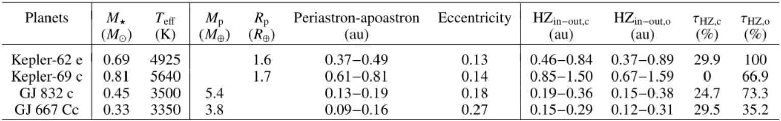
Table 1. Possibly rocky observed exoplanets with an eccentricity higher than 0.1 (from the Habitable Zone Gallery,Kane & Gelino 2012).
Planets M? Teff Mp Rp Periastron-apoastron Eccentricity HZin−out,c HZin−out,o τHZ,c τHZ,o
(M ) (K) (M⊕) (R⊕) (au) (au) (au) (%) (%)
Kepler-62 e 0.69 4925 1.6 0.37−0.49 0.13 0.46−0.84 0.37−0.89 29.9 100 Kepler-69 c 0.81 5640 1.7 0.61−0.81 0.14 0.85−1.50 0.67−1.59 0 66.9 GJ 832 c 0.45 3500 5.4 0.13−0.19 0.18 0.19−0.36 0.15−0.38 24.7 73.3 GJ 667 Cc 0.33 3350 3.8 0.09−0.16 0.27 0.15−0.29 0.12−0.31 29.5 35.2
Notes. HZin−out,ccorresponds to the inner and outer edge of the conservative HZ and HZin−out,ocorresponds to the inner and outer edge of the
optimistic HZ (the inner edge corresponds to the “recent Venus” criterium and the outer edge to the “early Mars” criterium; e.g.,Kopparapu 2013;
Kopparapu et al. 2014). τHZ,cis the percentage of the orbital phase spent within the conservative HZ and τHZ,ois the percentage of the orbital phase
spent within the optimistic HZ.
computationally demanding, but they are more accurate when simulating a climate.
Using a GCM, Williams & Pollard (2002) studied the in-fluence of the eccentricity on the climate of Earth-like planets around a Sun-like star (with the correct distribution of continents and oceans, a 365 day orbit, a 24 h day, and a 23◦obliquity) and found that surface liquid water is possible even on very eccen-tric orbits. Using a GCM,Linsenmeier et al.(2015) studied the influence of both obliquity and eccentricity for ocean covered planets orbiting a Sun-like star on a 365 day orbit and a 24 hour day, like Earth. They found that planets with eccentricities higher than 0.2 can only sustain surface liquid water for a part of the year.
Spiegel et al.(2010) andDressing et al.(2010) used EBMs
to illustrate the effect of the evolution of eccentricity (through pseudo-Milankovitch’s cycles; Milankovitch 1941).
Spiegel et al. (2010) found that the increase of eccentricity
of a planet may allow it to escape a frozen snowball state.
Dressing et al. (2010) found that increasing the eccentricity
widens the parameter space in which the planet can only sustain surface liquid water for part of the year.
A major result ofWilliams & Pollard(2002) was that the ca-pacity of an eccentric planet of semi-major axis a and eccen-tricity e to host surface liquid water depends on the average flux received over one orbit. This average flux corresponds to the flux received by a planet on a circular orbit of radius r= a(1 − e2)1/4. If this orbital distance is within the HZ, then the planet is as-sumed to belong to the HZ (or to the eccentric HZ, as defined by
Barnes et al. 2008). However this study was performed by
simu-lating the climate of an Earth-twin planet. The generalization of this result to the diversity of the planets discovered in the HZ is not straightforward. We expect this mean-flux approximation to be adequate for planets with low eccentricities; however, for high eccentricities the climate could be drastically degraded when the planet is temporarily outside the HZ. This would especially be an issue for planets around hot stars where the HZ is far from the star. The planet could spend a long time outside of the HZ, leading to the freezing of the water reservoir at apoastron and its evaporation at periastron.
The influence of the stellar luminosity/host star type has pre-viously been considered for Earth-like planets on circular orbits (e.g., Shields et al. 2013, 2014) and Wordsworth et al. (2011) have studied the climate of GJ 581d orbiting a red dwarf for two different eccentricities (0 and 0.38), but no work has studied jointly the influence of the planet’s eccentricity and the stellar luminosity.
We therefore aimed to explore here, in a systematic way, the influence of the planet’s eccentricity and the star luminosity
on the climate of ocean covered planets in a 1:1 spin-orbit resonance, that receive on average the same flux as Earth. In order to test the limits of the mean flux approximation, we per-formed three-dimensional GCM simulations for a wide range of configurations: we considered stars of luminosity 1 L , 10−2L and 10−4 L and orbits of eccentricity from 0 to 0.9. We took into account the different luminosities by scaling the orbital pe-riods of the planets. This means that we did not consider here the spectral dependance of the stars. We investigated whether these planets were able to sustain surface liquid water.
In Sect.2we present our definition of habitability in terms of surface liquid water coverage. In Sect.3we explain the set-up of our simulations, and in Sects.4and5we discuss their out-come in terms of liquid water coverage. In Sect.7we discuss the observability of the variability caused by eccentricity. Finally, in Sects.8and9we conclude this study.
2. Liquid water coverage vs. habitability
We do not consider that habitability is equivalent to the re-quirement of having a mean surface temperature higher than the freezing point of water, as do the energy balance models (e.g.,
Williams & Kasting 1996) or the radiative-convective models
(e.g.,Kasting et al. 1993). As inSpiegel et al.(2008), we chose an assessment of the habitability of a planet based on sea ice cover. We focus here only on the presence of surface liquid wa-ter and not on the actual potential of the planets to be appropriate environments for the appearance of life.
The planets considered in this work are water worlds (or aqua worlds), i.e., planets whose whole surface is covered with water (here treated as an infinite water source). Considering water worlds is especially convenient for a first study because it allows us to have a small number of free parameters (no land/ocean distribution, land roughness, etc.). A subset of this population are the ocean planets with a high bulk water frac-tion, which strongly alters their internal structure. Ocean plan-ets were hypothesized in the early 2000s by Kuchner (2003)
andLéger et al.(2004). They are believed to have a mass
rang-ing from 1 M⊕(small rocky planets) to 10 M⊕(mini-Neptunes). Their composition was investigated, and the depth of the ocean of a Earth-mass planet was estimated to a few hundred kilome-ters (Sotin et al. 2007). These planets could be identified pro-viding that we knew the mass and radius with enough preci-sion (Sotin et al. 2007; Selsis et al. 2007). Despite the lack of knowledge of their mass, some observed planets have been pro-posed to be ocean planets, for example Kepler-62e and -62f (Kaltenegger et al. 2013).
3. GCM simulations 3.1. Model parameters
We performed the climate simulations with the LMDZ2generic global climate model (GCM) widely used for the study of ex-trasolar planets (e.g.,Wordsworth et al. 2010,2011;Selsis et al. 2011) and the paleoclimates of Mars (Wordsworth et al. 2013;
Forget et al. 2013). In particular, we used the three-dimensional
dynamical core of the LMDZ 3 GCM (Hourdin et al. 2006), based on a finite-difference formulation of the primitive equa-tions of geophysical fluid dynamics. A spatial resolution of 64 × 48 × 30 in longitude, latitude, and altitude was set for the simulations.
We assumed that the atmosphere is mainly composed of N2, with 376 ppmv3 of CO2, which corresponds to an Earth-like at-mosphere. The water cycle was modeled with a variable amount of water vapor and ice. Ice formation (melting) was assumed to occur when the surface temperature is lower (higher) than 273 K, and temperature changes due to the latent heat of fusion were taken into account.
We used the high-resolution spectra computed by
Leconte et al.(2013) over a range of temperatures and pressures
using the HITRAN 2008 database (Rothman et al. 2009). We adopted the same temperature grids as inLeconte et al.(2013) with values T = {110, 170, ..., 710} K and the same pressure grids with values p = {10−3,10−2,...,105} mbar. The water volume mixing ratio could vary between 10−7 to 1. The H
2O absorption lines were truncated at 25 cm−1, but the water vapor continuum was included using the CKD model (Clough et al. 1989). As in Leconte et al. (2013), the opacity due to N2–N2 collision-induced absorption was also taken into account.
We used the same correlated-k method as in
Wordsworth et al. (2011) and Leconte et al. (2013) to
pro-duce a smaller database of spectral coefficients suitable for fast calculation of the radiative transfer in the GCM. The model used 38 spectral bands for the thermal emission of the planet and 36 for the stellar emission. In our water world model, we did not take into account the oceanic circulation. We chose an albedo of 0.07 for the surface liquid water and an albedo of 0.55 for the ice and snow.
We considered the influence of some parameters on the out-come of our simulations: the thermal inertia Iocof the oceans and the maximum ice thickness hiceallowed in our model. We tested three combinations: hice= 1 m, Ioc= 18 000 J s−1/2m−2K−1, hice= 10 m, Ioc= 18 000 J s−1/2m−2K−1, hice= 1 m, Ioc= 36 000 J s−1/2m−2K−1.
The results given in Sects.4,5were obtained with the first com-bination, while comparisons with the other two sets of values is performed in Sect. 6. Changing thermal inertia is a way to model the ocean mixed layer depth, which responds quickly to the climatic forcing. This mixed layer varies on Earth with lo-cation and time.Selsis et al.(2013) studied the effect of chang-ing the thermal inertia of hot planets without atmospheres. They showed that increasing the thermal inertia of the surface of such a planet damped the amplitude of its temperature response to the eccentricity-driven insolation variations. They also showed that increasing thermal inertia introduced a lag in the response of
2 Model developed at the Laboratoire de Météorologie Dynamique, the
Z of LMDZ standing for Zoom capability.
3 Parts per million by volume.
the planet with respect to the insolation variations. Imposing the maximum ice thickness allowed in the model is a way to mimic oceanic transports that limit the growth of ice layers. It influ-ences the time it takes to reach equilibrium and the eccentricity-driven oscillations (see Sect.6).
3.2. Planets and initial conditions
We computed the climate of water worlds, initially ice-free, and obtained a mean flux equal to Earth’s (1366 W/m2) on orbits of eccentricity from 0 to 0.9 around stars of different luminosities:
– L? = 1 L , corresponding to our Sun with an effective tem-perature of ∼5800 K;
– L?= 10−2L , corresponding to a M-dwarf of 0.25 M with an effective temperature of ∼3300 K;
– L? = 10−4L , corresponding to a 500 Myr brown-dwarf of mass 0.04 M with an effective temperature of ∼2600 K. We note that we did not take into account in this work the spec-tral dependance of the stars. For instance, we did not consider that a 10−4 L star is much redder than a 1 L star. We took into account the different luminosities only by scaling the orbital period of the planets, as explained in the following.
We considered here planets in a 1:1 spin-orbit resonance, re-gardless of their eccentricity. However, a planet orbiting a 1 L star on a circular orbit and receiving a flux of 1366 W/m2 (i.e., at an orbital distance of 1 au) will not reach a synchronous rota-tion state in less than the age of the Universe. Moreover, if the planet is very eccentric, the probability that it is in synchronous rotation is low. The planet will more likely be either in pseudo-synchronization (pseudo-synchronization at periastron;Hut 1981) or in spin-orbit resonance (Makarov & Efroimsky 2013). The aim of our work was to investigate the effect of eccentricity and lumi-nosity, so we only varied here these two parameters and kept all the others equal. Choosing a synchronous rotation allowed us to have, for a given eccentricity, the exact same insolation evolu-tion for planets orbiting a high luminosity star as a low luminos-ity star. The obliquluminos-ity of the planet was assumed to be zero. In all cases, the simulations were run from an initial ice-free state until runaway greenhouse/glaciation occurred or steady states of thermal equilibrium were reached.
For the different eccentricities, we scaled the orbital period of the planet (the duration of the “year”) to insure that the planet re-ceives F⊕= 1366 W/m2on average. A planet of semi-major axis aand eccentricity e receives an averaged flux over one orbit of F= L?
4πa2√1 − e2, (1)
where L?is the luminosity of the star. In our study, we assume that the planet receives on average F⊕,
F= F⊕= L 4πa2
⊕
= 1366 W/m2, (2)
where a⊕ = 1 au. Thus, we can express the semi-major axis of the planet as a function of eccentricity e and stellar luminosity L?: a= a⊕ (1 − e2)1/4 s L? L · (3)
If we increase the eccentricity of the orbit of the planet, its semi-major axis a increases to ensure it receives on average F⊕. For
Table 2. Planets’ orbit characteristics and received flux for L?= L .
L?= L
Ecc a(au) Peri (au) Apo (au) Porb(day) Flux at peri (W/m2) Flux at apo (W/m2)
0 1.000 1.00 1.00 365.5 1366 1366 0.05 1.001 0.95 1.05 365.9 1517 1241 0.1 1.003 0.90 1.10 366.9 1697 1136 0.2 1.011 0.81 1.21 371.2 2128 954 0.4 1.045 0.63 1.46 390.2 3758 700 0.6 1.119 0.45 1.79 432.1 8447 534 0.8 1.292 0.26 2.33 536.2 33 731 420 0.9 1.516 0.15 2.88 681.4 139 530 378
Notes. a is the semi-major axis defined in Eq. (3). Because the planets are in synchronous rotation, the orbital period (Porbcolumns, given in Earth
days= 24 h) and the rotation period of the planets are equal. Peri denotes the periastron distance and apo the apoastron distance.
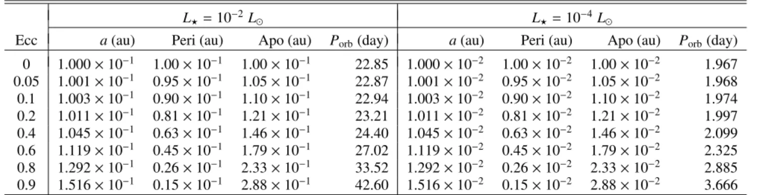
Table 3. Planets’ orbit characteristics for L?= 10−2L and L?= 10−4L .
L?= 10−2L L?= 10−4L
Ecc a(au) Peri (au) Apo (au) Porb(day) a(au) Peri (au) Apo (au) Porb(day) 0 1.000 × 10⁻¹ 1.00 × 10⁻¹ 1.00 × 10⁻¹ 22.85 1.000 × 10⁻² 1.00 × 10⁻² 1.00 × 10⁻² 1.967 0.05 1.001 × 10⁻¹ 0.95 × 10⁻¹ 1.05 × 10⁻¹ 22.87 1.001 × 10⁻² 0.95 × 10⁻² 1.05 × 10⁻² 1.968 0.1 1.003 × 10⁻¹ 0.90 × 10⁻¹ 1.10 × 10⁻¹ 22.94 1.003 × 10⁻² 0.90 × 10⁻² 1.10 × 10⁻² 1.974 0.2 1.011 × 10⁻¹ 0.81 × 10⁻¹ 1.21 × 10⁻¹ 23.21 1.011 × 10⁻² 0.81 × 10⁻² 1.21 × 10⁻² 1.997 0.4 1.045 × 10⁻¹ 0.63 × 10⁻¹ 1.46 × 10⁻¹ 24.40 1.045 × 10⁻² 0.63 × 10⁻² 1.46 × 10⁻² 2.099 0.6 1.119 × 10⁻¹ 0.45 × 10⁻¹ 1.79 × 10⁻¹ 27.02 1.119 × 10⁻² 0.45 × 10⁻² 1.79 × 10⁻² 2.325 0.8 1.292 × 10⁻¹ 0.26 × 10⁻¹ 2.33 × 10⁻¹ 33.52 1.292 × 10⁻² 0.26 × 10⁻² 2.33 × 10⁻² 2.885 0.9 1.516 × 10⁻¹ 0.15 × 10⁻¹ 2.88 × 10⁻¹ 42.60 1.516 × 10⁻² 0.15 × 10⁻² 2.88 × 10⁻² 3.666
Notes. The fluxes at periastron and apoastron are the same as in Table2.
example, a planet around a Sun-like star with an eccentricity of 0.6 and receiving 1366 W/m2 on average has a semi-major axis of 1.119 au.
Table2shows the different values of the semi-major axis of the planets for different eccentricities, as well as the distances of periastron and apoastron, and the fluxes the planet receives at these distances for L? = L . Table3 shows the planets’ orbit characteristics for L? = 10−2L and L? = 10−4 L . Since we consider synchronous planets, we can deduce the rotation period of the planets depending on the eccentricity and the type of the star. For a star of L? = 1 L and a planet on a circular orbit, the year is 365 days long and the planet has a slow rotation. If the planet is on a very eccentric orbit (e = 0.9), then the semi-major axis is 1.516 au, the year is 681 days long, and the planet has an even slower rotation. For a star of L? = 10−4 L and a planet on a circular orbit, the semi-major is 0.01 au, the year is ∼2 days long (∼4 days for e= 0.9), and the planet has a faster rotation.
In addition, as shown inSelsis et al.(2013), because of the optical libration due to the 1:1 spin-orbit resonance, there is no permanent dark area on a planet with an eccentricity higher than 0.72. We define here the dayside as the hemisphere that is il-luminated when the planet has an eccentricity of 0. For this case, the substellar point is at 0◦longitude and 0◦latitude, and the day-side extends to −90◦to 90◦in longitude and −90◦to 90◦in lati-tude. The nightside is the other side of the planet, i.e., from 90◦ to 270◦in longitude and −90◦to 90◦in latitude. We use this geo-graphic definition of the dayside and nightside independently of the eccentricity of the orbit.
We first discuss the effect of varying the star luminosity on the climate of planets on circular orbits (Sect.4), then we extend the discussion to planets on eccentric orbits (Sect.5).
4. Circular orbits
In Sect. 4.1, we first give our results for a star of luminosity L? = 1 L . In Sect.4.2, we compare them with those obtained for a star of luminosity L?= 10−2L and L?= 10−4L .
4.1. L?= 1 L
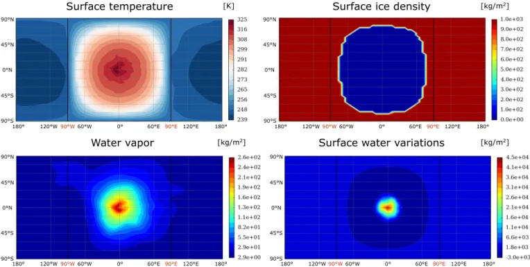
Figure1shows the longitude-latitude maps of surface tempera-ture, ice density, water vapor, and precipitation on a planet or-biting a Sun-like star after 10 000 days. The mean surface tem-perature needs about ∼1500 days to reach its equilibrium, which is about 267 K. As the planet is in synchronous rotation, the dayside is much hotter than the nightside (Fig.1, top left). The temperatures on the dayside reach 320 K at the substellar point, whereas temperatures on the nightside are around 240 K. From an initially free water ocean, an ice cap forms in a few hundred years (Fig. 1, top right). About 62% of the planet is covered with ice and 38% of the ocean remains free of ice around the substellar point. We obtain the same kind of features as an eye-ball planet (like in Pierrehumbert 2011 andWordsworth et al. 2011 for GJ 581d). Evaporation occurs on a ring around the substellar point (Fig.1, bottom right), and there is a lot of pre-cipitation at the substellar point owing to humidity convergence
Surface ice density [kg/m2]
Surface water variations
Water vapor [kg/m2] [kg/m2]
Surface temperature [K]
Fig. 1.Maps of surface temperature, ice density, amount of water vapor integrated on a column, and precipitation for a planet around a 1 L star on
a circular orbit. The terminator (the longitudes of 90◦
W and 90◦
E) is shown in black. For the map showing the surface water variation, a negative value means that liquid water disappears (evaporation or freezing) and a positive value means that liquid water appears (rain or melting). For the map showing the surface ice density, a density of 1000 kg/m2corresponds to a 1000 mm= 1 m thick ice layer.
and condensation of moisture along the ascending branch of an Hadley type cell (Fig.1, bottom left).
The albedo of the planet is about 0.25, which is significantly lower than inYang et al. (2013). This might be due to several differences in our simulations. For example, the albedo depends on the size of the cloud-forming ice grains. The bigger they are, the lower the albedo. In our model, the cloud ice particles have a size that varies depending on the water mixing ratio (see
Leconte et al. 2013for details). InYang et al.(2013) the size is
not indicated, but is said to be the same size as observed on Earth. Furthermore,Yang et al.(2013) pointed out that the albedo of the planet strongly depends on the oceanic transport, which is not in-cluded here. Finally, the biggest difference comes from the moist convection parametrization, which is chosen to be very sim-ple with few free parameters in LMDZ (Manabe & Wetherald 1967). This parametrization leads to a lower cloud cover, and thus a lower albedo.
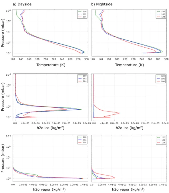
Figure2 shows the dayside and nightside mean profiles of temperature, water ice, and water vapor in the atmosphere. These mean profiles were obtained by performing a time average over one orbital period4. The surface dayside temperatures are higher
than the surface nightside temperatures. Thanks to this lower surface temperature, we can see a temperature inversion on the nightside, which occurs at a pressure level of about 1 bar. On the dayside, water ice clouds are located around an altitude of ∼15 km (∼90 mbar), while on the nightside, there are no water ice clouds in the atmosphere. The concentration of water vapor is much higher on the dayside than on the nightside. For both the dayside and nightside, the water vapor in the atmosphere is
4 54 points per orbit were used for the case 1 L
(Porb = 365.5 day),
122 points for 10−2L
(Porb = 22.85 day), and 98 points for 10−4 L
(Porb = 1.967 day). The number of points depends on the output time
frequency.
essentially found within the first 20 km of the atmosphere (pres-sure >0.1 bar).
On average, the concentration of water vapor in the dayside upper atmosphere (pressure <10 mbar) is about 1 × 10⁻⁹kg/m2, which is about 100 times more than the water vapor concen-tration on Earth at the same altitude (Butcher et al. 1992). It is therefore possible that these planets experience little water escape, as on Earth (Lammer et al. 2003; Kulikov et al. 2007;
Selsis et al. 2007). We note that an extreme case for water escape
has been observed for a hot Neptune (Ehrenreich et al. 2015). However, we expect a much lower escape rate here as the planet is located much farther away. There are ice clouds above the substellar point at an altitude of 15 km; these clouds protect the substellar point.Yang et al.(2013) determined that this mecha-nism allows the inner edge of the insolation HZ for synchronous planets to be closer than for non-synchronous planets.
In conclusion, during its orbit a synchronized planet on a circular orbit around a 1 L star always has a part of its ocean ice-free on the dayside (around the substellar point) and covered by an ice cap on its nightside.
4.2. Decreasing the luminosity
Decreasing the stellar luminosity5changes the global character-istics of the planet’s climate, such as the surface temperature map and the surface ice density. The lower the luminosity the bigger the differences with the previous case.
5 We do not take into account the spectral dependance of a low
lumi-nosity star. Decreasing the lumilumi-nosity is done in our work by decreasing the orbital period of the planet, and thus its rotation period (Tables2
103 102 101 10-1 100 Pr essu re ( m ba r) 120 140 160 180 200 220 240 260 280 300 Temperature (K) 120 140 160 180 200 220 240 260 280 300 Temperature (K)
0.0 2.0e-03 4.0e-03 6.0e-03 8.0e-03 1.0e-02 1.2e-02 1.4e-02
h2o vapor (kg/m2)
0.0 2.0e-03 4.0e-03 6.0e-03 8.0e-03 1.0e-02 1.2e-02 1.4e-02
h2o vapor (kg/m2) a) Dayside b) Nightside 103 102 101 10-1 100 Pr essu re ( m ba r) 103 102 101 10-1 100 Pr essu re ( m ba r)
0.0 4.0e-06 8.0e-06 1.2e-05 1.6e-05 2.0e-05 2.4e-05 2.8e-05
h2o ice (kg/m2)
0.0 4.0e-06 8.0e-06 1.2e-05 1.6e-05 2.0e-05 2.4e-05 2.8e-05
h2o ice (kg/m2)
Fig. 2.a) Dayside and b) nightside mean profiles of temperature (top panels), water ice (middle panels), and water vapor (bottom panels) in the atmosphere of a planet on a circular orbit around a 1 L star (L00, in green), a 10−2L star (L02, in blue), and a 10−4L star (L04, in red).
4.2.1. L?= 10−2L
Figure2 shows that there is little difference between the mean temperature profiles at 1 L and 10−2 L . The temperature at low altitudes (pressure>2 mbar) is slightly lower, but in the up-per atmosphere (pressure <2 mbar) it is higher (the difference reaches 10 to 20 K). The water ice clouds follow the same dis-tribution as for a 1 L star, with a high density at an altitude of ∼15 km (∼90 mbar) on the dayside and very few clouds on the nightside. The water vapor distribution is very similar between the luminosities 1 L and 10−2L and the concentration becomes negligible above an altitude of ∼20 km (pressure <100 mbar).
However, owing to the faster rotation, the temperature dis-tribution is different. This is due to the higher Coriolis force that strengthens the mechanisms responsible for the equato-rial super-rotation. The wave-mean flow interaction identified
by Showman & Polvani (2011) and the three-way force
bal-ance identified by Showman et al. (2013, 2015) both affect the atmospheric circulation (see alsoLeconte et al. 2013, for a
discussion of the transition from stellar-antistellar circulation to super-rotation in the specific context of terrestrial planets). Figure 3 shows maps of the atmospheric temperature (color maps) and the wind pattern (with vectors) at an altitude of 10 km (corresponding to a pressure of 305 mbar for 1 L , 301 mbar for 10−2 L , and 190 mbar for 10−4L ). For 1 L , the wind is weak and isotropically transports heat away from the substellar point (stellar/anti-stellar circulation, as shown in Leconte et al. 2013, for a slowly rotating Gl-581c). However, for 10−2L the wind is stronger, especially the longitudinal component, and re-distributes the heat more efficiently toward the east. Thanks to this stronger wind, there is an asymmetry of the surface tem-perature distribution on the planet, so that the east is hotter than the west and the temperature is more homogeneous along the equator. The planet orbiting a 10−2L star is colder at the poles (surface temperature of ∼235 K) than for 1 L star (surface tem-perature of ∼250 K). The wind pattern here is marked by the presence of a Rossby wave typical of the Rossby wave transi-tion region (as defined inCarone et al. 2015, for tidally locked
Longitude La ti tu de 1 L⊙ 10-2 L⊙ 10-4 L⊙ La ti tu de La ti tu de 90°E 90°W 90°E 90°W 90°E 90°W
Fig. 3. Maps of the atmospheric temperature (color map) and winds (vectors are in units of m/s, legend at the top of the graph) at an altitude of 10 km for a planet on a circular orbit around a 1 L star (top), a
10−2L
star (middle), and a 10−4L star (bottom).
planets). InCarone et al.(2015), the Rossby wave transition re-gion for an Earth-size planet is said to occur for a rotation pe-riod of 25 days, which is approximately the rotation pepe-riod here (22.85 days). In the 1 L case, the rotation period was much longer and no Rossby wave could develop (e.g.,Leconte et al.
2013).
Moreover, for 10−2L , the average ice density is similar to the value of the planet orbiting a 1 L star. However, owing to the asymmetric surface temperature due to the Coriolis force, the shape of the ice-free region is slightly different. Figure4shows the shape of the surface ice density for L?= 10−2L (top panel). Although the percentage of the ice-free region remains the same, the ocean for 10−2L reaches slightly lower latitudes and is more extended longitudinally than for 1 L .
Despite these small changes with respect to the case 1 L , a planet on a circular orbit around a 10−2 L star is therefore equally capable of sustaining surface liquid water.
4.2.2. L?= 10−4L
For an even less luminous host body, the differences that ap-peared for the case L? = 10−2 L are accentuated. The temper-ature maps and surface ice density maps show a more longitu-dinal extension than before. Owing to the even higher rotation rate of the planet (rotation period of 2 days, see Table 3), the winds redistribute heat longitudinally from the substellar point
longitude 10-4 L⊙ la ti tu de la ti tu de 10-2 L⊙ 90°E 90°W 90°E 90°W [kg/m2]
Surface ice density
Fig. 4.Maps of the surface ice density for a planet on a circular or-bit around a 10−2L
star (top) and a 10−4L star (bottom). The map
corresponding to the case L?= 1 L is in Fig.1.
and efficiently heat up the nightside of the planet. Figure3shows that the winds are much stronger for the case 10−4L (∼50 m/s vs. ∼25 m/s for 10−2 L and <10 m/s for 10−4 L ) and redis-tribute the heat very efficiently along the equator. In this case, we note the presence of longitudinal wind jets at latitudes of 45◦S and 45◦N and at a pressure level of ∼30 mbar. The wind velocity in the jets can reach almost 120 km/h. As the rotation period is of ∼2 days, the criteria for the Rossby wave to be triggered is met and super-rotation takes place (Showman & Polvani 2011;
Leconte et al. 2013;Carone et al. 2015). As is true for 10−2L ,
the colder regions are the poles, but the temperature here is even lower (a surface temperature about 20 K lower than for 10−2L ). Figure2shows that this super-rotation also causes a longitu-dinal uniformity of the temperature, water ice clouds and water vapor distribution. Indeed, the nightside temperature of the low-est layer of the atmosphere for 10−4L is not as low as for 1 L and 10−2L , and there are many more ice clouds and water vapor on the nightside for 10−4L than for 1 L
and 10−2L .
We note that the evolution of the surface ice density is not as quick as in the previous two cases where the surface ice den-sity reaches its equilibrium in less than a few decades. Here a few thousands days are needed to reach equilibrium. One of the main differences it implies is an initially lower surface ice den-sity for planets around L? = 10−4 L stars than for more lumi-nous objects. First, the ocean’s region survives and forms a belt around the equator with the belt buckle at the substellar point. As the eastward wind loses heat, the eastern regions are hotter than the western regions. After about 700 days of evolution, the ice forms a bridge at 120◦ west, closing the equatorial ocean. Figure4shows that when equilibrium is reached, the shape of the ocean for L? = 10−4 L is very different from the shapes of the other two luminosities. When equilibrium is reached, we find that this planet has an ice-free ocean of a similar size to the previous cases, i.e., about 40% of the planet is ice-free.
Figure5shows the mean surface evolution and mean ice den-sity evolution for planets around the three different host stars. For the circular orbits, we can see that the mean surface temperature
is higher for L?= 10−4L than for L?= 1 L and L?= 10−2L . This is due to the strong winds in the atmosphere of the planet, which chase the clouds that are forming above the substellar point. Without the cloud protection, the surface temperature in-creases. For a tidally locked planet orbiting very low luminos-ity objects, the longitudinal winds are strong and the stabilizing cloud feedback identified byYang et al.(2013) is less efficient. Therefore, one might expect that the HZ of tidally locked plan-ets around very low luminosity stars is not as extended as in
Yang et al. (2013). However, simulations for higher incoming
flux should be performed to verify this claim, in particular to see how the albedo varies with increasing incoming flux. 5. Eccentric orbits
As described in Sect.3.2, we made sure that all planets receive on average the same flux as Earth. Increasing the eccentricity changes significantly the insolation the planet receives over one orbit and it leads to changes in the general characteristics of the climate. The insolation varies over the orbit and the substellar point moves along the equator as a result of the optical libration. Temperature, atmospheric water ice, atmospheric water vapor, and surface ice are influenced by this forcing, as shown in the following.
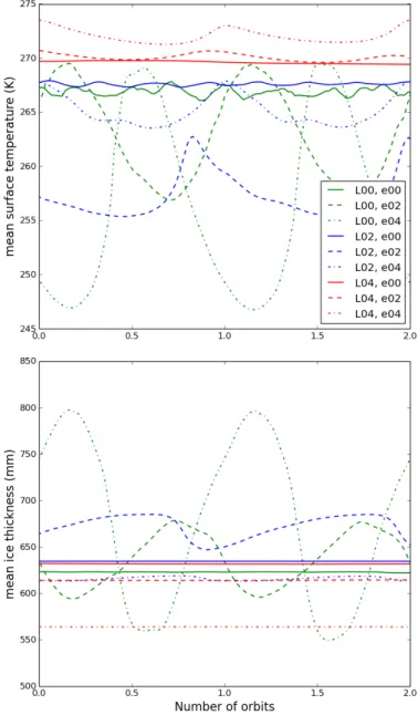
Figure5shows an example of the evolution, during two or-bits, of the mean surface temperature and mean ice thickness for planets on a circular orbit and planets with an eccentricity of 0.2 and 0.4, orbiting the three different object types. The mean sur-face temperature oscillates with the change of insolation over the orbit. As the orbital period changes with the luminosity and eccentricity (see Tables2and3), it oscillates with different fre-quency and amplitude for the different cases. This oscillation of insolation and thus temperature has an effect on the amount of water vapor and surface ice (as seen in Fig.5). We discuss in the following sections the impact on the climate of the planets considered here and the presence of liquid water at their surface. 5.1. Luminosity of L?= 1 L
First, we consider the luminosity of a star similar to the lumi-nosity of the Sun. First, for small eccentricities, our simulations show surface temperature oscillations, ice density, and water vapor oscillations. However, they remain small enough for the planet to keep surface liquid water. For example, a planet on an orbit of eccentricity 0.2 experiences temperature oscillations on the dayside of about 30 K in 371 days, while the mean temper-ature oscillations are of about 12 K (see Fig.5). The surface ice density responds accordingly with the eccentricity-driven sea-sonal melting and freezing. On average, the surface ice density varies between ∼58% after the passage at periastron and ∼66% after the passage at apoastron. The region around the substel-lar point is always ice-free, but the center of the ice-free region shifts on the surface of the planet by about 10◦during the orbit.
Second, when we increase the eccentricity to 0.4, the ampli-tude of the variations is higher. For example, Fig.5shows that the mean temperature variations increase from ∼12 K for an ec-centricity of e = 0.2 to ∼23 K for an eccentricity of e = 0.4. Figure 5 also shows that the amplitude of the mean ice den-sity variations of the planet also increases with the eccentricity. The planet’s surface ice density after periastron is lower than for an eccentricity of 0.2 (∼55% vs. ∼58%), but is much higher af-ter apoastron (∼80% vs. ∼66%). The planet is never completely frozen during its evolution since an ice-free region always sur-vives even after the passage at apoastron. Figure 6 shows the
Fig. 5.Evolution over two orbits of the mean surface temperature and the mean ice thickness of a planet orbiting a 1 L star (L00, green), a
10−2 L
star (L02, blue), and a 10−4L (L04, red) star on an orbit of
eccentricity 0.0 (e00), 0.2 (e02), and 0.4 (e04). We note that the orbital periods are different for each case (see Tables2and3).
mean profiles of temperature, water ice, and water vapor in the atmosphere for different eccentricities. For non-zero eccentric-ities, the different quantities are plotted around apoastron and around periastron6. When the eccentricity increases, the
apoas-tron and periasapoas-tron profiles depart more from the circular mean profile. At apoastron, the temperature profile is colder than for e = 0. There are fewer water ice clouds in the atmosphere and they are located closer to the surface. There is also less water va-por in the atmosphere. On the contrary, at periastron, the temper-ature profile is hotter, there are many more clouds located higher in the atmosphere, and there is also more water vapor in the at-mosphere. For an eccentricity of 0.4, the water vapor concentra-tion in the upper atmosphere can reach a few 10−7kg/m2, which is about 7000 times higher that the water vapor concentration
6 Actually, it is a few days after the passage at periastron or apoastron,
as there is a lag in the atmosphere’s response time. We select the extreme values of the atmospheric water ice and vapor.
Temperature profile Water ice profile
Water vapor profile
a) b)
c)
h2o ice (kg/m2)
Temperature (K)
140 160 180 200 220 240 260 280 300 0.0 1.0e-05 2.0e-05 3.0e-05 4.0e-05 5.0e-05 6.0e-05 7.0e-05 8.0e-05 103 102 101 10-1 100 Pr essu re ( m ba r) 0 1050 900 750 600 450 300 150 0.0 2.0e-03 h2o vap (kg/m2)
4.0e-03 6.0e-03 8.0e-03 1.0e-02 1.2e-02 1.4e-02 1.6e-02 1.8e-02 0 1050 900 750 600 450 300 150 Pr essu re ( m ba r) Pr essu re ( m ba r)
Fig. 6.Mean profiles of a) temperature (logarithmic scale); b) water ice; and c) water vapor (both in linear scale) in the atmosphere of a planet orbiting a 1 L star, on a circular orbit (black), an orbit of eccentricity 0.2 (blue), and 0.4 (red). For the eccentric cases, the temperature profiles at
periastron (peri) and apoastron (apo) are represented, as well as the time average over one orbit (av.).
on Earth at the same altitude (Butcher et al. 1992). Owing to the passage at periastron where the planet can receive up to 2.5 times the insolation flux of the Earth, the water vapor peaks in the high atmosphere (pressure<1 mbar) for about 200 days above 10−8 kg/m2, and for about 30 days above 10−7 kg/m2. There is more water in the upper atmosphere for a planet on an orbit of eccentricity of 0.4 than there is in the upper atmosphere of a planet on a circular orbit.
We thus expect atmospheric loss to be more important for a planet on an eccentric orbit than a planet on a circular orbit. This process happens faster at periastron where the star-planet distance is shorter, which also coincides with the moment when the concentration of water vapor in the atmosphere is higher. We thus expect a larger atmospheric escape rate at periastron. How-ever, as atmospheric escape happens on very long timescales, it might be sensitive only to an average value of the water vapor concentration and the difference of water vapor concentration at periastron or apoastron does not matter.
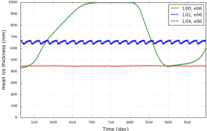
Third, for eccentricities higher than 0.6, the planet is com-pletely frozen around apoastron (corresponding to a mean ice thickness of 1 m, our value of hice.). Figure7shows the evolu-tion of the mean ice thickness for the three different host bod-ies. For an eccentricity of 0.6, the orbital period is 432 days and the planet spends ∼100 days in a completely frozen state, which corresponds to about 20% of its orbital period. When the planet gets closer to periastron, the ice starts melting at a longitude of 60◦ west and liquid water is again available on the dayside around periastron. However, the water vapor concentration be-comes very high and the surface temperature also increases to more than 300 K.
In conclusion, for planets with an eccentricity of less than 0.6, the planet is always able to sustain surface liquid water. The
m ea n i ce th ick n ess (m m ) Time (day)
Fig. 7. Evolution of the mean ice thickness (here a thickness of 1000 mm means the whole planet is covered by the maximum depth of ice allowed in our model: hice= 1 m) of a planet orbiting a 1 L star
(green), a 10−2 L
star (blue), and a 10−4 L star (red) on an orbit of
eccentricity 0.6.
ice-free region changes and shifts as the planet revolves around the star, but it never disappears. For planets with an eccentricity above 0.6, the planet cannot sustain surface liquid water during the whole orbital period. We note that for very high eccentrici-ties and around periastron, the temperatures become higher than the model allows (>400 K). The mean flux approximation is therefore less valid for planets orbiting Sun-like stars on very high eccentricity orbits. However, departing from our definition of habitability based on sea-ice cover, we can only speculate how a potential life form on such a planet would survive this
103 102 101 10-1 100 Pr essu re ( m ba r) 140 160 180 200 220 240 260 280 300 Temperature (K)
Fig. 8.Mean atmospheric temperature profile for planets with an eccen-tricity of 0.4, orbiting a star of 1 L (green), 10−2L (blue), and 10−4L
(red) for periastron and apoastron. We note that the two red curves are superimposed.
succession of frozen winters around apoastron and hot summers around periastron.
5.2. Decreasing the luminosity
Decreasing the luminosity has the effect of decreasing the eccentricity-driven insolation oscillation period. The insolation varies on a shorter timescale and this affects the climate re-sponse. The lower the luminosity, the less time the climate has to respond to the forcing.
5.2.1. Luminosity of L?= 10−2L
For a planet orbiting a 10−2L star with an eccentricity of 0.2, the dayside experiences temperature fluctuations of ∼40 K in about 23 days. It is of the same order of magnitude as for a 1 L star, but the fluctuation happens on a much shorter timescale. We note that decreasing the luminosity was done by decreasing the orbital period (the planets have to be closer to receive a flux of 1366 W/m2), and as the planets are synchronized, the rotation period decreases as well (see Table3). We did not take into ac-count the spectral dependance of the low luminosity stars.
However, the oscillations of the average quantities have a much smaller amplitude than for 1 L . Figure5shows that the amplitudes of oscillations of mean surface temperature and mean ice thickness are significantly damped when decreasing the lumi-nosity from 1 L to 10−2L . Owing to the shorter orbital period, the frequency of the forcing is higher than for the case 1 L and the oscillations in the mean temperature, mean ice thickness, and mean water vapor concentration have a lower amplitude. The cli-mate has indeed less time to react to the insolation forcing.
Figure8shows the mean atmospheric temperature profile for a planet at periastron and apoastron of an orbit of eccentricity 0.4 around the different kinds of object. The difference between apoastron and periastron is important for the case 1 L with a difference of about 40 K at a pressure level of 800 mbar. How-ever, for 10−2L the difference is negligible: a few kelvins from a pressure level of 800 mbar to 50 mbar and in the upper atmo-sphere (pressure<1 mbar). This shows how slowly the climate responds to the higher-frequency forcing.
Decreasing the luminosity has the effect of pushing the limit of liquid water presence toward higher eccentricities. For
Longitude La ti tu de La ti tu de [kg/m2]
Surface ice density
Fig. 9.Surface ice density for a planet of eccentricity 0.8 orbiting a 10−2 L
star. Top graph: when the surface ice density is at its
maxi-mum (just before the periastron passage, i.e., after the long eccentricity-induced winter); bottom graph: when the surface ice density is at its minimum (just after the periastron passage).
example, Figure7 shows that a planet with an eccentricity of 0.6 orbiting a 10−2L star can always sustain surface liquid wa-ter whereas it cannot do so for the whole orbital period if it orbits a 1 L star.
For an eccentricity of 0.8, the planet passes by a complete frozen state around apoastron and partially melts around peri-astron so that for about ten days (∼1/3 of the orbit) there is a small oblong ice-free region. This state is reached in ∼7500 days. Figure9shows the surface ice density on the planet around peri-astron. Just after periastron, less than a percent of the planet’s surface is ice-free at the equator around a longitude of 50◦E (with an extent of about ten degrees in longitude and less than a degree in latitude, see bottom panel of Fig.9). Just before pe-riastron, i.e., after the long eccentricity-induced winter, the re-gion that was ice-free around periastron freezes, but the ice layer depth does not reach its maximum value of 1 m (see top panel of Fig.9). However, for an eccentricity of 0.9, the planet rapidly becomes completely frozen. This state is reached at the first pas-sage at apoastron where the planet freezes completely – 1 m of ice covering the whole planet – and melts partially around pe-riastron. However, even around periastron there is always a thin layer of ice covering the whole planet.
As a result, we find that planets orbiting a 10−2L star can always sustain surface liquid water on the dayside for higher ec-centricities than for a 1 L star (up to 0.8, instead of 0.6). For an eccentricity of 0.8 and higher, the planet remains completely frozen. All in all, the climate simulations are more in agreement with the mean flux approximation for planets orbiting 10−2 L stars. This is due to the averaging of the climate caused by the quicker rotation. However, departing from our definition of hab-itability based on sea-ice cover, we could speculate how a poten-tial life form on such a planet would survive this rapid succes-sion of frozen winters and hot summers (several tens of Kelvins in only ∼20 days).
5.2.2. Luminosity of L?= 10−4L
For an even less luminous host body, the amplitude of the oscil-lations in mean temperature and mean ice thickness are damped with respect to the other cases. As the duration of the year is very short (2 to 4 days, as specified in Table3) there is a more e ffec-tive averaging of the mean surface temperature and ice thickness than for longer orbital period planets. Figure8shows the mean temperature profile for planets at periastron and apoastron of an orbit of eccentricity 0.4. For the case of 10−4L , there is no dif-ference between periastron and apoastron. The shape of the sur-face ice density also changes when the luminosity decreases. For 10−2 L , the ice-free region has a oblong shape, for 10−4 L it has a more peanut shape owing to the passage at periastron. The mean ice thickness for L?= 10−4L is similar to the two previ-ous cases, but does not significantly vary over time (see Fig.7).
We find that planets orbiting a 10−4 L star always remain able to sustain surface liquid water on the dayside throughout the orbit up to very high eccentricities (0.9, instead of 0.8 for 10−2L and 0.6 for 1 L
) owing to the efficient averaging of the climate brought about by the rapid rotation. The mean flux ap-proximation is therefore valid for small luminosities. However, for an eccentricity of 0.8, the dayside temperature varies over ∼50 K, between 300 K and 350 K in less than 4 days. This situa-tion is very extreme for potential life so that the quessitua-tion remains of how life could appear in such an unstable environment.
6. Changing the thermal inertia of the oceans Ioc
and the ice thickness hice
Changing the thermal inertia of the oceans or the ice thickness modifies a few properties of the planets’ climate, but the con-sequences for surface liquid water remain basically the same. The time needed to reach equilibrium does not change signif-icantly when increasing the thermal inertia of the ocean from 18 000 J s−1/2m−2K−1to 36 000 J s−1/2m−2K−1, but – as Fig.10
shows – it increases when increasing the ice thickness from 1 m to 10 m. As the model is allowed to create thicker ice layers, more time is needed to reach the equilibrium ice thickness.
For planets orbiting a 1 L star on a circular orbit, chang-ing the thermal inertia does not influence the overall evolu-tion. The mean surface temperature evolves similarly for ther-mal inertia, and the equilibrium value is slightly higher for Ioc= 18 000 J s−1/2m−2K−1. There is more ice present for Ioc= 18 000 J s−1/2m−2K−1 than for Ioc = 36 000 J s−1/2 m−2 K−1. When increasing the eccentricity, the main difference is that the oscillation amplitude in mean surface temperature and mean ice thickness is lower for Ioc = 36 000 J s−1/2m−2K−1. For an ec-centricity of 0.4, the mean surface temperature fluctuations am-plitude is divided by two when multiplying the thermal inertia by two.
With a higher thermal inertia, the oceans can damp the cli-mate fluctuations more efficiently. Although the temperature fluctuations on the dayside of the planet are still important, the extent of the ocean varies less with Ioc= 36 000 J s−1/2m−2K−1 than with Ioc = 18 000 J s−1/2 m−2 K−1, which makes the en-vironment more stable for potential life. However, this higher thermal inertia of the oceans does not prevent the planet from being completely frozen for very eccentric orbits. For example, for e= 0.8, the planet freezes completely at apoastron.
For planets orbiting a 10−2 L star on a circular orbit, the results are similar to the case 1 L . However, the damping of the oscillation amplitude is not as pronounced. Thanks to the faster rotation of the planet and the more efficient heat redistribution,
Time (day) m ea n i ce th ick n ess (m m ) m ea n su rf ace te m pe ra tu re ( K ) m ea n i ce th ick n ess (m m ) Time (day)
Fig. 10.Mean surface temperature and mean ice thickness of a planet orbiting a 1 L star with an eccentricity of 0.1. Our standard
sce-nario Ioc = 18 000 J s−1/2 m−2 K−1, hice = 1 m is in green;
Ioc = 36 000 J s−1/2 m−2 K−1, hice = 1 m in blue; and Ioc =
18 000 J s−1/2m−2K−1, h
ice= 10 m in red.
the planet climate’s is efficiently averaged and is less sensitive to the difference in thermal inertia.
Increasing the thermal inertia of the ocean allows the cli-mate to have less extreme variations. Following our definition of habitability, changing the thermal inertia of the oceans does not influence the results. While the planet is able to sustain surface liquid water on the dayside for Ioc = 18 000 J s−1/2m−2K−1, it can still do so for Ioc= 36 000 J s−1/2m−2K−1. While the planet is only able to temporarily sustain surface liquid water on the dayside around periastron for Ioc= 18 000 J s−1/2m−2K−1, it is also the case for Ioc= 36 000 J s−1/2m−2K−1.
For planets orbiting a 1 L star on a circular orbit, changing the maximum ice thickness, hice, allowed in the model does not changes the equilibrium temperature of the planet (see Fig.10), the amount of water vapor in the atmosphere, or the geographi-cal repartition ocean-ice. However, more time is needed to reach equilibrium because a thicker ice layer has to be created.
For eccentric orbits, the eccentricity-driven oscillations of mean surface temperature and mean water vapor content are not damped with respect to the case hice = 1 m. However, the shape of the ocean region remains very similar throughout the eccen-tric orbit. The ice layer on the border of the ice-free zone lo-cated in the western and eastern regions, which receives a strong insolation when the planet passes by periastron, only has time to partially melt. The ice-free zone is therefore smaller than for hice = 1 m.
7. Observables
The orbital phase curves of eccentric exoplanets have al-ready been observed (e.g., the close-in giant planets HAT-P-2B
by Lewis et al. 2013, HD 80606 by Laughlin et al. 2009,
and WASP-14b by Wong et al. 2015) and modeled (e.g.,
Iro & Deming 2010; Lewis et al. 2010, 2014; Kane & Gelino
2011; Cowan & Agol 2011; Selsis et al. 2013; Kataria et al.
2013). We show here that the variability caused by the eccen-tricity can be observed by orbital photometry in the visible and in the thermal infrared.
The model computes the top-of-the-atmopshere (TOA) out-going flux in each spectral band and for each of the 64 × 48 columns. The flux received from the planet by a distant ob-server at a distance d in the spectral band∆λ is given by φ∆λ(d)= X lon,lat F∆λ,lon,lat π × Slatµlon,lat d2 ,
where the first term in the sum is the TOA scattered or emitted in-tensity, which is assumed to be isotropic, and the second term is the solid angle subtended by an individual cell; Slatis the area of the cell and µlon,latis the cosine of the angle between the normal to the cell and the direction toward the observer. If this angle is negative then the cell is not on the observable hemisphere of the planet and we set µlon,lat = 0. In practice we use a suite of tools developed bySelsis et al.(2011) that can visualize maps of the emitted/scattered fluxes and produce time- or phase-dependent disk-integrated spectra at the spectral resolution of the GCM.
In addition to the inclination of the system, the orbital lightcurve of an eccentric planet also depends on the orienta-tion of the orbit relative to the observer. Here we consider only observers in the plane of the orbit that see the planet in supe-rior conjunction (full dayside) either at periastron or apoastron. In these configurations, a transit occurs at inferior conjunction and an eclipse at superior conjunction although these events are not included here. As shown by Selsis et al.(2011,2013) and
Maurin et al.(2012), lightcurves are only moderately sensitive to
the inclination between 90◦(transit geometry) and 60◦(the me-dian value). At an inclination of 0◦ (polar observer), the phase angle is constant and the lightcurve is only modulated by the change of orbital distance. In general, the obliquity also intro-duces a seasonal modulation (Gaidos & Williams 2004), but all our cases have a null obliquity. In this article we only describe observables obtained for the 1 L case. The idea is to illustrate the connection between climate and observables rather than to prepare the characterization of Earth-like planets around Sun-like stars as no forthcoming instrument will be able to provide such data. The James Webb Space Telescope (JWST), on the other hand, may be able to obtain (at a large observing-time cost) some data for terrestrial HZ planets around cool host-dwarfs
(Cowan et al. 2015;Triaud et al. 2013;Belu et al. 2013).
How-ever, as before, without accounting for the actual spectral distri-bution of the host, which will be the object of a future study, the generated signatures of planets around M stars and brown dwarfs would not be realistic.
7.1. Circular case
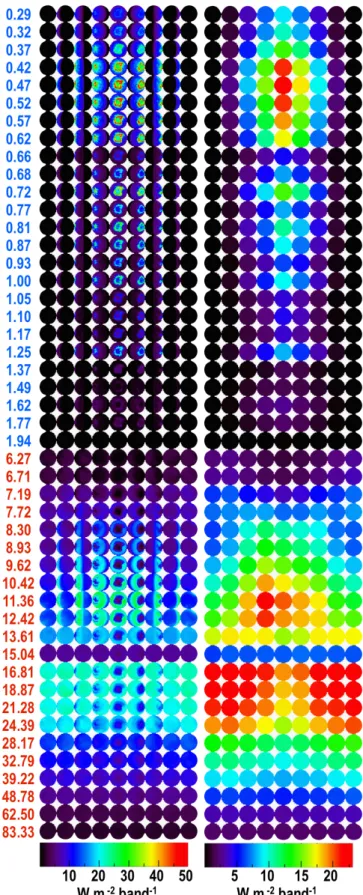
Figure11was obtained for one orbit and a sub-observer point initially located arbitrarily on the equator. Each horizontal line of the plot represents the planet as seen by a distant observer at different orbital phases in a spectral band of the model (only the bands exhibiting a significant flux are shown, hence the gap be-tween 2 and 6 µm). On the left side, the outgoing flux is shown
Fig. 11.Maps of TOA fluxes as seen by a distant observer for one given orbit and one observation geometry (1 L , circular case). Each line
rep-resents one full orbit observed in one band (with the superior conjunc-tion at the center). Each column represents a spectrum of the planet at the GCM resolution at a given orbital phase. The central wavelength of the bands is given in µm on the left. We note the gap between short (scat-tered light, in blue) and long (thermal emission, in red) wavelengths. In the right panel, the averaged spatially unresolved flux is given with a different color scale (owing to a smaller range of values).
15 mm 6.7 mm 11 mm br igh tn ess t em pe ratur e (K ) time/period ecc=0 br igh tn ess t em pe ratur e (K ) time/period ecc=0.2 p a 15 mm 6.7 mm 11 mm p a 15 mm 6.7 mm 11 mm br igh tn ess t em pe ratur e (K ) time/period ecc=0.4
Fig. 12.Thermal phase curves in the 6.7, 11, and 15 µm bands obtained for one orbit, for three eccentricities, and two observation geometries. In the circular case, lightcurves are centered on the superior conjunc-tion (dayside in view) and are time-averaged while the gray area is the 1σ variability due to meteorology. For a given eccentricity, the same orbit is used for both observation geometries. The periastron (p) and apoastron (a) are indicated by vertical lines.
at the spatial resolution of the GCM, while on the right side, the flux is a disk-average. In other words, the line in the right panel is a phase curve, while the column is an instantaneous disk-averaged spectrum. To obtain the flux measured per band at a distance d the value given must be diluted by a factor (R⊕/d)2. In addition to providing both spectral and photometric informa-tion, this type of figure is a useful tool for analyzing the energy budget of the planet: we can see where and at what wavelengths the planet receives its energy and cools to space. For the circular case, the top panel of Fig. 12shows the thermal phase curves and their variability in bands centered on 6.7 µm (H2O absorp-tion), 11 µm (window), and 15 µm (CO2absorption). The phase curve at 0.77 µm (reflected light) and its variability are shown in Fig.13(black curve for the circular case). The long- and short-wave phase curves shown in Figs.11−13present several notice-able features:
− The central region of the dayside, which extends about 40◦ from the substellar point, appears dark in the infrared owing
ecc=0 ecc=0.2 ecc=0.4 pl an et/ star con tr ast ( pp b) time/period
Fig. 13.Reflected-light phase curves in the 0.77 µm band obtained for one orbit, for three eccentricities, and two observation geometries. In the circular case, lightcurves are centered on the superior conjunction (day-side in view) and are time-averaged while the gray area is the 1σ vari-ability due to meteorology. For a given eccentricity, the same orbit is used for both observation geometries, but unlike Fig.12they are shown here with half a period offset so that both are centered on the superior conjunction (vertical line).
to clouds and humidity associated with the massive updraft. At short wavelengths, this substellar cloudy area is instead the most reflective region owing to the scattering by clouds (see Fig.11).
− As the modeled planet has a null obliquity and is locked in a 1:1 spin-orbit resonance, external forcing is constant at any given point on the planet. The three-dimensional structure of the planet that influences the emerging fluxes is not, how-ever, constant. Clouds in particular produce stochastic mete-orological phenomena that induce variations in the observ-ables. The amplitude of this variability is shown in Fig. 13
for one visible band and in Fig.12for three infrared bands probing different levels: the surface (11 µm), the lower and mid-atmospheres (6.7 µm, H2O band), and the upper layers (15 µm, CO2band).
− The CO2 absorption band at 15 µm band is the most notice-able spectral feature, but it exhibits no phase-variation be-cause the atmospheric layers emitting to space in this band (∼50−80 mbar) are efficiently homogenized by circulation. This can be seen in Fig2: the mean day and night thermal profiles are nearly identical in the range 400−20 mbar and clouds (on the dayside) do not extend at altitudes above the 100 mbar layer.
− Most of the cooling occurs within the 9−13 µm atmospheric window, which is transparent down to the surface in the ab-sence of clouds, and between 16 and 24 µm, a domain af-fected by a significant H2O absorption increasing with the wavelength. In the 9−13 µm atmospheric window, most of the emission takes place on the cloud-free ring of the day-side. Except for the cloudy substellar region, the brightness temperature in this window is close to the surface tempera-ture and thus goes from an average of around 270−280 K on the dayside down to 240−250 K on the nightside. In this win-dow, the orbital lightcurve therefore peaks at superior con-junction, as we can see in the top panel of Fig.12.
− At thermal wavelengths absorbed by water vapor (5−7 µm and above 16 µm) most of the emission takes place on the nightside, producing light curves that peak at inferior con-junction. The 6.7 µm and 11 µm lightcurves in the top panel of Fig.12are therefore in phase opposition. On the dayside, the large columns of water vapor result in a high altitude, and therefore a cold, 6.7 µm photosphere (around 200 mbar,
240 K). On the nightside, the 6.7 µm photosphere is the sur-face owing to the low humidity (around 270−280 K).
− Yang et al. (2013) and Gómez-Leal (2013) noted that the
wavelength-integrated emitted and scattered light have op-posite phase variations. We also find this behavior because the emission at λ > 16 µm represents the larger part of the bolometric cooling, as we can see in Fig.11. However, the emission in the 9−13 µm atmospheric band carries a sig-nificant fraction of the bolometric emission and peaks at superior conjunction, as reflected light does. A broadband that includes both spectral regions (9−13 and 16−25 µm) therefore mixes two opposite phase variations, while distin-guishing between these two domains of the thermal emission could provide strong constraints on the nature of the atmo-sphere. Although this should be explored further, these op-posite phase variations between the 9−13 and 16−25 µm in-tervals may be a strong sign of both synchronization and the massive presence of water. Adequate filters at thermal wave-length could be used to exploit this signature while maximiz-ing the signal-to-noise ratio.
7.2. Eccentric cases
The synthetic observables obtained for 1 L and e = 0.2 and e= 0.4 are given in Figs.12(infrared lightcurves),13(reflection lightcurves), and15(full orbital spectro-photometry). Because the maximum eccentricity of an observed possibly rocky planet is only 0.27 (see Sect.1), we choose to show our cases up to an eccentricity of e= 0.4. Several features can be noted:
− The emission in the 15 µm CO2 band remains phase-independent owing to efficient heat redistribution at altitudes above the 100 mb layer. As a consequence, the two obser-vation geometries produce the same lightcurve, which vary only in response to the change of orbital distance (with a lag due to the inertia of the system). This is particularly notice-able in Fig.12.
− The phase opposition that exists in the circular case between the scattered light and the emission in the 8−12 µm atmo-spheric window on the one hand and the emission in the 16−25 µm water vapor window on the other hand disap-pears at e = 0.4 and is hardly seen at e = 0.2 except when the superior conjunction appears at apoastron (second panel in Fig.15). This can be explained by the strong periastron warming that generates a cloudiness that covers a larger frac-tion of the sunlit hemisphere and persists on the nightside. These clouds hence decrease the infrared cooling in the at-mospheric window on the dayside.
− Another effect of this large cloud coverage is to spread the observed scattered light over a broader range of phase an-gles, with no peak at superior conjunction when it occurs at apoastron. This can be seen in Figs.13and15.
7.3. Variation spectrum
The variation spectrum, as defined inSelsis et al.(2011), is the peak amplitude of the phase curve as a function of wavelength. Figure 14shows the minimum and maximum that can be ob-served at any time during a complete orbit for each band of the GCM. Two opposite geometries are presented, for e = 0, 0.2, and 0.4 and L?= L . The difference between the maximum and the minimum gives the amplitude spectrum at the resolution of the GCM. As we only consider cases with a 90◦inclination, the
ecc=0 ecc=0.2 ecc=0.4 m in /m ax of the flu x (W /m /b an d) wavelength (μm) 2 1 10 10-20 10-21 10-20 10-21 10-20 10-21
Fig. 14.Spectral variability. These graphs show, for L?= L and e= 0,
0.2, and 0.4, the maximum and minimum of the flux in each band re-ceived during one orbit. Flux is given at 10 pc. For the reflected light, the minimum is zero as the observer is in the plane of the orbit (in-clination = 90◦
). Superior conjunction occurs at periastron for solid lines and at apoastron for dashed lines. For the circular case (top), solid and dashed lines indicate two arbitrary observer directions separated by 180◦and, in this case, the difference between the two curves is only due
to stochastic meteorological variations.
reflected flux is always null at inferior conjunction (transit). The reflected variation spectrum naturally depends on the eccentric-ity: the closer the planet approaches its hot star, the higher its reflected brightness (for a given albedo). The thermal variation spectrum shows, on the other hand, an overall minor dependency on the eccentricity. The amplitude of the differences in thermal flux increases slightly with eccentricity, but the differences be-tween one eccentricity and another are not significantly higher than those induced by stochastic meteorological changes from one orbit to another. One exception is the amplitude of the vari-ations in the 15 µm band, which increases notably with the ec-centricity from basically no variations at e = 0 to a factor of 2 variation at e= 0.2 and a factor of 5 at e = 0.4.
7.4. Radiative budget
An observer that would have the ability to measure the orbit-averaged broadband emission at short (SW: 0.25−2.0 µm) and/or long (LW: 6−35 µm) wavelengths would be able to estimate the Bond albedo. This could be done with either of these two values