RESEARCH OUTPUTS / RÉSULTATS DE RECHERCHE
Author(s) - Auteur(s) :
Publication date - Date de publication :
Permanent link - Permalien :
Rights / License - Licence de droit d’auteur :
Bibliothèque Universitaire Moretus Plantin
Institutional Repository - Research Portal
Dépôt Institutionnel - Portail de la Recherche
researchportal.unamur.be
University of Namur
Asymptotic behaviour and stability for solutions of a biochemical reactor distributed
parameter model (revised verion)
Dramé, Abdou; Dochain, Denis; Winkin, Joseph
Publication date:
2007
Document Version
Early version, also known as pre-print Link to publication
Citation for pulished version (HARVARD):
Dramé, A, Dochain, D & Winkin, J 2007, Asymptotic behaviour and stability for solutions of a biochemical reactor
distributed parameter model (revised verion)..
General rights
Copyright and moral rights for the publications made accessible in the public portal are retained by the authors and/or other copyright owners and it is a condition of accessing publications that users recognise and abide by the legal requirements associated with these rights. • Users may download and print one copy of any publication from the public portal for the purpose of private study or research. • You may not further distribute the material or use it for any profit-making activity or commercial gain
• You may freely distribute the URL identifying the publication in the public portal ?
Take down policy
If you believe that this document breaches copyright please contact us providing details, and we will remove access to the work immediately and investigate your claim.
FUNDP
Faculté des Sciences Département de Mathématique
Rempart de la Vierge, 8 B-5000 Namur Belgique
Asymptotic behaviour and stability for solutions of a
biochemical reactor distributed parameter model
(revised version)
A.K. DRAME, D. DOCHAIN andJ. J. WINKIN Report 2007/06
P
UBLICATIONS DU
D
EPARTEMENT DE
M
ATHEMATIQUE
Asymptotic behaviour and stability for solutions
of a biochemical reactor distributed parameter
model
A. K. Dram´e, D. Dochain, and J. J. Winkin,
Abstract
This paper deals with the dynamical analysis of a tubular biochemical reactor. The existence of nonnegative state trajectories and the invariance of the set of all physically feasible state values under the dynamical equation as well as the convergence of the state trajectories to equilibrium profiles are proved. In addition, the existence of multiple equilibrium profiles is analyzed. It is proved that under physically meaningful conditions the system has two stable and one unstable equilibrium profiles.
Index Terms
state trajectories, asymptotic behaviour, multiple equilibrium profiles, stability, biochemical reactor.
I. INTRODUCTION
The dynamical analysis and control of tubular biochemical reactors have motivated many research activities over the last decades ([5], [6], [11], [13], [24], etc.). The dynamics of these reactors are described by distributed parameter systems and typically by nonlinear partial differential equations with e.g. Danckwerts type boundary conditions, see e.g. [5], [6]. The aim of this paper is to analyze the dynamical nonlinear model of a fixed bed tubular biochemical reactor with axial dispersion. The nonlinearity in the model arises from the substrate inhibition term in the model equations and is a specific rational function of the state components. The basis of the model under study is derived from the work performed on anaerobic digestion in the pilot fixed bed reactor of the LBE-INRA in Narbonne (France) and is mainly inspired from the dynamical models built and validated on the process ([3], [21]). This study follows the preliminary one performed in [13].
The existence and uniqueness of the state trajectories (limiting substrate and limiting biomass) as well as their asymptotic behaviour are analyzed for this model. First of all, it is proved that the trajectories exist on the whole (nonnegative real) time axis and the set of all physically feasible state values is invariant under the dynamical equation. This set takes into account the positivity of the state variables as well as a saturation condition on the substrate. Second, the asymptotic behaviour of the trajectories is investigated and it is proved that the trajectories converge to equilibrium solutions of the system.
In addition the existence of multiple equilibrium profiles is analyzed. The multiplicity is established together with the stability of equilibrium profiles by using phase plane analysis of ordinary differential equations.
The paper is organized as follows : in Section 2, the dynamical model is presented and some preliminary analysis is performed. In Section 3, the state trajectories of the tubular biochemical reactor dynamical model are analyzed. Sections 4 and 5 deal with the existence of multiple equilibrium profiles and their stability. Finally, some concluding remarks are given in Section 6.
II. THE DYNAMICAL MODEL
Applying the mass balance principles to the limiting substrate concentration S(τ, ζ) and the living biomass concentration X(τ, ζ) leads to the following nonlinear system of partial differential equations :
∂S ∂τ = D ∂2S ∂ζ2 − ν ∂S ∂ζ − kµ(S, X)X (II.1) ∂X ∂τ = −kdX + µ(S, X)X, (II.2)
with the boundary conditions : for all τ ≥ 0,
D∂S
∂ζ(τ, 0) − νS(τ, 0) + νSin= 0 and
∂S
∂ζ(τ, L) = 0. (II.3)
Paper submitted to IEEE Transactions on Automatic Control.
A. K. Dram´e and D. Dochain are with the Universit´e catholique de Louvain, CESAME, 4-6 av. G. Lematre, B-1348 Louvain-La-Neuve, Belgium, [email protected], [email protected]
J. J. Winkin is with the University of Namur (FUNDP), Department of Mathematics, 8 Rempart de la Vierge, B-5000 Namur, Belgium, [email protected]
The substrate inhibition is expressed via the following law :
µ(S, X) = µ0
S
KSX + S +K1iS2
. (II.4)
In the equations above, D, k, kd, KS, Ki, Sin, ν and µ0 are positive parameters. In particular, D, ν and kd denote the
axial dispersion coeficient, the superficial fluid velocity and the kinetic constant, respectively. The parameters k and KS are
dimensionless, whereas Kihas the dimension of a concentration. In addition the specific growth rate µ(S, X) has the dimension
of the inverse of a time. Finally ζ ∈ [0, L] and τ ≥ 0 denote the spatial and time variables, respectively, and L denotes the
length of the reactor.
Observe that the reaction considered here is autocatalytic, i.e. the biomass is not only a product of the reaction, but also a catalyst of that reaction. This feature is modelled by the last term in the right-hand sides (RHS) of equations (II.1) and (II.2). In addition the two first terms of the RHS of equation (II.1) are diffusion and convection terms, respectively. The removal-mortality phenomenon for the biomass is modelled by the first term of the RHS of equation (II.2). This corresponds to the observation that biomass aggregates reach a maximum size beyond which solid particles leave the reactor : this happens notably because of shear forces between the fluid (substrate) going through the reactor and the solid (biomass). The selection of the above model is largely motivated by its analogy with the single microbial growth model with Haldane kinetics in perfectly mixed reactors, for which the existence of multiple (stable and unstable) equilibria have been emphasized (see e.g. [1], [2], [4], [19]). From a physical point of view, it is expected that the following saturation condition holds :
0 ≤ S ≤ Sin, (II.5)
where Sin is the inlet limiting substrate concentration. One of the contributions of this paper is to prove that the physiscal
set defined by inequalities (II.5) is invariant under the dynamic equation of the biochemical reactor model introduced above. As usual, the dynamical analysis of this model will be performed on an equivalent dimensionless infinite dimensional system description. By using the new state components
˜x1:= Sin− S Sin and ˜x2:= X Sin
and the new spatial and time variables
z := ζ
L and t :=
ν Lτ, respectively, the model (II.1)-(II.2) can be rewritten as the following two PDE’s :
∂ ˜x1 ∂t = 1 Pe ∂2˜x 1 ∂z2 − ∂ ˜x1 ∂z + k˜µ(˜x1, ˜x2)˜x2 (II.6) ∂ ˜x2 ∂t = −γ˜x2+ ˜µ(˜x1, ˜x2)˜x2, (II.7)
with the boundary conditions : for all t≥ 0,
1 Pe ∂ ˜x1 ∂z (t, 0) − ˜x1(t, 0) = 0 and ∂ ˜x1 ∂z (t, 1) = 0. (II.8)
where the modified substrate inhibition law ˜µ(˜x1, ˜x2) is given by
˜µ = β (1 − ˜x1)
KS˜x2+ (1 − ˜x1) + α(1 − ˜x1)2
, (II.9)
and where the constants α, β, γ and Pe (Peclet number) are given respectively by
α := Sin Ki , β := L νµ0, γ := L νkd and Pe:= νL D,
respectively. We also introduce the following change of variables in order to transform the equation (II.6)-(II.8) into a reaction-diffusion equation with a bounded perturbation. This transformation is for mathematical analysis purpose and we will use the resulting reaction-diffusion type equation to study asymptotic behaviour of solution of the system (II.6)-(II.8). This is a one-to-one transformation, so the two systems are equivalent.
x1(z) := e−
Pe
2z˜x1(z) and x2(z) := e−Pe2z˜x2(z) for all z ∈ [0, 1], for all ˜x1, ˜x2∈ C[0, 1].
Then, we have the following equations : ∂x1 ∂t = 1 Pe ∂2x 1 ∂z2 − Pe 4 x1+ k˜˜µ(x1, x2)x2 (II.10)
∂x2
∂t = −γx2+ ˜˜µ(x1, x2)x2, (II.11)
with the boundary conditions : for all t≥ 0,
∂x1 ∂z (t, 0) = Pe 2 x1(t, 0) and ∂x1 ∂z (t, 1) = − Pe 2 x1(t, 1), (II.12) where ˜˜µ(z, x1, x2) = ˜µ(e Pe 2 zx1, ePe2 zx2).
Now the dimensionless model (II.10)-(II.12) can be given an infinite dimensional state space description as follows. Consider
the Banach space C[0, 1] (equipped with the usual norm%.%C0) on which we define the unbounded linear operator A1 by :
D(A1) = {x1∈ C2[0, 1] : dx1 dz (0) − Pe 2 x1(0) = 0, dx1 dz (1) + Pe 2 x1(1) = 0}, A1x1= 1 Pe d2x 1 dz2 − Pe 4 x1, ∀ x1∈ D(A1).
We also consider the bounded linear operator A2 = −γI where I is the identity operator on C[0, 1]. Therefore equations
(II.10)-(II.12) can be rewritten as follows : for all t≥ 0, dx(t)
dt = Ax(t) + N(x(t)),
where x := (x1, x2)T is a vector of the Banach space Z := C[0, 1]⊕ C[0, 1] endowed with the natural norm %.%Z =
%.%C0+ %.%C0, A := diag(A1, A2) is defined on its domain D(A) = D(A1) ⊕ C[0, 1] and N is the nonlinear operator defined
on X by N (x) := (N1(x), N2(x)) where
N1= kN2 and N2(x1, x2) = ˜˜µ(x1, x2)x2.
By the arguments given in [7], the operator A1 is the infinitesimal generator of an exponentially stable C0-semigroup of
bounded linear operators T1(t) on C[0, 1]. It is easy to see that A2 is the infinitesimal generator of an exponentially stable C0
-semigroup of bounded linear operators T2(t) = e−γtI on C[0, 1]. Therefore A is the infinitesimal generator of an exponentially
stable C0-semigroup of bounded linear operators T (t) on Z given by T (t) = diag(T1(t), T2(t)). Moreover, the semigroups
T1(t) and T2(t) are analytic in C[0, 1] and T1(t) is compact in C1[0, 1]. Therefore, T (t) is analytic in Z.
III. STATE TRAJECTORIES
A. Global existence
The well-posedness and invariance properties of the state trajectories of the biochemical reactor dimensionless model (II.10)-(II.12) are now studied by using the description of an abstract semilinear Cauchy Problem of the form
dx(t) dt = Ax(t) + N(x(t)), x(0) = x0∈ Ω, (III.1) where the operators A and N are defined in the previous section and Ω, motivated by (II.5), is the physically admissible set given by :
Ω = {(x1, x2) ∈ Z : 0 ≤ x1(z) ≤ e−
Pe
2 z, 0 ≤ x2(z) for all z∈ [0, 1]} (III.2)
The main tool used in the analysis of this problem is the following theorem, which is an equivalent version of Theorem 5.1 of [16, p.355]. This Theorem gives sufficient conditions for the existence and the uniqueness of the mild solution of equations
of type (III.1) on the whole interval [0, +∞) and for the invariance of the set Ω under the dynamical equations.
Theorem 3.1: [16, p. 355, Theorem 5.1] Let (X,%.%) be a real Banach space and ˜T (t) a C0-semigroup of bounded linear
operators such that % ˜T (t)% ≤ Meδt, for all t
≥ 0, for some δ ∈ R and M ≥ 1. Let ˜A be the infinitesimal generator of ˜T (t)
and ˜D be a closed subset of X. Assume also that ˜N is a continuous function from ˜D into X. Let us consider the following
initial value problem
dx(t) dt = ˜Ax(t) + ˜N (x(t)), x(0) = x0∈ ˜D. (III.3) Assume that
(ii) For all x∈ ˜D,
lim
h→0+
1
hd(x + h ˜N (x); ˜D) = 0;
(iii) ˜N is continuous on ˜D and there exists lN˜ ∈ R+ such that the operator ( ˜N− lN˜I) is dissipative on ˜D.
Then for all x0 ∈ ˜D, (III.3) has a unique mild solution x(t, x0) on [0,,∞[. Moreover, if T(t) is defined on ˜D by T(t)x0=
x(t, x0), for all t ≥ 0 and x0∈ ˜D, it is a nonlinear semigroup on ˜D, with ( ˜A + ˜N ) as its generator.
The following lemma holds.
Lemma 3.2: The semigroup T (t) is positive and for all t≥ 0, T (t)Ω ⊂ Ω.
Proof : Let x0= (x0,1, x0,2) ∈ Ω and x(t) = T (t)x0= (T1(t)x0,1, T2(t)x0,2)T, for t≥ 0. Obviously, x2(t) = T2(t)x0,2 ≥ 0,
for all t≥ 0. We have to prove that 0 ≤ x1(t, z) = (T1(t)x0,1) (z) ≤ e−
Pe
2z, for all t ≥ 0 and z ∈ [0, 1]. Let us introduce
y1(t) := −x1(t) for all t ≥ 0. Since the semigroup T1(t) is analytic in C[0, 1], then y1 satisfies the equation
∂y1 ∂t = 1 Pe ∂2y 1 ∂z2 − Pe 4 y1, y1(0) = −x0,1, ∂y1 ∂z (t, 0) = Pe 2 y1(t, 0) and ∂y1 ∂z (t, 1) = − Pe 2 y1(t, 1).
It follows by the comparison theorem (see eg. [20, Chap 3, Theorem 8]) that y1 reaches its maximum at a boundary point
(0, z), z ∈]0, 1[, (t, 0), t > 0 or (t, 1), t > 0. If this maximum is reached at (t, 0) (resp. at (t, 1)), then it follows from [20, Chap 3, Theorem 8] that
∂y1
∂z(t, 0) < 0 (resp. ∂y1
∂z (t, 1) > 0).
Hence, considering the boundary conditions, the solution y1 cannot have a positive maximum at (t, 0) and (t, 1). It follows
that its maximum is negative and therefore 0≤ x1(t), for all t ≥ 0. Since T1(t) is a semigroup of contraction,
x1(t, z) ≤ %x1(t)%C0 ≤ %x0,1%C0 ≤ e−
Pe
2 z, for all z∈ [0, 1] and t ≥ 0.
It follows that T (t)x0∈ Ω that is : the semigroup T (t) is positive and Ω is invariant under T (t). !
Remark 3.1: It is easy to see that the function N : Ω−→ Z is Lipschitz continuous and that its Lipschitz constant, lN, can
be obtained by rather simple calculations.
Now let Λ be a closed interval ofR and consider the set
K(Λ, C[0, 1]) :={φ ∈ C[0, 1] : φ(z) ∈ Λ for all z ∈ [0, 1]}.
The proof of the following Lemma is similar to the one of [11, Proposition 3.1] is therefore omitted.
Lemma 3.3: Assume that Λ = [a, b], fc : Λ −→ R is a continuous function and fp : [0, 1] × Λ −→ R is a nonnegative
bounded measurable function. If fc(a) ≥ 0 and fc(b) ≤ 0, then
lim
h→0+
1
hd(φ + hB(φ), K(Λ, C[0, 1])) = 0,
where the substitution operator B is defined on K(Λ, C[0, 1]) by
[B(φ)](z) := fp(z, φ(z)).fc(φ(z)),
for all z∈ [0, 1], for all φ ∈ K(Λ, C[0, 1]).
Remark 3.2: By replacing [a, b] by [a, ∞) in Lemma 3.3 the conclusion holds if only the condition fc(a) ≥ 0 is satisfied.
The following Lemma can be deduced from Lemma 3.3 and Remark 3.2.
Lemma 3.4: For all (x1, x2) ∈ Ω,
lim
h→0+
1
hd((x1, x2) + hN((x1, x2)); Ω) = 0.
Finally, we can deduce from Remark 3.1 that the operator N− lN is dissipative on Ω, where lN is the Lipschitz constant of
N .
In the following theorem, the global existence of state trajectories is reported. It follows from the Lemmas above and Remark 3.1, by using Theorem 3.1.
Theorem 3.5: For every x0 ∈ Ω, equation (III.1) has a unique mild solution x(t, x0) on the interval [0, +∞[. Moreover,
if one sets T(t)x := x(t, x0) then, (T(t))t≥0 is a strongly continuous nonlinear semigroup on Ω, generated by the operator
A + N .
Hence the state trajectories of the tubular biochemical reactor nonlinear model given by (III.1) (or equivalently (II.10)-(II.12))
are well-defined on the whole time interval [0, +∞). Moreover, the physically feasible set Ω is invariant under this model
dynamics, i.e. for all t≥ 0, T(t)Ω ⊂ Ω.
B. Asymptotic behaviour
This subsection deals with the asymptotic behaviour of solutions of (III.1). The main result is the convergence of the solutions to equilibrium profiles of the dynamical model of the tubular biochemical reactor. We will successively give some regularity and relative compactness result of the solutions before dealing with their asymptotic behaviour. For the sake of simplicity, we
shall denote by x(t) the solution x(t, x0) of (III.1). The proof of following Lemma is similar to the one of [7, Lemma 3.1]
and is therefore omitted.
Lemma 3.6: (i) For any x0∈ Ω, the mild solution x(t) of (III.1) is a classical solution, i.e. :
x∈ C([0, +∞[; Z) ∩ C1(]0, +∞[; Z),
x(t)∈ D(A), for all t > 0 and x(t) satisfies (III.1) in the usual sense. (ii) For any t0> 0, the subsets
{Ax(t), t ≥ t0} and {
∂x(t)
∂t , t≥ 0}
are bounded in Z. Moreover, the norms of C[0, 1] and C1[0, 1] are equivalent on the subset {x
1(t), t ≥ t0} ; i.e.
∃ M0> 0 /∀ t ≥ t0, %x1(t)%C0 ≤ %x1(t)%C1 ≤ M0%x1(t)%C0.
In view of Lemma 3.6, we shall understand by solution of (III.1) a global classical solution.
Let us define now the following functionals, keeping in mind the idea of some kind of energy function. J1(x1, x2) = % 1 0 & 1 2Pe ' ∂x1 ∂z (2 − % x1 0 F1(z, u, x2)du ) dz + 1 4(x21(0) + x21(1)), J2(x1, x2) = − % 1 0 % x2 0 F2(z, x1, u)dudz, where F1(z, x1, x2) = −Pe 4 x1+ k˜˜µ(z, x1, x2)x2 and F2(z, x1, x2) = −γx2+ ˜˜µ(z, x1, x2)x2. We finally define J(x1, x2) = J1(x1, x2) + J2(x1, x2).
The functional J is well defined along the trajectories of equation (III.1) and the following statement holds.
Lemma 3.7: For any solution x(t) of (III.1), we have
d dtJ(x(t)) = − % 1 0 &' ∂x1 ∂t (2 +'∂x2 ∂t (2) dz − % 1 0 &% x1(t,z) 0 ∂ ∂t(F1(z, u, x2(t, z)))du + % x2(t,z) 0 ∂ ∂t(F2(z, x1(t, z), u))du ) dz.
Proof : Let x(t) = (x1(t), x2(t)) be a solution of (III.1), then the component x1(t) satisfies the equation
∂x1 ∂t = 1 Pe ∂2x 1 ∂z2 − Pe 4 x1+ N1(x1(t), x2(t)), ∂x1 ∂z(t, 0) = Pe 2 x1(t, 0), ∂x1 ∂z (t, 1) = Pe 2 x1(t, 1).
By differentiating this equation with respect to t and by using the comparison theorem [20, Chap 3, Theorem 8], one can prove that ∂x1
∂t(t) belongs to C
1[0, 1] for all t > 0. The following calculation is then well founded.
d dtJ1(x(t)) = % 1 0 & 1 2Pe ∂ ∂t ' ∂x1 ∂z (2 − F1(z, x1, x2)∂x1 ∂t − % x1(t,z) 0 ∂ ∂t(F1(z, u, x2(t, z)))du ) dz +1 4 ∂ ∂t(x 2 1(t, 0) + x21(t, 1)) =% 1 0 & 1 Pe ∂x1 ∂z ∂ ∂t '∂x 1 ∂z ( − F1(z, x1, x2) ∂x1 ∂t − % x1(t,z) 0 ∂ ∂t(F1(z, u, x2(t, z)))du ) dz +1 4 ∂ ∂t(x 2 1(t, 0) + x21(t, 1)) = −% 1 0 ' 1 Pe ∂2x 1 ∂z2 + F1(z, x1, x2) (∂x 1 ∂t dz− % 1 0 % x1(t,z) 0 ∂ ∂t(F1(z, u, x2(t, z)))dudz + 1 Pe ' ∂x1 ∂t ∂x1 ∂z |z=1− ∂x1 ∂t ∂x1 ∂z |z=0 ( +1 4 ∂ ∂t(x 2 1(t, 0) + x21(t, 1)).
Using the boundary conditions in (II.12) and the fact that x1(t) satisfies the PDE above, it follows that
d dtJ1(x(t)) = − % 1 0 ' ∂x1 ∂t (2 dz− % 1 0 % x1(t,z) 0 ∂ ∂t(F1(z, u, x2(t, z)))dudz. On the other hand,
d dtJ2(x(t)) = − % 1 0 &' ∂x2 ∂t (2 − % x2(t,z) 0 ∂ ∂t(F2(z, x1(t, z), u))du ) dz. Hence d dtJ(x(t)) = − % 1 0 &' ∂x1 ∂t (2 +'∂x2 ∂t (2) dz − % 1 0 &% x1(t,z) 0 ∂ ∂t(F1(z, u, x2(t, z)))du + % x2(t,z) 0 ∂ ∂t(F2(z, x1(t, z), u))du ) dz. !
Let us denote by K(τ ), for any τ ≥ 0, the subset of Z given by
K(τ ) ={x(t), t ≥ τ}.
The following Lemma states a relative compactness of the solutions of (III.1). Note that the invariance of the set Ω implies the boundedness of solutions of (III.1). Note also that N2 is Lipschitz continuous in C[0, 1] with constant lN2.
Lemma 3.8: Assume that lN2< γ and let x0= (x0,1, x0,2) ∈ Ω and x(t) be the solution of (III.1), then K(0) is relatively
compact in Z. Moreover, for any t0> 0, K(t0) is relatively compact in C1[0, 1] ⊕ C[0, 1].
Proof : 1. Relative compactness in Z
Observe that x1(t) satisfies the integral equation
x1(t) = T1(t)x0,1+
% t
0
T1(t − s)N1(x1(s), x2(s))ds
and recall that the semigroup T1(t) is compact in C[0, 1] and N1(x1(t), x2(t)) is bounded in C[0, 1]. Then, it follows from
[18, p. 236, Lemma 2.4] that x1(t) has a compact closure in C[0, 1].
Let us now prove that x2(t) is relatively compact in C[0, 1] by applying Ascoli-Arzela’s Theorem. To apply this Theorem, it
Let z0, z∈ [0, 1], we have x2(t)(z0) − x2(t)(z) = (T2(t)x0,2)(z0) − (T2(t)x0,2)(z) + % t 0 (T2(t − s)N2(x1(s), x2(s)))(z0) − (T2(t − s)N2(x1(s), x2(s)))(z)ds = e−γt(x 0,2(z0) − x0,2(z)) + % t 0 e−γ(t−s)(N2(x1(s), x2(s)))(z0) − N2(x1(s), x2(s)))(z)) ds.
Since N2 is Lipschitz continuous with constant lN2, we have
|x2(t)(z0) − x2(t)(z)| ≤ e−γt|x0,2(z0) − x0,2(z)|
+ lN2
% t 0
e−γ(t−s)(|x1(s)(z0) − x1(s)(z)| + |x2(s)(z0) − x2(s)(z)|) ds.
Let ε > 0. Since x1(t) is relatively compact in C[0, 1] then, there exists δ0> 0 such that
|z − z0| ≤ δ0=⇒ |x1(s)(z0) − x1(s)(z)| < ε, ∀ s ≥ 0.
Then, for z∈ [0, 1] satisfying |z − z0| ≤ δ0, we have
eγt |x2(t)(z0) − x2(t)(z)| ≤ (1 + lN2 γ )εe γt+ l N2 % t 0 eγs |x2(s)(z0) − x2(s)(z)|ds.
By applying Gronwall’s inequality, we have eγt|x 2(t)(z0) − x2(t)(z)| ≤ (1 +lN2 γ )εe γt+ l N2(1 + lN2 γ )ε % t 0 elN2(t−s)eγsds ≤ (1 +lNγ2)εeγt+lN2(1 + lN2 γ ) γ− lN2 εelN2te(γ−lN2)t ≤ γ(1 + lN2 γ )e γt γ− lN2 ε. So, as lN2 < γ, let ε0 be such that
ε = γ− lN2
γ(1 +lN2
γ )
ε0.
By using ε0 in the role of ε in the previous calculations, we find that for z∈ [0, 1]
|z − z0| ≤ δ0=⇒ |x2(t)(z) − x2(t)(z0)| < ε, ∀ t ≥ 0.
It follows that x2(t) is equicontinuous in C[0, 1] and by Ascoli-Arzela’s Theorem, x2(t) has compact closure in C[0, 1].
2. Relative compactness in C1[0, 1] ⊕ C[0,
,1]
By Lemma 3.6, the setK0= {x1(t), t ≥ t0} is bounded in C1[0, 1]. Observe also that for each z ∈ [0, 1], {x1(t, z)), t ≥ t0}
has a compact closure inR. Once again, by Lemma 3.6, the norms of C[0, 1] and C1[0, 1] are equivalent on K
0. Since x1(t)
is equicontinuous in C[0, 1] thenK0is also equicontinuous in C1[0, 1]. It follows from Ascoli-Arzela’s Theorem that K(t0)
has a compact closure in C1[0, 1] ⊕ C[0, 1]. This completes the proof. !
As the solutions of (III.1) are defined for all time, we can define their ω-limit in the usual way as for dynamical systems.
Definition 3.1: The ω-limit set of a solution x(t) of (III.1) with respect to the topology of Z is the set defined by
ω(x0/Z) ={ϕ ∈ Z : ∃(tn)n∈N, tn −→
n→+∞+∞ and x(tn) −→n→+∞ϕ in Z}.
Lemma 3.9: Let x(t) = (x1(t), x2(t)) be a solution of (III.1). Then, the ω-limit set of x(t) with respect to the topology of
Z coincides with its ω-limit set with respect to the topology of C1[0, 1] ⊕ C[0, 1] ; i.e.
ω(x0/Z) = ω(x0/C1[0, 1] ⊕ C[0, 1]).
Proof : Observe that
ω(x0/C1[0, 1] ⊕ C[0, 1]) = ω(x01/C1[0, 1]) ⊕ ω(x02/C[0, 1]).
We have only to prove the identity for the component x1(t) of x(t). Obviously,
ω(x0,1/C1[0, 1]) ⊂ ω(x0,1/C[0, 1]).
Let ϕ∈ ω(x0,1/C[0, 1]), then there exists (tn)n∈N such that
tn −→
n→+∞+∞ and x1(tn) −→n→+∞ϕ in C[0, 1].
Without loss of generality, we can assume that (tn)n≥0 is increasing and that t0 > 0. From Lemma 3.8, x1(t) is eventually
relatively compact in C1[0, 1]. Then there exists a subsequence (t
nk)k≥0 of (tn)n≥0 and a function ˜ϕ∈ C
1[0, 1] such that
tnk −→
k→+∞+∞ and x1(tnk) −→k→+∞ϕ˜ in C 1[0, 1].
It follows from the uniqueness of the limit in C[0, 1] that ϕ = ˜ϕ and ϕ∈ C1[0, 1], since the above convergence also holds
in C[0, 1]. Hence
ω(x0,1/C[0, 1])⊂ ω(x0,1/C1[0, 1]).
This completes the proof. !
In view of this Lemma, the ω-limit set of a solution x(t) will be simply denoted by ω(x0).
The following Theorem is one of the main results related to the asymptotic behaviour of solutions of (III.1) established here.
Theorem 3.10: Assume that lN2 < γ and let x0 = (x0,1, x0,2) ∈ Ω and x(t) be the solution of (III.1) with x(0) = x0 and
ω(x0) its ω-limit set. Then ω(x0) is non empty and is contained in D(A). Moreover ω(x0) consists of equilibrium profiles of
(III.1).
Proof : Let x0 ∈ Ω, from Lemma 3.8, ω(x0) is non empty. Therefore, there exist ϕ ∈ ω(x0) and a sequence (tn)n≥0 such
that
tn −→
n→+∞+∞ and x(tn) −→n→+∞ϕ in Z.
Let us introduce ¯xn := x(tn) and ¯yn(t) := x(t + tn) for all n ∈ N and t ≥ 0. Then, ¯yn(t) satisfies the integral equation
¯yn(t) = T (t)¯xn+
% t
0
T (t− s)N(¯yn(s))ds. (III.4)
Recall that T (t) is a C0-semigroup of contractions and N is Lipschitz continuous with constant lN. Then,
%¯yn(t) − ¯ym(t)%Z≤ %¯xn− ¯xm%Z+ lN
% t
0 %¯y
n(s) − ¯ym(s)%Zds, for all t≥ 0 and n, m ∈ N.
Hence, by using Gronwall’s inequality : for any t0> 0, there exists a constant C > 0 such that
sup
0≤t≤t0%¯y
n(t) − ¯ym(t)%Z ≤ C%¯xn− ¯xm%Z, ∀ m, n ∈ N.
Then considered as a subset of C([0, t0]; Z), (¯yn)n≥0is a Cauchy sequence. It follows that there exists a continuous function
y : [0,∞[−→ Z such that
∀ t0> 0, lim n→∞0≤t≤tsup0
%¯yn(t) − y(t)%Z = 0.
Taking the limit in (III.4) when n→ ∞, leads to
y(t) = T (t)ϕ +
% t
0
T (t− s)N(y(s))ds, for all t ≥ 0.
Then y(t) is a mild solution of (III.1) and by Lemma 3.6, y(t) is a classical solution of (III.1).
Moreover, ¯yn(t) ∈ D(A) and AT (t) ∈ L(Z) for all t ≥ 0 and n ∈ N, and
A¯yn(t) = AT (t)¯xn+
% t
0
Taking the limit, when n→ ∞, lim n→∞A¯yn(t) = AT (t)ϕ + % t 0 AT (t− s)N(y(s))ds = Ay(t).
Since the function N is continuous, one has
lim n→∞ d¯yn dt (t) = dy(t) dt .
By Lemma 3.7, for any t0> 0
J(x(t0)) − J(x(t)) = % t t0 % 1 0 &' ∂x1 ∂τ (2 +'∂x2 ∂τ (2) dzdτ − % t t0 % 1 0 &% x1(τ,z) 0 ∂ ∂τ (F1(z, u, x2(τ, z))) du + % x2(τ,z) 0 ∂ ∂τ (F2(z, x1(τ, z), u)) du ) dzdτ.
As x(t) is bounded in Z (there exists M0 such that 0≤ %x(t)%Z ≤ M0, for all t≥ 0), we define the functions
G1(z, τ, u) = F1(z, u, x2(τ, z)), if 0 ≤ u ≤ x1(τ, z) 0 if u≥ x1(τ, z) G2(z, s, u) = F2(z, x1(τ, z), u), if 0 ≤ u ≤ x2(τ, z) 0 if u≥ x2(τ, z) Then, % t t0 % x1(τ,z) 0 ∂ ∂τ(F1(z, u, x2(τ, z)))dudτ = % t t0 % M0 0 ∂ ∂τ(G1(z, τ, u))dudτ = % M0 0 % t t0 ∂ ∂τ(G1(z, τ, u))dudτ = % M0 0 (G1(z, t, u) − G1(z, t0, u)) du = % x1(t,z) 0 (F1(z, u, x2(t)) − F1(z, u, x2(t0))) du.
As x1(t) is bounded and F1 is continuous, then the integral
% 1 0 % t t0 % x1(τ,z) 0 ∂ ∂τ(F1(z, u, x2(τ, z)))dudτdz, t ≥ t0 is bounded.
Similarly, by using G2, we show that the integral
% 1 0 % t t0 % x1(τ,z) 0 ∂ ∂τ(F2(z, x1(τ, z), u))dudτdz, t ≥ t0 is bounded.
By Lemma 3.6, J(x(t)) is bounded in Z. Hence,
% ∞ t0 % 1 0 &'∂x 1 ∂τ (2 +'∂x2 ∂τ (2) dzdτ <∞. Taking any 0 < t0< t1<∞, one gets the following identity
lim n→∞ % t1 t0 % 1 0 &' ∂ ¯yn,1 ∂t (2 +'∂ ¯yn,2 ∂t (2) dzdt = lim n→∞ % t1+tn t0+tn % 1 0 &' ∂x1 ∂t (2 +'∂x2 ∂t (2) dzdt = 0. It follows that % t1 t0 % 1 0 &' ∂y1 ∂t (2 +'∂y2 ∂t (2) dzdt = 0.
Hence, y is independent of t and y(t) = ϕ, for all t≥ 0. y(t) being a classical solution of (III.1), it follows that
ϕ∈ D(A) and Aϕ + N(ϕ) = 0.
! The convergence of solutions of (III.1) to its equilibrium profiles is reported now.
Theorem 3.11: Asssume that lN1 < γ and let x0 = (x0,1, x0,2) ∈ Ω and x(t) be the solution of (III.1) with x(0) = x0.
Then there exists an equilibrium profile ¯x of (III.1) such that lim
t→∞x(t) = ¯x in C
1[0, 1] ⊕ C[0, 1].
Proof : Let x(t) = (x1(t), x2(t)) be the solution of (III.1) and ω(x0) its ω-limit set. Let us define
f (t, z, w) = N1(w, x2(t, z)),
Then, the x1-equation in (III.1) can be written as follows
∂x1 ∂t = 1 Pe ∂2x 1 ∂z2 − Pe 4 x1+ f(t, z, x1) x1(0, z) = x0,1(z) ∂x1 ∂z (t, 0) = Pe 2 x1(t, 0); ∂x1 ∂z (t, 1) = − Pe 2 x1(t, 1), (III.5)
and we denote by ω(x0,1) its ω-limit set, that is : ω(x0) = ω(x0,1) ⊕ ω(x0,2). By Theorem 3.10, ω(x0) consists of equilibrium
solutions. Then, ω(x0,1) consists of solutions of ordinary differential equations and the convergence of subsequences of x1(t)
holds in norm C1[0, 1]. Then, by Theorem A in [14], ω(x
0,1) contains at most one element ¯x1. As ω(x0,1) is non empty, then
it contains exactly one element. It follows that x1(t) converges towards ¯x1in norm C1[0, 1]. Therefore, x1(t), x2(t) converges
to an equilibrium (¯x1, ¯x2) in C1[0, 1] ⊕ C[0, 1]. !
IV. MULTIPLE EQUILIBRIUM PROFILES
In this section, the equilibrium profiles analysis of the biochemical reactor dimensionless model (II.6)-(II.9) is performed by using a perturbation theory. The equilibrium profiles (¯x1, ¯x2) are solutions of
1 Pe ¯x!! 1− ¯x ! 1+ k˜µ(¯x1, ¯x2)¯x2 = 0, −γ ¯x2+ ˜µ(¯x1, ¯x2)¯x2 = 0, 1 Pe ¯x! 1(0) − ¯x1(0) = ¯x ! 1(1) = 0. (IV.1)
Obviously, the system (IV.1) has a trivial solution (¯x1, ¯x2) = (0, 0) which corresponds to the reactor washout ( ¯S, ¯X) =
(Sin, 0) when considering the initial state variables. In the following, we shall be interested in solution of (IV.1) which satisfy
˜µ(¯x1, ¯x2) = γ. Recall that Pe =
νL
D. We give here a result of the existence of multiple equilibrium profiles whose proof is
based on pertubation theory and is more simple. The following statement holds
Proposition 4.1: There exists D∗> 0 sufficiently large and ν∗> 0 such that for all D≥ D∗ the system (IV.1) has
(i) at least two non trivial solutions if the parameter ν satisfies 0≤ ν < ν∗,
(ii) at least one nontrivial solution for ν = ν∗,
Proof : From the second equation of (IV.1), we have ˜µ(¯x1, ¯x2) = γ which implies that
¯x2=(1 − ¯x1)(M + αkd¯x1)
kdKS
, where M = µ0− kd− αkd< 0.
Let us consider the real valued function g defined by g(¯x1) =
kL(1− ¯x1)(M + αkd¯x1)
KS
. The system (IV.1) is equivalent to the following equation
* D¯x!!1 − ν ¯x ! 1+ g(¯x1) = 0, D¯x!1(0) − ν¯x1(0) = ¯x ! 1(1) = 0. (IV.2)
Let us introduce u(z) := ¯x1(1 − z) and v(z) := ¯x
!
1(1 − z) for all 0 ≤ z ≤ 1. Then equation (IV.2) becomes
u( = −v, v( = −1 D(νv − g(u)), u(0) = a, v(0) = 0 and v(1) = ν Du(1). (IV.3)
Note that (IV.2) can be solved by finding a parameter ν = ν(a, D) (depending on a and D), whenever a and D are given, such that the solution (u, v) of the Cauchy Problem in (IV.3) satisfies the final condition
v(1) = ν
Du(1).
Therefore, if there are a1 /= a2 and D > 0 such that ν(a2, D) = ν(a2, D), then (IV.2) has at least two solutions. So, the
existence of multiple equilibrium profiles is equivalent to the existence of a1, a2, . . . , and D > 0 such that ν(ai, D) = ν(aj, D),
for all i and j.
Now we assume that D is large enough and we introduce ε = 1
D, uε= u and vε=
1
εv and we regard ν as a function of ε
(ν = ν(a, ε)) instead of a function of D. This leads to the following regular perturbation problem u!ε = −εvε vε! = −(νεvε− g(uε)) uε(0) = a, vε(0) = 0 and vε(1) = νuε(1). (IV.4) Considering the non-perturbed problem,
u0≡ a, v0(1) = g(u0), whence νa = g(a).
Then, for ε = 0 we have
ν(a, 0) =g(a)
a .
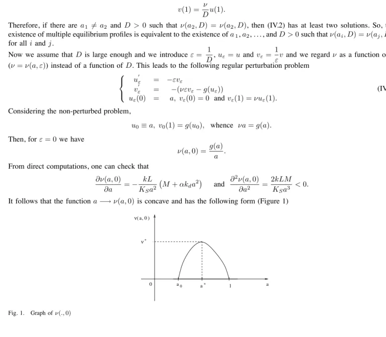
From direct computations, one can check that ∂ν(a, 0) ∂a = − kL KSa2 + M + αkda2, and ∂ 2ν(a, 0) ∂a2 = 2kLM KSa3 < 0.
It follows that the function a−→ ν(a, 0) is concave and has the following form (Figure 1)
0 a0 a* 1 a ) * ν ν( a, 0 Fig. 1. Graph of ν(., 0)
From the Theorem of dependence of the solutions of ordinary differential equations on initial conditions, lim
ε→0ν(a, ε) = ν(a, 0) in C
2[0, 1].
It follows that there exists ε∗> 0 such that for any 0≤ ε ≤ ε∗, the equation (IV.4) has
(i) at least two non trivial solutions for 0≤ ν < ν∗,
(ii) at least one non trivial solution for ν = ν∗,
A. Numerical illustration
Numerical simulations have been performed in order to illustrate the existence of multiple equilibrium profiles for the tubular biochemical reactor model. The following values of the model’s parameters are considered :
Sin= 10; Ki= 5; µ0= 0.65; kd= 0.26; D = 1.3; L = 1; k = 7; KS = 3; and ν = 0.03.
It is shown that besides the trivial equilibrium (0, 0), there exist two non trivial equilibrium profiles (¯x1, ¯x2) and (x∗1, x∗2)
represented in Figure 2 and Figure 3. The equilibrium profiles satisfy the inequalities 0 ≤ ¯x1(z) ≤ x∗1(z), for all z ∈ [0, 1]
Recall that
¯x1= Sin− ¯S
Sin ,
where ¯S is the corresponding substrate concentration at equilibrium. So, in both Figures 2 and 3, the substrate concentration
is decreasing along the reactor. In Figure 3, the biomass concentration X∗ is also decreasing along the reactor. Indeed, in
this case the substrate concentration S∗ is too small and so the death effect becomes more important than the growth for the
biomass. x10−3 x1(z) z 0.0 0.1 0.2 0.3 0.4 0.5 0.6 0.7 0.8 0.9 1.0 252.000 252.440 252.880 253.320 253.760 254.200 z x10−3 x2(z) 0.0 0.1 0.2 0.3 0.4 0.5 0.6 0.7 0.8 0.9 1.0 1.00 1.22 1.44 1.66 1.88 2.10
Fig. 2. Nontrivial equilibrium (¯x1, ¯x2)
x10−3 z x*1(z) 0.0 0.1 0.2 0.3 0.4 0.5 0.6 0.7 0.8 0.9 1.0 991.700 992.112 992.525 992.938 993.350 993.763 994.175 994.587 995.000 z x10−3 x*2(z) 0.0 0.1 0.2 0.3 0.4 0.5 0.6 0.7 0.8 0.9 1.0 2.500 2.714 2.929 3.143 3.357 3.571 3.786 4.000
Fig. 3. Nontrivial equilibrium (x∗ 1, x∗2)
V. STABILITY OF EQUILIBRIUM PROFILES
The stability of equilibrium profiles of the biochemical reactor dimensionless model (II.6)-(II.9) is analyzed here. This analysis is based on the linearized equations at the equilibrium. As in Lemma 3.8, one can see that the semigroup associated with the linearized equations is compact and by [23, Theorems 11.20 and 11.22], the stability of equilibria is determined by the eigenvalue problem. We first prove that the trivial equilibrium (0, 0) is locally asymptotically stable. Among the multiple equilibrium profiles, it is shown that the middle one (¯x1, ¯x2) is unstable whereas the third equilibrium profile (x∗1, x∗2) is locally
asymptotically stable.
Let us consider an equilibrium solution (¯x1, ¯x2) of (II.6)-(II.9). Recall that
¯x2=(1 − ¯x1 )(M + αkd¯x1) kdKS and ˜µ(¯x1, ¯x2 ) = µ0 β (1 − ¯x1) KS¯x2+ (1 − ¯x1) + α(1 − ¯x1)2, for all z∈ [0, 1]. (V.1)
Let us introduce for i = 1, 2,
ϕi(z) = β µ0 ∂ ∂ui (˜µ(u1, u2)u2) |(u1,u2)=(¯x1(z),¯x2(z)).
It follows from direct computations, by using (V.1), that ϕ1(z) = 1 µ2 0KS (M + αkd¯x1(z))(kd− µ0+ 2αkd(1 − ¯x1(z))), for all z ∈ [0, 1] and ϕ2(z) = kd µ2 0 (kd+ αkd(1 − ¯x1(z))), for all z ∈ [0, 1].
The linearized system of (II.6)-(II.9) at (¯x1, ¯x2) is given by
∂x1 ∂t = 1 Pe ∂2x 1 ∂z2 − ∂x1 ∂z + kµ0 β ϕ1(z)x1+ kµ0 β ϕ2(z)x2, ∂x2 ∂t = −γx2+ µ0 β ϕ1(z)x1+ µ0 β ϕ2(z)x2, ∂x1 ∂z (t, 0) = Pex1(t, 0) and ∂x1 ∂z (t, 1) = 0. (V.2)
The stability of the equilibria is determined by the eigenvalue problem 1 Pe x!!1 − x ! 1+ kµ0 β ϕ1(z)x1+ kµ0 β ϕ2(z)x2 = λx1, −γx2+ µ0 β ϕ1(z)x1+ µ0 β ϕ2(z)x2 = λx2, 1 Pex ! 1(0) = x1(0) and x ! 1(1) = 0. (V.3)
A. Stability of the trivial equilibrium (0, 0)
For the trivial equilibrium, the functions ϕ1 and ϕ2 are constant and given by
˜ ϕ1= ϕ1(z) = M (αkd− M) µ2 0KS < 0, for all z∈ [0, 1], ˜ ϕ2= ϕ2(z) = k2 d(1 + α) µ2 0 > 0, for all z∈ [0, 1]. The parameters are assumed to satisfy the following condition.
A1 : kd(1 + α) < µ20 ' L ν∗ (2 . Hence, the following result holds.
Proposition 5.1: Assume that A1 holds. Then the trivial equilibrium (0, 0) is locally asymptotically stable. Proof : First of all, observe that if
λ≤ −γ +µ0
β ϕ˜2
then under assumption A1, λ < 0 and therefore the equilibrium profile (0, 0) is locally asymptotically stable. Now assume that
Then from the second equation of (V.3), x2 can be expressed as follows x2= µ0 β ϕ˜1 λ + γ−µ0 β ϕ˜2 x1= ˜bx1. We set also a = kµ0 β ϕ˜1< 0 and b = kµ0 β ˜b < 0. The problem (V.3) is reduced to the following one :
1 Pe x!!1− x ! 1+ (a + b − λ)x1 = 0, 1 Pe x!1(0) = x1(0) and x ! 1(1) = 0.
Let us introduce the following variables
u(z) := e−Pe2zx1(z), v(z) := u((z), for all z∈ [0, 1].
The equations above are equivalent to the following ones u( = v, v( = P e 'P e 4 + λ − a − b ( u, v(0) = Pe 2 u(0) and v(1) =− Pe 2 u(1). (V.5)
A necessary condition for equations (V.5) to have a solution is that Pe
4 + λ − a − b < 0. It turns out that λ must satisfy
λ <−Pe
4 + a + b < 0.
It follows that the trivial equilibrium profile (0, 0) is locally asymptotically stable. !
Now we shall consider that there exist two nontrivial equilibrium profiles (¯x1, ¯x2) and (x∗1, x∗2) as determined by Proposition
4.1. Note that the equilibrium profiles satisfy
0 ≤ ¯x1(z) ≤ x∗1(z), ∀ z ∈ [0, 1].
We shall first deal with the the stability of the nontrivial equilibrium profile (x∗1, x∗2). B. Stability of the nontrivial equilibrium (x∗
1, x∗2)
Observe that the function ϕ2 is positive and decreasing in [0, 1]. Also,
ϕ1(z) > 0, for all z ∈ [0, 1] such that x∗1(z) ∈
-−M αkd , 1 2 − M 2αkd -, ϕ1(z) < 0, for all z ∈ [0, 1] such that x∗1(z) ∈
-1 2 − M 2αkd , 1 . and if x∗ 1(z) ∈ [14− 3M
4αkd, 1] for all z∈ [0, 1], then ϕ1 is decreasing.
Let us consider the eigenvalues problem (V.3). Observe that if there exists z0∈ [0, 1] such that
λ + γ−µβ0ϕ2(z0) ≤ 0
then, by using assumption A1, one has λ < 0. Also, if λ + γ≤ 0 then λ < 0. Therefore, we shall assume that
λ + γ > 0 and λ + γ−µ0
It follows from equation (V.3) that x2= µ0 β ϕ1(z) λ + γ−µ0 β ϕ2(z) x1 (V.7) and 1 Pe x!!1 − x ! 1+ µ0k β ϕ1(z)x1+ µ0k β ϕ2(z)x2 = λx1, 1 Pe x!1(0) = x1(0), x ! 1(1) = 0.
One can deduce from the Krein-Rutman theory that x1 never changes sign. Without loss of generality, we can assume that x1
is positive and as (x1, x2) is an eigenvector then x1 is strictly positive. Let us introduce the following variables
u(z) := e−Pe2 zx1(z) and v(z) := u!(z), for all z∈ [0, 1].
Then (considering also (V.7)) u! = v, v! = Pe & Pe 4 + λ − µ0k β λ + γ λ + γ−µ0 βϕ2(z) ϕ1(z) ) u, v(0) = P2eu(0), v(1) =−P2eu(1). (V.8)
First : Observe that if x∗
1 is in the interval [12− M
2αkd, 1] then ϕ1(z) is negative for all z ∈ [0, 1]. Hence, reminding (V.6), a
necessary condition for (V.8) to have a solution is λ < 0.
Let us consider now the opposite case and let us make the following assumptions.
A2 : 14 −4αk3M d ≤ / −M αkd and 1 4 − 3M 4αkd ≤ x ∗ 1(z), for all z ∈ [0, 1].
Observe that if λ is a very large positive number then v!(z) is always strictly positive and (V.8) cannot have a solution.
Therefore, there exists λmax such that λ + γ ≤ λmax+ γ. Also, from (V.6), there exists a strictly positive number C0 such
that λ + γ−µ0
βϕ2(z) ≥ C0 for all z∈ [0, 1].
Second : Observe that if x∗
1 is such that ϕ1(z) is positive for all z ∈ [0, 1] i.e. x∗1(z) ∈ [14− 3M 4αd, 1 2− M 2αd] for all z ∈ [0, 1],
then the function
z−→ −µ0k β & λ + γ λ + γ−µ0 βϕ2(z) ) ϕ1(z)
is increasing in [0, 1]. Hence, a necessary condition for (V.8) to have a solution is Pe 4 + λ − µ0k β & ( λ + γ λ + γ−µ0 βϕ2(0) ) ϕ1(0) < 0.
There exists a positive number ¯A (depending on x∗
1) such that Pe 4 + λ − µ0k β & ( λ + γ λ + γ−µ0 βϕ2(0) ) ϕ1(0) − ¯A < 0.
We make the following assumptions
A3 : A¯≥ maxi=1,2 * a0 % 1 0 |ϕ ! 1(z)|dz + ai % 1 0 |ϕ 1(z)ϕ ! 2(z)|dz 0 , A4 : a0 % 1 0 |ϕ 1(z)|dz < 1, where a0= µ0k β λmax+ γ C0 , a1 =µ20k β2 λmax+ γ C2 0 , a2= µ2 0k β2 1 λmax+ γ.
Under assumption A3, the solution (u, v) of (V.8) satisfies 1 1 1 1v(z)u(z) 1 1 1 1 ≤ P2e, ∀ z ∈ [0, 1]. Introducing θ := v u leads to |θ(z)| ≤ P2e, ∀ z ∈ [0, 1] (V.9)
and (by using (V.7))
θ! = Pe & Pe 4 + λ − µ0k β λ + γ λ + γ−µ0 β ϕ2(z) ϕ1(z) ) − θ2, θ(0) = Pe 2 , θ(1) =− Pe 2 , (V.10)
Integrating this equation leads to
−Pe= P2 e 4 − % 1 0 θ2(z)dz + Pe & λ−µ0k β % 1 0 ϕ1(z) & λ + γ λ + γ−µ0 βϕ2(z) ) dz ) . By using (V.9), one has
Peλ≤ Pe & −1 +µβ0k % 1 0 ϕ1(z) & λ + γ λ + γ−µ0 βϕ2(z) ) dz ) . Then, by assumptions A3-A4, it follows that λ < 0.
Third : Let us consider now the case when there exists z0∈]0, 1[ such that
x∗1(z) ∈ - 1 4 − 3M 4αkd , 1 2 − M 2αkd .
for all z∈ [0, z0] and x∗1(z) ≥
1 2 −
M 2αkd
, for all z∈ [z0, 1].
Two situations are possible. If v!(0) < 0 then by using assumptions A3-A4 and the arguments given in the previous case, one
has λ < 0. On the opposite case, we have v!(z) ≥ 0 for all z ∈ [0, z0] and as in the first part (of the subsection) a necessary
condition for (V.8) to have a solution is λ < 0 since Pe 4 − µ0k β λ + γ λ + γ−µ0 βϕ2(z) ϕ1(z) > 0, for all z ∈ [z0, 1].
In view of the arguments above, the following statement holds :
Proposition 5.2: Assume that A1-A4 hold. Then the nontrivial equilibrium profile (x∗1, x∗2) is locally asymptotically stable. C. Instability of the nontrivial equilibrium profile (¯x1, ¯x2)
Let us consider the functionals
Q1(x1, x2) = % 1 0 ' −P1 e|x ! 1|2+ µ0k β ϕ1(z)x 2 1+ µ0k β ϕ2(z)x1x2 ( dz−1 2 + x21(0) + x21(1) , %x1%22 , Q2(x1, x2) = % 1 0 ' −γ|x2|2+ µ0 β ϕ2(z)x 2 2+ µ0 β ϕ1(z)x1x2 ( dz %x2%22 ,
where%xi%2 is the L2-norm of xi on [0, 1]. Observe that if (x1, x2) is an eigenvector of (V.3) then necessarily Q1(x1, x2) =
Q2(x1, x2) and is the corresponding eigenvalue. As in the idea of [23, Theorem 11.6], one can see that the principal eigenvalue
λ1is an increasing function of Pe. Then λ1(Pe) ≥ λ1(0). Therefore, one has to consider the case Pe= 0. Let us first introduce
ε = Pe, uε(z) := x1(z), vε(z) := 1
εx
!
One can deduce from (V.3) that u!ε = εvε, vε! = ' εvε− µ0k β ϕ1(z)uε− µ0k β ϕ2(z)wε+ λuε ( , vε(0) = uε(0), vε(1) = 0.
For ε = 0, the equilibria as well as the eigenfunctions are scalar and by integrating the equation above, one has : −uε(0) = −µ0k β ϕ1(0)uε(0) − µ0k β ϕ2(0)wε(0) + λuε(0). Therefore, λ(0)uε(0) = ( µ0k β ϕ1(0) − 1)uε(0) + µ0k β ϕ2(0)x2(0). It is easy to see that ¯x1 is a zero of the function
a∈ -−αkM d , 1 . → k ˜µ(a, ¯ax2)¯x2 − 1
and that the derivative of this function at ¯x1 is strictly positive. Hence, µβ0kϕ1(0) − 1 > 0. On the other hand, one can see
from the expression of ϕ2(z) that it is always positive. It follows that the eigenvalue λ1(0) is strictly positive and this holds
for all Pe> 0.
In view of the arguments above, the following statement holds
Proposition 5.3: The non trivial equilibrium profile (¯x1, ¯x2) is unstable.
VI. CONCLUDING REMARKS
This paper was devoted to the dynamical analysis of a tubular biochemical reactor nonlinear model. The dynamics of these reactors are described by distributed parameter systems. More specifically, a system of nonlinear partial differential equations was studied. The existence of the state trajectories and the invariance of the set of physically feasible state values under the dynamics of the reactor as well as the convergence of the state trajectories to equilibrium profiles of the dynamical model were proved. The multiple existence and stability of equilibrium profiles were analyzed under physically meaningfull conditions. It was proved that, depending on the axial dispersion parameter, the dynamical model can have two stable and one unstable equilibrium profiles. In this study, it is shown that, for large values of axial dispersion parameter, the tubular biochemical behaves like a stirred tank reactor. And, as for completely mixed systems, the system studied here can have an unstable equilibrium which can coincide with an interesting operating point in practical viewpoint. So, as perspectives for further researches, we shall be interested in the control of this system which is nonlinear and infinite dimensional.
ACKNOWLEDGMENTS:
This paper presents research results of the Belgian Programme on Inter-University Poles of Attraction initiated by the Belgian State, Prime Minister’s office for Science, Technology and Culture. The scientific responsability rests with its authors.
REFERENCES
[1] J. F. Andrews ; A mathematical model for the continuous culture of microorganisms utilizing inhibitory substrates, Biotechnology and Bioengineering, Vol. 10, pp. 707-723, 1968.
[2] G. Bastin and D. Dochain ; One-line Estimation and Adaptive Control of Bioreactors, Elsevier, Amsterdam, 1990.
[3] O. Bernard, Z. Hadj-Sadok, D. Dochain, A. Genovesi and J. -P. Steyer ; Dynamical model development and parameter identification for an anaerobic wastewater treatment process, Biotech. Bioeng., Vol. 75, pp. 424-438, 2001.
[4] A. Bertucco, P. Volpe, H. E. Klei, T. F. Anderson and D. Sundston ; The stability of activated sludge reactors with substrate inhibition kinetics and solid recycle, Water Research, Vol. 24, No. 2, pp. 169-176, 1990.
[5] P. D. Christofides and P. Daoutidis ; Nonlinear feedback control of parabolic PDE systems, In Nonlinear Model Based Process Control ; R. Berber and C. Kravaris (eds), Kluwer, Dordrecht, 1998.
[6] D. Dochain ; Contribution to the Analysis and Control of Distributed Parameter Systems with Application to (bio)chemical Processes and Robotics, Thse
de Doctorat d’Etat, CESAME, Universit Catholique de Louvain, Belgique, 1994.
[7] A. K. Dram´e ; A semilinear parabolic boundary-values problem in bioreactors theory, Electronic Journal of Differential Equations, Vol. 2004(2004), No 129, pp. 1-13.
[8] A. K. Dram´e, J. Harmand, A. Rapaport and C. Lobry ; Multiple steady state profiles in interconnected biological systems, Mathematical and Computer
Modelling of Dynamical Systems, Vol. 12, No. 5, October 2006, 379-393.
[9] A. Friedman ; Partial differential equations of parabolic type, Prentice-Hall, Englewood Cliffs, 1964.
[11] M. Laabissi, M. E. Achhab, J. J. Winkin and D. Dochain ; Trajectory Analysis of nonisothermal tubular reactor nonlinear models, Systems and Control
letters, 42, 2001, pp. 169-184.
[12] M. Laabissi, M. E. Achhab, J-J. Winkin and D. Dochain ; Multiple equilibrium profile for nonisothermal tubular reactor nonlinear model, Dynamics of
Continuous, Discrete and Impulsive Systems, Vol. 11, 2004, 339-352.
[13] M. Laabissi, J. J. Winkin, D. Dochain and M. E. Achhab ; Dynamical Analysis of a Tubular Biochemical Reactor Infinite-Dimensional Nonlinear Model,
Proc. 44th IEEE CDC-ECC, 2005, pp. 5965-5970.
[14] H. Matano ; Convergence of solutions of one-dimensional semilinear parabolic equations, J. Math. Kyoto Univ. 18-2 (1978), 221-227. [15] H. Matano ; Asymptotic behavior and stability of solutions of semilinear diffusion equations, Publ. RIMS, Kyoto Univ., 15, 401-454 (1979). [16] R. H. Martin ; Nonlinear Operators and Differential Equations in Banach Spaces, John Wiley and Sons, New York, 1976.
[17] R. Nagel (ed.) ; One-parameter Semigroups of Positive Operators, Lecture notes in mathematics, 1184, Springer Verlag, New York, 1986. [18] A. Pazy ; Semigroups of Linear Operators and Applications to Partial Differential Equations, Springer Verlag, Berlin, 1983.
[19] U. Pawlowsky, J. A. Howell and C. T. Hi ; Mixed culture bioxidation of phenol, III. Existence of multiple steady state in continuous cultures with wall growth, Biotechnology and Bioengineering, Vol. 15, pp. 905-916, 1976.
[20] M. H. Protter and H. F. Weinberger ; Maximum principles in differential equations, Prentice-Hall, Englewood Cliffs, 1967.
[21] O. Schoefs, D. Dochain, H. Fibrianto and J. -P. Steyer ; Modelling and identification of a partial differential equation model for an anaerobic wastewater treatment process, Proc. 10th World Congress on Anaerobic Digestion (AD01-2004), Montr´eal, Canada.
[22] H. L. Smith ; Monotone dynamical systems : An introduction to the theory of competitive and cooperative systems, Math. Surveys Monogr. 41, AMS, Providence, RI, 1995.
[23] J. Smoller ; Shock waves and reaction-diffusion equations, Springer-Verlag, New-York, 1983.