Characterisation of the electric drive of EV: on-road versus off-road method
27
0
0
Texte intégral
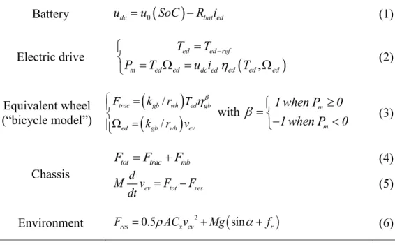
Figure
![Table 2. Electric vehicle parameters 146 parameter value gearbox ratio k gb 5.84 gearbox efficiency gb 0.98 wheels radius r wh [m] 0.2865 curb mass [kg] 562 A·C x [m 2 ] 0.7 f r 0.02](https://thumb-eu.123doks.com/thumbv2/123doknet/14606101.731762/10.893.315.580.167.385/table-electric-vehicle-parameters-parameter-gearbox-gearbox-efficiency.webp)
+7
Documents relatifs
