FINAL REPORT
ESTIMATES OF ICE LOADS ON THE MOLIKPAQ at
AMAULIGAK I-65 BASED ON GEOTECHNICAL
ANALYSES AND RESPONSES
Kevin Hewitt, P.Eng. K.J. Hewitt & Associates Ltd.
Calgary January 15th, 2010
TABLE OF CONTENTS
Page
EXECUTIVE SUMMARY 3
INTRODUCTION 3
GEOTECHNICAL DESIGN of the MOLIKPAQ 5
• Importance of Core Sand Properties
METHODS OF ASSESSING IN SITU SAND STATE 8
• Relative Density
• Cone Penetration Test (CPT) • Pressuremeter Tests
• Placement Technique
INSITU STATE of the CORE SAND AT AMAULIGAK I-65, 1986 12
ANALYTICAL MODELS 16
• General
• Geotechnical Models o EBA model o GCRI models o Hicks & Smith, 1988 o Altaee & Fellenius, 1994 o Jeyatharan, 1991 • Sandwell Structural model
PERFORMANCE PREDICTIONS 25
• Geotechnical Models o EBA model o GCRI models o Hicks & Smith, 1988 o Altaee & Fellenius, 1994 o Jeyatharan, 1991
• Summary of Geotechnical Models • Best Estimate Geotechnical Model • Sandwell Structural model
MEASURED DISPLACEMENTS 32
• General
• Slope Indicators • Extensometers
ICE LOAD ESTIMATES 42 • Using Best Estimate Geotechnical Model
• Using Sandwell Structural Model • Using Other Means
o Molikpaq May 12th Event
o SSDC at Kogyuk, 1983 o Hans Island, 1983
SUMMARY 48
CONCLUSIONS 51
REFERENCES 52
COMMENTS ON KLOHN CRIPPEN BERGER REPORT 55
EXECUTIVE SUMMARY
This report documents a review of the response of the Molikpaq to ice loading at the Amauligak I-65 site in 1986, primarily from a geotechnical perspective. This included a review of:
• The initial design which emphasized the importance of the core sand properties.
• The as-placed (in situ) state of the core sand at Amauligak.
• Performance predictions based on various models, both geotechnical and structural.
• Measured displacements.
As a result, ice load estimates were made for several events. The largest estimated load was during the event on the morning of April 12th, 1986. It is the author’s opinion that since the global displacements were relatively small and that the sand core was in a loose state that this load was about 200 MN. However because of the inherent uncertainties in the evaluation of the properties of the composite unit combined with the uncertainties in determining displacements, it is believed that the actual load could differ from this estimate. Therefore it is the author’s opinion that the load could have been as high as 250 MN or as low as 150MN.
These estimated values for the April 12th morning event are consistent with loads determined for other ice interactions, including those at Hans Island, which are based on mass decelerations. However they are in the order of 50% or less than loads previously estimated by others which either directly or indirectly rely on Medof panel data.
INTRODUCTION
In order to conduct year-round drilling in the Beaufort Sea, which is ice covered for the majority of the year, a platform must resist significant ice forces. In the 1970’s and early 1980’s the understanding of ice-structure interaction was quite limited which led to very conservative design global ice loads. This situation led to the construction of massive ‘structures’ in the form of artificial islands composed of dredged sand fill. In deeper waters such an approach was not viable as the islands could only be constructed with relatively flat side slopes which resulted in very large fill volumes (volumes increase exponentially with water depth). This led to caisson systems capable of penetrating the water line and greatly reducing sand volumes.
The Molikpaq, consisting of a steel annular box with a simply supported steel deck supporting the drilling rig and associated modules, was one such caisson system. The Molikpaq has since been converted to a production platform and is in use offshore Sakhalin Island. The original Molikpaq caisson was designed to
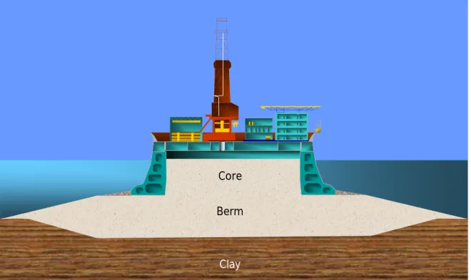
transfer ice loads to its base and a central sand core and could be deballasted for relocation to a subsequent well site. The caisson was a chamfered square in plan with outside base dimensions of 111m. The inner core section was 72m square and was designed to be filled with sand to a height of approximately 21m. With respect to the Tarsiut P-45 (1984/85), Amauligak I-65 (1985/86) and Amauligak F-24 (1987/88) sites the steel structure and its sand core rested on a sand berm which in turn rested on a prepared area on the seafloor (see figure 1). The main difference between these three deployments was that the core was not densified at the first two sites, including the subject Amauligak I-65 site, but was subsequently densified using explosives at the Amauligak F-24 site.
Core Berm
Clay
Figure 1 Schematic of Molikpaq as deployed
During the winter of 1986, while at the I-65 location in a water depth of 31 metres, the Molikpaq was subjected to a number of impacts by multi-year ice. The purpose of this report is to provide estimates of the ice loads associated with these impacts based on geotechnical analyses and responses.
In summary, the report shows, that because the sand core was in a loose state and because displacements were relatively small, that the ice loads estimated from geotechnical analyses and responses were a lot less than previously documented. The report’s conclusion is that the ice loads experienced by the Molikpaq at I-65 were in the order of 50% or less than loads estimated by other means which either directly or indirectly rely on Medof panel data. Conversely
the estimated loads are consistent with loads that do not rely on Medof panel data such as those based on the structural response of the Molikpaq and those based on floe decelerations including Hans Island data.
GEOTECHNICAL DESIGN of the MOLIKPAQ
According to Jefferies et al (1985), ‘The structure has two distinct load paths for
lateral ice loading. Some of the ice load is transferred into the berm by caisson base friction; the load transferred in this manner typically varies between 10 and 25%. The balance of the load, in excess of 75%, is transferred into the sand core….(As such) the Molikpaq stability is most appropriately assessed by methods developed for horizontally loaded earth structures in contrast to bearing capacity methods usually used with gravity based structures.’ (NOTE: It is
explained later in this report that, for low loads, the majority of the load is transferred into the base. It is not until the ice load reaches close to the ultimate capacity of the composite platform that the majority of the load, in the order of 75%, is transferred to the core.)
An appreciation for the relative contributions of the caisson and the core in resisting horizontal loading, at the limit, can be obtained by comparing their vertical loadings. ‘The dead load of the Molikpaq structure when ballasted onto
the berm is approximately 320 MN which corresponds to the “lightship” condition. However a much greater dead load occurs because of the sandfill in the core which has a submerged weight of about 1,000 MN’. (Jefferies et al., 1985)
(NOTE: Under operating conditions the net structure weight would be higher.) Importance of Core Sand Properties
Because the majority of the ultimate resistance to horizontal loading is derived from the sand core, the in situ properties of this core sand need to be well understood in order to undertake predictions regarding the performance of the structure under static or dynamic ice loading. However these properties have less influence on the load displacement curve of the composite unit at lower loads when the majority of the load is transferred into the base. It was clearly recognized at the design stage that the properties of the sand in the core of the Molikpaq were critical to lateral stability. McCreath et al (1982) state that ‘The
performance of the composite system under load will be primarily a function of the geotechnical parameters of the foundation materials and of the sand fill which is utilized in the core and berm.’
They go on to state that, with respect to the sand core, ‘while the assumption of
drained conditions under static loading is reasonable, the analyses do show that if any positive pore pressure is generated during shearing, due to contractive action of the sand and slow drainage response, the computed factor of safety declines rapidly. For this reason, it was concluded that the sand must be placed at a density which assured dilative action during shear.’
It was also recognized that ‘Due to the wind driven nature of the ice,
monotonically pulsating ice loads may be applied to the structure… these loads may apply several hundreds of cycles of load to the structure, giving rise to concern regarding potential liquefaction or cyclic mobility of the sand core’.
Based on laboratory steady state testing, McCreath et al. concluded that ‘true’ liquefaction would be possible for relative densities of the sand core of less than 25 percent. However they note that even for more dense sand states there is
‘…the potential problem of generating large cyclic mobility strains due to many cycles of monotonically repetitive ice loading. During repetitive loading, pore pressures will be generated within the sand, and the rate at which such pore pressures dissipate is not easy to quantify.’
Bruce and Harrington (1982) stated that ‘For overall stability, dense sand is
required in the core of the annulus and in the berm…..Provisions for the addition of densification equipment have been incorporated in the design.’ McCreath et al
(1982) make similar statements: ‘Thus, it may be concluded that densification of
the core fill sand to relative densities of about 70% is a sufficient condition to avoid serious cyclic mobility problems.’ ‘Available methods for achieving the required density in the sand fill have been carefully reviewed… . However, such densification would require some advance upon the state-of-the-art in vibro-compaction. The major implications of a requirement for densification would be both in terms of capital cost and in terms of schedule delay.’
Subsequent to the conclusions reached above, the engineers responsible for the first Molikpaq deployment in 1984 at Tarsiut P-45 concluded that the use of relative density to characterize sand state was inappropriate. They therefore developed a new concept they termed the ‘state parameter’ (the sand state relative to the steady state) which they believed was a more appropriate parameter to use in design (Been and Jefferies, 1985).
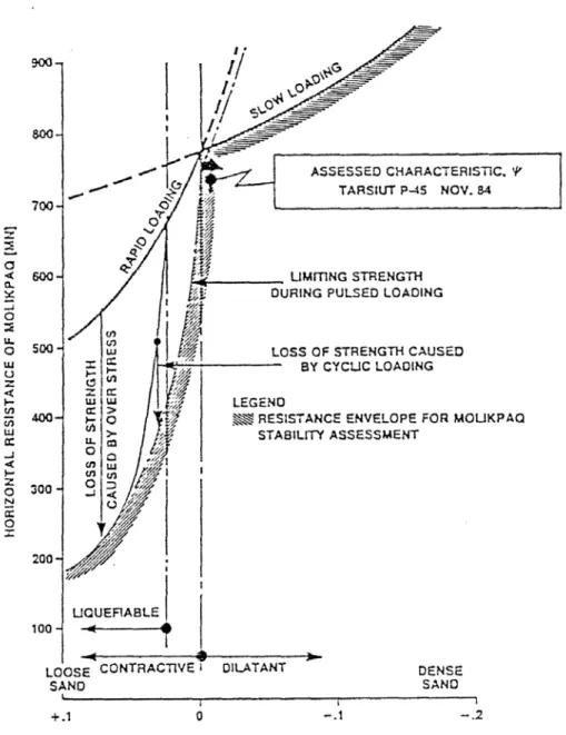
It was concluded that a state parameter of less than zero was required for adequate performance. Figure 2 is reproduced from the paper by Jefferies et al (1985). It shows the predicted horizontal resistance to ice load versus the core sand state parameter. Jefferies et al point out that ‘significant performance
shortfalls should be expected if the characteristic state of the sand is looser than zero (i.e.; positive state). Specifically this figure shows that under pulsed ice
loading the horizontal resistance to ice load reduces rapidly for state parameters greater than zero.
Adoption of the state parameter approach had the advantage (at the time) that a recently performed interpretation of laboratory test data apparently had shown that the state parameter could be directly correlated to CPT tip resistance. This correlation simplified core density verification. However this correlation was subsequently shown to be in error by a substantial amount (Sladen, 1989). This topic is discussed further on page 15.
Figure 2: Design Predictions of Molikpaq Horizontal Load Capacity as a Function of Core Sand Density (from Jefferies et al, 1985)
As discussed above, the insitu state of the core sand is critical to evaluating the core sand’s behaviour and hence the performance of the Molikpaq under ice loading. However the behaviour of sand is sensitive to small differences in void ratio (the ratio of the volume of voids to the volume of solids). Therefore this void ratio must be quantified in order to predict performance.
METHODS OF ASSESSING IN SITU SAND STATE (RELATIVE DENSITY) Relative Density
Attempts to define the possible range of void ratios have led to the concept of a maximum (loosest) and a minimum (densest) void ratio. If the method of achieving these two void ratios is standardized (i.e. ASTM D2049-69), then the actual void ratio can be defined in terms of relative density (i.e. density relative to the loosest and densest states). The range of relative densities from 0% to 100% corresponds to the range of sand densities defined in geotechnical terms from very loose, loose, medium, dense through to very dense.
The following table 1 has been prepared for future reference. It also shows a very approximate correlation between relative density and ‘state parameter’, well realizing that the two terms cannot be directly related. However it is felt that this comparison will assist the reader when state parameter values are quoted.
DESCRIPTIVE TERM RELATIVE DENSITY RANGE (%) ‘STATE PARAMETER’ (APPROXIMATE) Very loose 0 to 15 +0.20 to +0.14 Loose 15 to 35 +0.14 to +0.06 Medium dense 35 to 65 +0.06 to -0.06 Dense 65 to 85 -0.06 to -0.14 Very dense 85 to 100 -0.14 to -0.20
Table 1: Approximate correlation between relative density and ‘state parameter’ However because the numerical differences in void ratio between the two states (loosest and densest states) are not that large, errors in the determination of the insitu void ratio, and the maximum and minimum ratios, can be compounded when assessing relative density. Errors are also inherent in determining the insitu void ratio as it is difficult to recover a sample of sand with any certainty that its void ratio has not changed during the sampling process.
This has led to many attempts to measure in situ density indirectly by correlation to the results of insitu tests. Such tests have included the Standard Penetration Test (SPT), the self boring pressuremeter and the Cone Penetration Test (CPT). Another indirect method to determine insitu density is based on the placement technique. The SPT, although it gives a qualitative indication of density, has proven to be less than reliable for quantitative assessments. It was therefore not used as a testing method for the Molikpaq.
Cone Penetration Test (CPT)
The CPT is favoured by many engineers because it is widely available and standardized, it does not rely on minimizing disturbance during insertion, it
provides a continuous profile of the measured parameters and there is a large body of literature concerning its interpretation.
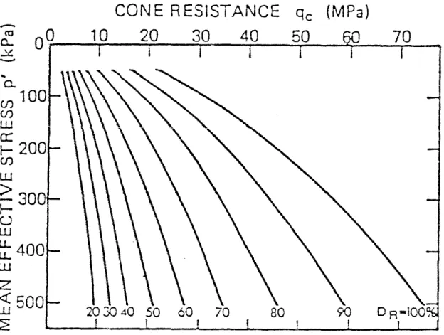
Various researchers have used large scale chamber tests to determine relationships between sand density, or void ratio, mean effective stress level and CPT tip resistance. For a given sand there is a unique relationship between these parameters. The most extensive and complete data sets for a clean sand are provided by Baldi et al., 1986. The correlations presented in the Baldi et al paper are shown as figure 3. Although these correlations may not be directly applicable to the Erksak sand used in the Molikpaq core at Amauligak, they have proven useful in evaluating densities of hydraulically placed Beaufort sands in general (Sladen & Hewitt, 1989).
Figure 3: The relationship Between Cone Resistance and Relative Density (From Baldi et al, 1986)
Pressuremeter Tests
While there are no general correlations to relate the results of self-bored pressuremeter tests directly to either relative density or state parameter, there has been much work aimed at evaluating the degree of dilation, or dilation angle.
Interpretations of the pressuremeter are generally based on theoretical considerations with only limited laboratory data.
While the general validity of these relationships to all sands is not known they do provide a useful, relative index of in situ state. For example, the higher the inferred dilation angle the denser the sand is likely to be (or the lower the state parameter is likely to be).
Placement Technique
It is of interest to compare the placement of hydraulic fills beneath water, which involves settling from a slurry, with the basic test methods used to establish maximum and minimum void ratios for sands (i.e. gentle pluviation versus compaction on a vibrating table). Since there is a large difference in energy input in the basic test methods, it would seem implausible that any form of hydraulic placement could result in a relative density significantly closer to the maximum than the minimum. In other words it would be unreasonable to expect an uncompacted hydraulically placed sand to have a dense or very dense state of packing.
Indeed it is intuitive to expect that material pumped as a slurry from a pipeline and allowed to settle gently through water would have a relative density close to the minimum (very loose). It would be reasonable however to expect that if a free-draining sand were placed using a technique that imparted some compactive effort (i.e. depositing as a lump mass), a denser condition might be achieved (say loose to medium dense). Likewise it would not be unreasonable to expect that a certain placement technique would result in a certain fairly narrow range of values of relative density.
Two basic methods of placement of hydraulic sand fills have been used in the Canadian Beaufort Sea; (1) Hopper placement or bottom dumping, and (2) Pipeline placement. The first involves the release of large quantities of sand from openings in the base of a barge or dredge without pumping. Sand, so deposited, drops to the seabed as a ‘slug’ or dense flume and the kinetic energy is dissipated when the material impacts the seabed (or the previously deposited sand). The energy of impact densifies the sand. This method can only be used for subaqueous fills in water depths of more than about 8 to 9 metres. For the pipeline placement method, sand suspended in water is pumped through a pipe and discharged on the surface being filled. The volume of water involved is of necessity much greater than the volume of sand particles. This method can be used for both underwater and above water depositions.
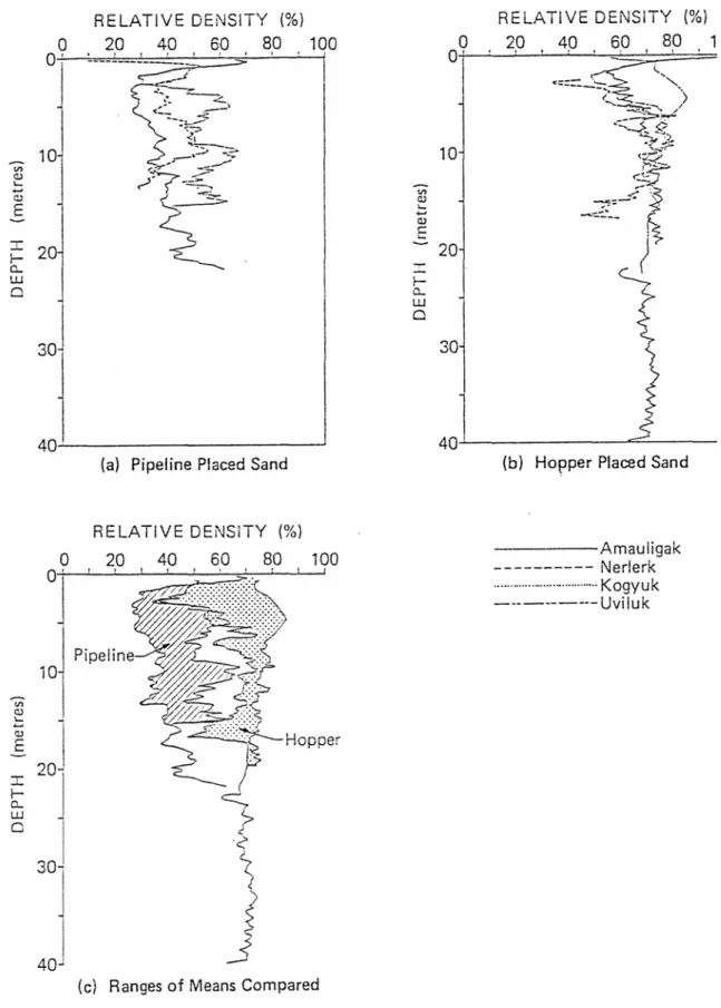
Data obtained from several artificial islands constructed in the Canadian Beaufort Sea have provided evidence that material placed by bottom dumping is significantly denser than pipeline placed material, all other factors being equal (Sladen & Hewitt, 1989). This is consistent with expectations. The data show
Figure 4: Comparative Profiles of Mean Relative Density for Hopper and Pipeline Placed Sands (Sladen & Hewitt, 1989)
that, in terms of relative density, hopper placed sand is typically 30 to 40% denser than pipeline placed material (see figure 4).
INSITU STATE of the CORE SAND AT AMAULIGAK I-65, 1986
Core filling was achieved by discharging the contents of a trailing suction hopper dredge into a floating pipeline; this pipeline being connected to the built-in piping of the Molikpaq. The built-in piping fed the slurry to discharge from a single, near central 800mm diameter spigot (i.e. equivalent to pipeline placement). The discharge elevation was approximately at sea level. This method of placement would favour the sand being placed in a loose state. In fact it would be difficult to devise a method to ensure a looser state. The procedure for obtaining the minimum density in the laboratory actually models this placement method.
At both the first deployment of the Molikpaq at Tarsiut P-45 (1984/85) and the second deployment at Amauligak I-65 (1985/86) no attempt was made to densify the core. However as a result of the poor performance at Amauligak I-65 the core was densified using explosives at the third deployment in 1987/88 at Amauligak F-24.
According to Jefferies et al, 1985, ‘The original Molikpaq concept envisaged the
use of mechanically densified fine sand. However Gulf Canada Resources Inc. (GCRI) decided not to use densification because of both cost and time considerations.’ Although these statements were made with respect to the first
Molikpaq deployment at Tarsiut P-45, the sand for the core filling and the method of placement was exactly the same as that used at the Amauligak I-65 site.
In defense of GCRI, the decision not to use densification was also obviously based on a technical evaluation. As stated earlier, GCRI had developed a correlation between the state parameter and CPT tip resistance which could be used as a direct means of verifying the adequacy of the core. Unfortunately this correlation was subsequently shown to be in error (Sladen, 1989).
Further insight to GCRI’s evaluation at the time can be gleaned from a discussion reported in the Proceedings of the Institution of Civil Engineers which includes the following comments:
‘An initial inspection of the soil material indicated that liquefaction might be a problem and that costly densification might be required. However, both semi-empirical design procedures based on laboratory testing (Casagrande’s approach) and the results of model centrifuge tests indicated that there was no problem with liquefaction under design loading conditions. As a result no densification was required, resulting in a very large saving in cost’. (Schofield and Potts, 1984).
However it is not known what sand state was used for these predictions and whether there was an appreciation at that time of the actual density achieved, based on conventional interpretations. It is also not known what drawdown in the Molikpaq core was assumed. It can be noted that at the design stage a drawdown of about 10m was expected (Bruce and Harrington, 1982) which is significantly more than was achieved at Amauligak (indications are that a drawdown of only 1.5m was achieved).
Another factor that appeared to be missing from GCRI’s technical evaluation was an issue raised in the initial Molikpaq design by McCreath et al (1982). They made the following statement:
‘The fact that the Mackenzie Delta sands may be relatively resistant to liquefaction is certainly encouraging, but does not remove the potential problem of generating large cyclic mobility strains due to the many cycles of monotonically repetitive ice loading’.
To investigate this potential problem the sand was tested under repetitive loading. One test was run on a loose sand (40% relative density) and the other on a dense sand (80% relative density). The findings were reported by McCreath et al (1982) as follows:
‘The results indicate that even after 20,000 cycles of such loading, axial strains in dense sand were less than 2%, whereas for loose sand an axial strain of more than 10% was reached in just 5 cycles. Although the sand may not have undergone true liquefaction, this point is somewhat academic, as the very large strains mobilized during undrained response of the loose sand to repetitive loading would cause a functional failure of the system’.
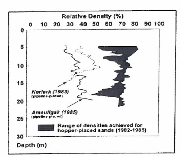
A series of CPT profiles were obtained after filling was complete. Using the Baldi et al relationship, the mean relative density of the core sand at Amauligak I-65 is shown in figure 5.
Also plotted on this figure is the density profile for the Nerlerk berm (also pipeline placed sand) which suffered flow sliding, and a range of profiles for hopper placed Beaufort Sea sands. It can be seen that (based on the Baldi et al correlation) the Amauligak I-65 core sand was loose (sand density between 30 and 40%). It is more important to note that this inferred relative density profile for the Amauligak core is the lowest of all published Beaufort Sea fills (Sladen & Hewitt, 1989).
According to Jefferies et al, 1985, The Molikpaq was intended to have a core….
with a state parameter of -0.1. (Note: Referring to table 1 on page 8, a state
parameter of -0.1 roughly correlates to a relative density of 75% which is a dense sand). GCRI’s construction experience in the Beaufort led us to expect that this
Figure 5: Inferred Relative Density Profiles (adapted from Sladen & Hewitt, 1989)
was obtainable (in fact a slightly better state was expected)… . However, this expectation is based on limited past precedent.’ The characteristic ‘state’ of the core sand… was significantly less than expected. A program of self-bored pressuremeter testing was therefore carried out to obtain additional information on the core sand… . A state of -0.01 was regarded as characteristic.’ (Note: A
state parameter of -0.01 roughly correlates to a relative density of 50% which is a medium dense sand – see table 1).
The implications of this interpretation can be best appreciated by referring back to figure 2.
Details of the self-bored pressuremeter are not supplied by Jefferies et al, 1985, but an evaluation is provided in a letter report from the contractor, which concludes with the following quotation: ‘The above results indicate that the sand
as placed is ‘loose’ or, at least, in a state that when sheared the sand structure would reduce in volume.’ (Western Geosystems Inc., 1984). This statement
provides further evidence that GCRI’s evaluation of the state of the sand was in error.
Another indication of the state of the core sand at Amauligak I-65 can be gleaned from comments made by Jefferies et al, 1988, regarding the subsequent deployment at the Amauligak F-24 site in 1987.
The authors state that ‘CPT soundings were carried out before, during and after
blasting operations to provide data that blasting had produced the required
densification. … As can be seen, the blasting has near-doubled the qc (cone tip
resistance) values. … it can be seen that state has typically changed by -0.07, a value which correlates well with the measured surface settlement of 0.6 m at the end of the first pass. Perhaps the most important feature of the densification is that even after considerable effort the characteristic state of the undensified, hydraulically placed (bottom dumped) berm is more dilatant (more dense) than the densified core.
In other words, even after the best available densification efforts at Amauligak F-24 which resulted in very significant settlements and a doubling of CPT values, the core was still not as dense as the hopper placed sand in the berm, which would at best be medium dense. This observation is consistent with the statements made by Bruce and Harrington (1982), as discussed earlier in this report. They had concluded that achievement of sufficient densification would require some advance upon the state-of-the-art in vibro-compaction, a method that is a lot more effective than blasting. It can only be deduced that the initial state of the core sand at F-24, and therefore the actual state of the core sand at I-65, had to be very loose to loose.
It has been previously noted (pages 6 & 12) that that GCRI’s state parameter / CPT tip resistance correlation was shown to be in error (Sladen, 1989). The cause of this error was due to a stress level bias. With respect to the actual amount of this bias, Sladen stated that a potential bias of “as much as 0.2 could not be ruled out”. This implies the most extreme misfit. Conversely, Jefferies & Shuttle, 2005 suggest this bias may only be in the order of 0.05. Comparisons with CPT chamber test data show that the actual bias lies between these values and is most likely in the range of 0.1 to 0.15 (Sladen & Hayley, 1988) This range is equivalent to 25% to 37% in terms of relative density. Therefore if GCRI assessed the state parameter of the core to be -0.01, the actual value would be closer to +0.1 (which is a loose sand according to Jefferies, et al, 1985).
In summary, despite GCRI’s comments to the contrary with respect to the insitu state of the core at Amauligak I-65, all evidence strongly indicates the sand was in a loose state (mean relative density of about 25 to 35%) and was potentially liquefiable. Further, even if the sand did not liquefy under repetitive loading, the Molikpaq would experience significant displacements. The evidence indicating the state of the core sand includes:
• the method of placement with no attempt to densify, • CPT profiles,
• self-bored pressuremeter tests, and
• the amount of settlement and the marked increase in density achieved during subsequent blasting at Amauligak F-24 in 1987 (but still a lesser density than was achieved by bottom dumping!).
ANALYTICAL MODELS General
When an ice load is applied to the caisson it will deform. The amount of deformation is a function of the ice load and the stiffness of the composite structure (the composite structure consisting of the steel caisson and the contained sand within the caisson). This statement is only true in the ‘static’ sense. When dynamics are involved ‘static’ load / deformation plots are not applicable. Once any portion or all of the platform starts to respond in a manner whereby deformation / recovery (phase lock or harmonic response) cycles occur with a period of less than one or two seconds then any ‘snap shot’ of a load deformation curve at an instant in time where maximum deformation occurs will result in an overestimate of the ice load, as it relates to the foundation.
Static load / deflection algorithms can be derived from appropriate finite element analyses or a laboratory model. These algorithms can be used to interpret the responses of the various structural and geotechnical recording systems and to estimate global ice loads (under non dynamic conditions).
Numerous models have been developed in the past to analyze the predicted deformations of the Molikpaq. All but one of these models are geotechnical models and they only consider the response of the sand in the core and the berm. The properties of the steel caisson itself are not incorporated into these models and the caisson is considered to be simply a means of containment. As such, these models only predict global deformations of the unit. Also they do not give an accurate assessment of low load deformations due to the fact they do not consider the contribution of the steel structure. The only means of measuring these global deformations is by slope indicators.
There is however one model that is quite different and is based on an analysis of the steel caisson itself. This is the Sandwell FEM model (Sandwell Inc., 1991). This is a structural model based on the actual stiffness properties of the caisson. The properties of the core sand are input as boundary conditions. The purpose of the Sandwell model is to estimate the ring distortion behaviour of the Molikpaq under a variety of ice loading events and boundary conditions to calibrate the extensometers to ice loads, as opposed to the slope indicators. However all distortions are RELATIVE to the position of the central conductor casing. Although the conductor casing could potentially deflect under very large global
ice loading (loads greater than 500 MN), such deflections are not included in this model.
The following sections begin with discussions of the geotechnical model referred to as the EBA model (Sladen & Hayley, 1988) and the GCRI models (Jefferies, et al, 1985). Mention is also made of several other models which have been developed by researchers including those of Hicks & Smith, 1988; Altaee & Fellenius, 1994; and Jeyatharan, 1991. These later three finite element models are discussed in more detail in the C-CORE report (C-CORE, 2008) and the author has provided comments to the C-CORE report (see Appendix of main report). The Sandwell structural model (otherwise known as the ‘Extensometer Calibration for Ice Load Measurement’) is then discussed.
Geotechnical Models
• EBA Engineering Consultants Ltd. FEM Model
A description of this model is contained in Sladen & Hayley, 1988. EBA’s approach was geared toward predicting the dynamic behaviour of the Molikpaq under ice loading. However their approach can best be described as ‘pseudo-static’ as repetitive loading was modeled as a series of static load-unload cycles. EBA assumed the core sand was between a loose to medium dense state (relative density in the range of 30 – 40% or mean state parameter of about +0.06) and therefore potentially liquefiable. As such pore pressures would build up as a result of cyclic loading but they would also dissipate at a rate controlled by the permeability and compressibility of the core. EBA chose permeability and compressibility values which they believed were representative based on data provided to them by GCRI. The constitutive model used by EBA was based on plasticity theory and critical state soil mechanics which reproduced the important features of the behaviour of loose sands including liquefaction and pore pressure generation during cyclic loading.
Stress strain response was modeled using the ‘Geostress’ program, a general purpose finite element program that (at the time, 1988) ran on EBA’s in-house HP9000 Mini computer. Pore pressure dissipation was modeled using the finite element ‘PC-Seep’ program. These models allowed predictions of overall load displacement, pore pressure response and dissipation and core settlement to be made. Predictions of acceleration were made by means of a simple ‘lumped mass’ model. Stiffness parameters were derived from the stress strain analysis and damping was treated parametrically.
For static loading predictions, a two dimensional mesh was used representing a cross-section of the Molikpaq structure, core, berm, subcut and foundation. The analysis was performed for a unit thickness. It is most important to note that this mesh did not incorporate the structural properties of the caisson; it simply treated
the caisson and core as an equivalent mass of sand with the caisson acting as a containment membrane. This simplification was perfectly adequate for the intended purpose at the time, which was to predict the performance of the composite unit under large dynamic loads. It was not intended to model the stress/strain behaviour at low loads which would require consideration of the relative load sharing between the caisson and the core.
• Gulf Canada Resources Inc. (GCRI) Models
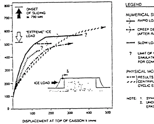
GCRI’s consultants made several predictions of stability and displacements under ice loading using finite element together with centrifuge model testing at 1/125 scale. The finite element work used the ‘ABAQUS’ code and a ‘Modified Critical State’ soil model to represent the sand. Although limited information on the analyses undertaken by GCRI is available, the results with respect to displacements are summarized in figures taken from Jefferies et al, 1985. (see figures 6 and 7 below).
Figure 6: From Jefferies et al, 1985. • Hicks & Smith (1988)
This is the most commonly referenced public analysis of the April 12th ice loading event. It is a two dimensional model that treats the loaded face as a wall. It
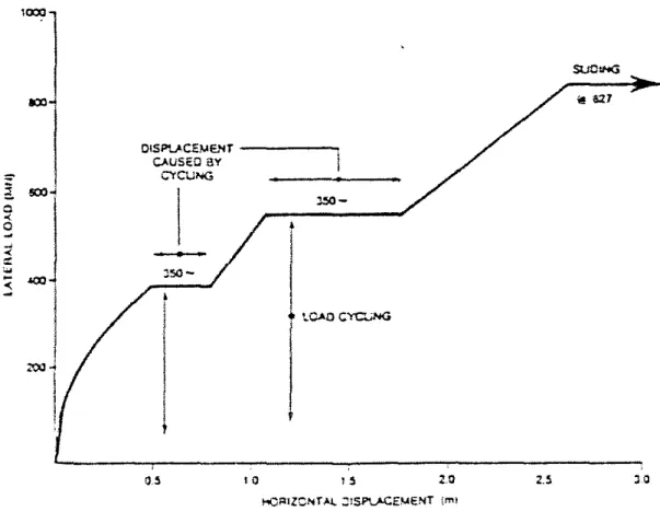
Figure 7: Centrifuge Test Results from Jefferies et al, 1985.
predicts global responses and deformations and does not replicate the Molikpaq as a ring. Therefore predicted deformations can really only be compared with deformations derived from slope indicators.
With respect to their assumption of the core sand density, it is only stated in their paper that ‘They considered their sand density conditions ‘A-B’ to be the closest to those in the field’. Further investigation (Hicks & Smith, 1990) reveals that they assumed the core sand was of medium density (in a dilatant state). This is in contrast to all basic evidence, as explained previously, that the core sand was in a loose state.
• Altaee & Fellenius (1994)
This model is similar to the Hicks & Smith model in that it is a two dimensional model and does not replicate the Molikpaq as a ring. It also includes cyclic loading of the caisson.
With respect to their assumption of the core sand density, it is stated that ‘They consider their soil density conditions C5 are the most representative of the field
conditions.’ In their paper they state that the data on the sand density was specified by Gulf Canada Resources. Referring to figure 1-6 from the C-CORE report (C-CORE, 2008), C5 conditions correspond to an upsilon value of -0.025 (see figure 8).
Figure 8, Caisson cyclic load-displacement response, Altaee & Fellenius (1994) (Figure 1-6 from C-CORE, 2008)
Upsilon values represent the specified initial void ratio differences to the steady state line. These values are basically equivalent to the ‘state parameter’ term used by Been & Jefferies, 1985. An upsilon value of -0.025 corresponds to a dilatant sand. A value of +0.025 or higher would correspond to a contractive sand. Again, the assumptions made by Altaee & Fellenius with respect to the state of the sand are in contrast to all basic evidence, as explained previously, that the core sand was in a loose state.
• Jeyatharan (1991)
This model is similar to the previous two models in that it is a two dimensional model and does not replicate the Molikpaq as a ring. However the focus of the analyses in this case was to predict the excess pore pressure generation and the resulting partial liquefaction and loss of core sand which was observed during the April 12th event.
In the C-CORE report (C-CORE, 2008) it is not specifically stated as to what density was assumed by Jeyatharan for the core sand. However, it can be deduced that the density was assumed to be medium dense because the initial finite element analyses matched with those of Hicks & Smith.
Sandwell Structural Model / Extensometer Calibration for Ice Load Measurement
Sandwell initially analyzed the Molikpaq during the design process in 1981 using the mainframe STARDYNE structural analysis package. In 1988 Sandwell undertook verifications of the original model and the enhancements in modeling which had been incorporated over the ensuing years. This mainframe model was subsequently converted in 1990 to the COSMOS/M structural analysis package for ease of execution. The purpose of the conversion was to have the ability to investigate the response of the structure to a variety of ice loading levels and boundary conditions (load cases). The Sandwell, 1991 report (Extensometer Calibration for Ice Load Measurement) describes this model conversion and the subsequent investigations.
There are a number of assumptions that are made as part of a finite element analysis of specific loads on the Molikpaq using structural computer models. These are outlined in the Sandwell report. Three general assumptions require comment.
Base Shear
As a starting point, Sandwell assumed that 40% of the resistance was generated by base shear. Of the 24 cases that they ran, 15 cases assumed a value of 40%; another 7 cases assumed values greater than 40% and 2 cases assumed a value of 20%. The resistance was modeled as a force on the base of the caisson and it was assumed that strain compatibility required that the base friction be mobilized before the sand core resisted significant loads.
The above assumptions with respect to base shear introduce errors into the analyses for the following reasons.
Strain compatibility dictates that up until the ice load exceeds the sliding resistance of the base of the Molikpaq on the berm, the majority of the load is transferred down into the steel base. Therefore, in reality it is not until the ice load reaches close to the ultimate capacity of the composite structure that the majority of the load, in the order of 75% at that point, is transferred to the core.
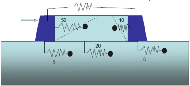
Figure 9, taken from the C-CORE report (C-CORE, 2008) illustrates this process. It shows typical relative displacements to fully mobilize the resistance components of the composite unit. However, based on the
geotechnical models discussed in the next section of this report, a displacement significantly greater than 500mm is most likely required to fully mobilize the passive resistance of the core. Likewise a displacement greater than 50mm is most likely required to fully mobilize the interface friction between the caisson and the berm. In other words if the displacement numbers were ten times or so (in mm) those shown in figure 9 they would be representative of the Molikpaq.
Figure 9: Typical relative displacements (C-CORE, 2008)
The following values are tabled for illustration purposes only (further discussion on the best estimate of the coefficient of friction of the base on the berm is provided later in this report). The sliding resistance of the base of the Molikpaq on the berm can be assumed to be in the order of 200 MN. This value assumes the net weight of the Molikpaq structure is 380 MN and the coefficient of friction of the base on the berm is around 0.5. Likewise the net weight of the core is in the order of 1000 MN with a coefficient of friction of around 0.6 for a sliding resistance in the order of 600 MN. The ultimate resistance is therefore in the order of 800 MN which is consistent with published design predictions.
Based on the above, and assuming that the caisson is not flexible, it can be deduced that for loads up to around 200 MN it is likely that around 90% of the load will be transferred to the base. For loads in the order of 400 MN the percentage will be around 50%, dropping to 33% at 600 MN and 25% at 800 MN. In other words, depending on the load level, the percentage of the load transferred to the base will vary. It is not a fixed
If the caisson is treated as a flexible structure, as it is in the Sandwell analyses, it becomes more complex to estimate the percentage of the load which is transferred to the base for any load. That is because some passive resistance will be mobilized as the structure flexes well before the ultimate sliding resistance of the base of the Molikpaq is achieved.
In summary the percentage of the resistance generated by base shear is a variable, decreasing as the load increases, and the actual percentage at any load is difficult to assess exactly. So choosing a particular value introduces a certain error in the analyses.
Soil Properties (Amauligak I-65 and F-24)
Sandwell conducted analyses for two Amauligak sites (I-65 in 1985/86 and F-24 in 1987/88). For both deployments Sandwell state that they assumed the core sand to be dense cohesionless soil with a dry density of 18 kN/m3 and with a density below water of 10 kN/m3. In fact, of the 24 cases that Sandwell analyzed, they state that 20 assumed soil spring values corresponding to dense sand and 4 assumed soil spring values twice these values. However, as explained below, values actually used for soil stiffnesses in the analyses do not reflect this.
Sandwell’s stated assumption for the core sand would be wrong for both deployments, but especially so for the I-65 deployment which was not densified in any way. As discussed previously, the state of the core sand at Amauligak I-65 was most likely loose. The core sand at F-24 was densified using explosives. This resulted in the core sand having a state toward the loose side of medium dense as it was still less dense than the hopper dumped berm sand.
The implications of the stated assumptions made by Sandwell regarding the density of the core sand and the soil spring values are potentially very significant. The relatively high soil spring values associated with dense sand would result in an over overestimation of ice loads. However this effect would not be as marked for low loads when the base friction component of the resistance is greater.
In an attempt to estimate the implications of Sandwell’s assumptions, soil spring values were investigated by the author. Core soil spring properties used in the analyses are tabled in the Sandwell report. For the I-65 case, the core is assumed to provide a resistance of approximately 31 MN per metre width per metre of deflection. The inside flat face of the Molikpaq, the face pushing directly on the core sand, is 52.5 metres wide. Therefore for a 1 metre horizontal displacement of a rigid caisson the core would provide a resistance of approximately 1,600 MN.
As the core has a depth of 20 metres the corresponding stiffness modulus is approximately 1.5 MPa/m. A review of typical or suggested values for lateral moduli of subgrade reaction indicated that such a value (1.5 MPa/m) would correspond to a loose sand.
In summary, although Sandwell state that they assumed soil spring values corresponding to dense sand, it is the author’s opinion that the soil spring values actually used were probably representative of looser material.
Dewatering and Setdown Elevations, etc.
Other differences relate to the amount of dewatering in the core (depth to the water table) and the setdown elevations. Sandwell ran 8 load cases which were supposedly representative of the Amauligak I-65 deployment and 15 load cases supposedly representative of the F-24 deployment. Although the setdown elevations appear to be very similar, different water table levels (drawdowns) in the core were assumed for the two deployments; -1.5m for I-65 and what appears to be -9.5m for F-24. Based on these assumptions, the two analyses cannot be directly compared.
Sandwell state that the properties for the F-24 analyses were based on the previous mainframe analysis for the F-24 site, and the properties for the I-65 analyses were based on the I-65 deployment. For two reasons it is clear that the F-24 analyses did not represent the actual deployment. At the I-65 site the top of the berm was at -19.5m whereas at the F-24 site was at -15.8m. This is not accounted for in the Sandwell analyses. However for current purposes (the review of loading events at I-65) this erroneous assumption is not relevant. Secondly the author understands that the actual dewatering process was a lot less effective than anticipated and only a nominal reduction in the water table was achieved at both sites. The drawdown value of -9.5m is consistent with the original design assumption of about 10m (Bruce and Harrington, 1982) and it is the author’s understanding that such a drawdown was never achieved.
In summary, although the Sandwell model was calibrated against the original mainframe structural analyses of the Molikpaq and the comparison between the two models was good, some assumptions were made regarding the characteristics of the composite unit and the sand core which were either approximations or not correct. However it is the author’s opinion that none of the assumptions made by Sandwell would result in significant errors and the net effect of these assumptions is likely small.
PERFORMANCE PREDICTIONS Geotechnical Models
• EBA FEM Model
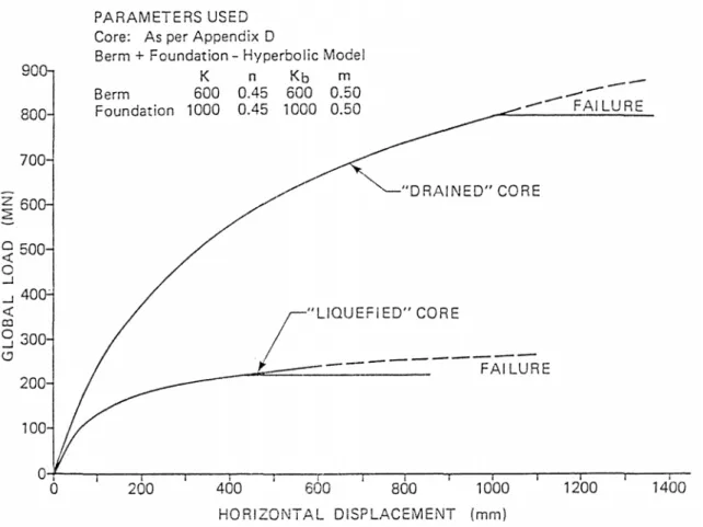
Figure 10, from EBA’s report shows the predicted load displacement relationship for static loading (“Drained Core”). However, as noted previously, the analyses simply treated the caisson and core as an equivalent mass of sand with the caisson acting as a containment membrane. The figure therefore does not reflect the actual load displacement relationships at low displacements when the majority of the load is likely being resisted by caisson base friction.
It is noted in the EBA report that the load displacement relationship is based on ‘best estimate’ parameters. However predicted lateral deformations under static loading are not particularly sensitive to soil parameters within their likely range of values (for a particular sand state). Errors due to estimation of soil parameters are typically of the order of +/- 25 percent in terms of displacement.
The development of the ultimate resistance to static horizontal load on the Molikpaq is complicated. If it were assumed that the critical failure mode were simple truncation at the structure/berm and core/berm interface and for a net structure weight of 380 MN, the ultimate resistance can be simply calculated as about 900 MN. The actual critical failure mode is likely more complicated and probably involves a failure surface that extends up into the core (passive failure). On this assumption simple calculations suggest an ultimate lateral resistance to static loading of about 800 MN. EBA’s load displacement curve matches well with this 800 MN value.
From a limit states perspective, under dynamic horizontal ice loading the ultimate resistance of the Molikpaq is considerably reduced from the static loading case, which assumes no excess pore pressure in the core sand. Because the state of the sand has been assessed as being contractive at high strains, under repetitive loading or very rapid loading, liquefaction of the core could be anticipated. In this situation, according to EBA, the undrained steady state shear strength would be very low, less than about 2kPa. However, as the base of the structure is in direct contact with the berm, which has been assessed as being slightly dilative, the drained shear strength would govern the structure/berm interface strength.
Thus an estimate of the minimum ultimate resistance to ice loading, if the rate and magnitude of loading were sufficient to cause liquefaction of the core, is provided by the sliding resistance of the structure. This was simply calculated by EBA to be about 200 MN.
Again, however, as noted at the beginning of this section, the figure does not reflect the actual load displacement relationships at low displacements when the majority of the load is likely being resisted by caisson base friction. Therefore the shape of this curve at low displacements is not considered representative.
• Gulf Canada Resources Inc. (GCRI) Models
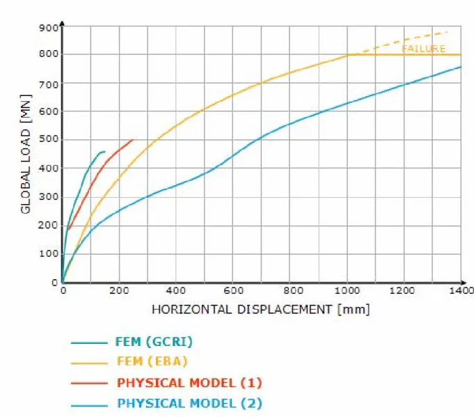
Figures 6 and 7 from Jefferies et al, 1985, show the predicted load displacement relationships for a number of models (both numerical and physical) based on different soil input parameters. Unfortunately the actual differences in the soil input parameters are not well defined in the paper. However several conclusions can be drawn with respect to the soil parameters used in the models.
Three centrifuge model tests were performed. The results for the first two, which are very similar, are depicted in figure 6. The density of the sand in these tests is not defined. However the density of the core sand in the third test, with the results shown on figure 7, is defined as loose. When the three sets of results are drawn to the same scale (with the first two tests combined as physical model #1 and the third test depicted as physical model test #2 - with the cyclic portion of the third test removed) it is very evident that the curve for the loose sand is markedly different to the curves for the other two tests (see figure 11). Because
of this marked difference in the curves, and because it is stated in the paper that the Molikpaq was intended to have a core and berm whose properties correspond to a sand with a state parameter of -0.1 (medium dense to dense sand), it can be deduced that the first two tests were conducted using medium dense to dense sand.
Figure 11: Predicted Horizontal Displacement at Point of Load Application It is also stated in the paper that the deflection behaviours of the two different methods (FEM and centrifuge tests) shown in figure 6 are similar. Inherent in this statement is that the soil parameters in both models were similar (medium dense to dense).
The results of the GCRI FEM analysis are also shown in figure 11 together with the EBA curve, which assumes the core sand to have a density on the border
between loose and medium dense. It can be seen that the trend in the curves is very much as one would anticipate based on the trend in the assumed core sand densities.
Figure 2, from Jefferies et al, 1985 shows the Molikpaq lateral resistance envelope as a function of the core sand’s characteristic state parameter. This envelope is based on GCRI’s finite element results and limit state calculations. As noted previously, Jefferies et al, 1985 point out that ‘significant performance
shortfalls should be expected if the characteristic state of the core sand is looser than zero’ (i.e. if the relative density is less than about 50%). Specifically this
figure shows that under pulsed ice loading the horizontal resistance is very low if the state of the core sand tends toward being loose. Figure 7 also shows that even in a non liquefiable scenario (i.e. under slow repetitive loading) very significant displacements would be anticipated.
• Hicks & Smith (1988)
In Hicks & Smith, 1990 they state that if the core sand was not of medium density then the deformations during the April 12th event (when they understood the global ice load was in the order of 500 MN) would have been uncontrolled! The researchers felt their assumed ice load was justified as they believed it was consistent with precedent and that there were 254 strain gauges and numerous other instrumentation in operation during the April 12th event (This contrasts with the fact that there was no precedent for such a load and there was only ONE strain gauge operational during the critical portion of the event).
• Altaee & Fellenius (1994)
It is stated by C-CORE that Altaee & Fellenius’s static caisson load displacement response was similar to that of Hicks and Smith which is not surprising as they both assumed a medium dense sand in the core.
Their cyclic analyses are more revealing. As can be seen in figure 8, if the core sand were assumed to have an upsilon value of 0.000 (C1), which is only slightly less dense than their assumption, then the required number of cycles to produce major deformations drops very significantly! They state in their paper that ‘The computation results indicate that Case C1, having the loosest sand, would not have been stable for the imposed ice loading.’ Further, had they assumed a more realistic upsilon value of at least +0.025 then a lot lower ice load would produce the same result, which would also result in significant deformations and pore pressure generation.
• Jeyatharan (1991)
It is stated that their initial finite element analyses matched with those of Hicks & Smith. Also in Jeyatharan’s summary he states that ‘Although the (centrifuge)
tests were able to show in a model a pattern of excess pore pressure generation similar to that observed in the field event, they were unable to resolve the controversy about the nature of the loss of sand.’
It is the author’s belief that the loss of sand could be easily replicated if the centrifuge tests were conducted with the core sand in a loose state.
Summary of Geotechnical models
All of the finite element models discussed above appear to be technically sound and the author believes that, within their limits, could be useful tools in predicting field behaviour. However, this would only be true if the input parameters with respect to the insitu state of the sand were correct.
The prior discussions showed that the majority of the FEM analyses and physical model tests assumed that the insitu state of the core sand was medium dense to dense. This is in contrast to all basic evidence that the core sand was in a loose state. The exceptions were the centrifuge model tests depicted in figure 7 where the sand is defined as loose, and the EBA analyses which assume a core density on the border between loose and medium dense (relative density in the order of 35%).
With respect to the three research analyses (Hicks & Smith, 1988; Altaee & Fellenius, 1994; and Jeyatharan, 1991) it is unfortunate that this incorrect assumption with respect to density was made as it appears that the models would likely have predicted the actual performance well. The only adjustment required would be to apply a realistic ice load. Stated another way, if one begins by incorrectly assuming that the core sand was not loose, the conclusion is that the ice loads are high. The converse also holds.
The author finds it quite remarkable and unfortunate that none of these researchers questioned the information given to them by Gulf. The researchers probably cannot be blamed as they were not given access to the raw field data (for confidentiality reasons) to evaluate their work. Further, they appear to have been led to believe that the input parameters were indisputable!
Best Estimate Geotechnical Model
The only predicted load displacement relationship which is based on the assumption of a core density in the range of loose to medium dense (equivalent to a relative density of 35%) is the EBA relationship. The relationship appears reasonable when compared with other relationships based on other density assumptions (see figure 11). Also the model and analyses are reasonably well documented (Sladen & Hayley, 1988). However, similar to all the other geotechnical models, the FEM mesh did not incorporate the structural properties
of the caisson; it simply treated the caisson and core as an equivalent mass of sand with the caisson acting as a containment membrane.
As mentioned previously, this simplification was perfectly adequate for the intended purpose at the time, which was to predict the performance of the composite unit under large dynamic loads. However to model the stress/strain behaviour at low loads requires consideration of the relative load sharing between the caisson and the core. As discussed in the section on the Sandwell model, in order to satisfy strain compatibility under relatively low loading the majority of load is transferred down into the caisson base.
To develop a stress/strain relationship for low loads requires a best estimate of the base friction angle (sand – steel friction). The most appropriate angle to use is not easy to define as it is function of a number of factors including the density of the sand at the interface and the roughness of the base, which is unknown to the author. During the design and evaluation of the Molikpaq numerous values were assumed ranging from about 10 degrees up to 27 degrees. The corresponding coefficients of friction are approximately 0.18 and 0.5, which is a considerable range.
It can be assumed that the surface of the berm consisted of loose sand as a result of the leveling process (raking with the draghead). According to API 2A (Recommended Practice for Planning, Designing and Constructing Fixed Offshore Platforms) the design soil-pile friction angle for steel piles in loose sand is 20 degrees. So for current purposes this angle will be used as a best estimate. The coefficient of friction for 20 degrees is 0.364. Assuming the caisson weighs 380 MN, the ultimate frictional force is 138 MN.
To mobilize this force would require a movement in the order of 50mm (see previous discussion). At this amount of displacement the EBA curve shows that some passive resistance is mobilized. However the actual passive resistance will be somewhat less than calculated by EBA as part of their ‘core’ is replaced by the caisson. Based on these assumptions a new curve has been developed (see figure 12).
This curve shows that for a core displacement of 50mm the global load would be around 240 MN. At 100mm of core displacement this load would be close to 300 MN.
Figure 12: Author’s ‘Best Estimate’ Load Displacement (based primarily on Sladen & Hayley, 1988) Sandwell Structural Model
A total of 23 load cases were run: 15 for the Amauligak F-24 site and 8 for the I-65 site. Although, as noted previously, the cases considered did not actually represent actual situations the results provide indications of the effects of different input parameters and assumptions. Details of the results of these load cases are provided in the Sandwell report.
The output from the analyses was the global deformation of the structure under various ice loads. The key output parameter was the North – South deflection of the structure as a function of the ice load in MN/mm (i.e. the load distortion ratio in the direction of the ice load).
To quote the Sandwell report, ‘The main observation made was that the
North-South load distortion ratio using the Face Load component was in the range of 2.0 to 4.2 MN/mm (the average is actually 2.76), which was approximately half the field data estimate of 6 MN/mm at low load levels. This would indicate that the actual structure and soil interaction is much stiffer than the model or that the application of the ice load is lower or that base shear is more significant than assumed etc. Clearly the calculated load distortion ratios do not compare well to
field data measurements.’ (Ice loads, based on Medof panel data, and the
corresponding extensometer readings were supplied to Sandwell by GCRI). The most obvious conclusion, which Sandwell have not made mention of, is that the ice loads supplied to them (the field data) were incorrect (too high).
Considering the load distortion ratios for the eleven most likely scenarios, it can be seen that they varied from 2.2 to 3.3 MN/mm with an average of 2.84 MN/mm. The implication of the combination of the assumptions made by Sandwell is difficult to quantify without resurrecting the original COSMOS/M analyses and inputting appropriate values. However it is the author’s opinion, as discussed previously, that none of the assumptions made by Sandwell would result in significant errors and the net effect of these assumptions is likely small.
MEASURED DISPLACEMENTS General
As mentioned previously, there is a very important difference between the pure geotechnical models and the Sandwell model and this has to be fully appreciated. To estimate ice loads using the geotechnical models requires good slope indicator data. The Sandwell model requires extensometer readings to estimate ice loads.
Slope Indicators
A total of seven slope indicator (SI) casings were installed as part of the Amauligak I-65 monitoring program. The location and numbering of the casings is shown on the following schematic figure 13.
A A I01 I02 I03 I04 I05 I06 I07 Conductor Pipe A-A Conductor Pipe I04 I01 I06
Sensor
Wheels
Lateral deformations were measured by profiling each casing with the downhole SI probe. When compared with previous readings, any zones of net or ‘plastic’ deformation could be identified and then correlated with ice events during that period.
According to Gulf Canada Resources (Dynamic Horizontal Ice Loading on an Offshore Structure, Phase 1A: Molikpaq Performance at Amauligak I-65, Volume VIII of X, Geotechnical Monitoring), significant deformations only occurred in some or all of the casings due to ice events on March 7/8, April 12 and May 12, 1986. The table 2 summarizes the lateral deformations in the seven inclinometer casings as a result of the three events, as interpreted by Gulf Canada Resources. Also shown in table 2 are the ice loads for each event as estimated by Gulf at the time. It was noted by Gulf that all displacements shown in the table occurred at the interface of the bottom of the core and the berm and above (within the core itself).
Events Summary Lateral Displacement [mm] toward: Event Date GCRI Estimated load [MN] Ice load towards: I01 N I02 NE I03 W I04 C I05 E I06 S I07 SW March 7/8 300 East, SE, South 12 S 16 SE 8 N * 20 E * 12 NW April 12 500 West, NW 18 NW 28 N 24 N 12 W ** 30 SW 16 W May 12 200 South 14 S 14 S 0 0 0 0 0
* Casing not profiled for this event ** Casing sheared in core during event
Highlighted events are discussed in the following pages.
Table 2: Lateral deformations as interpreted by Gulf Canada Resources. Two strings of in-place inclinometers (IPI’s) were located in SI casings I-01 North and I-06 South. Comparison of SI data and IPI data were made by Gulf. Correlation coefficients ranged from -0.58 to 0.76 indicating in the best case only marginal correlation between the two sensors.
The author has undertaken his own review of all the SI profiles for the three events and compared the interpretations with those presented by Gulf. In summary the two interpretations do not match for most profiles, both with respect to displacements and direction. Four sets of profiles are included in figures 14 – 17 to illustrate the difficulty in interpretation.
Figure 14. Inclinometer I01 (north) for the March 7/8 event
With respect to Inclinometer I01 (north) for the March 7/8 event, according to table 2 the lateral displacement was 12mm to the south and the direction of the ice load was generally to the south-east. According to figure 14, the direction of the resultant lateral displacement varied with depth and at full depth was to the north –west. The displacement from the base of the core was approximately 16mm. In other words, according to the figure, the resultant displacement was in the opposite direction to the load. The settlement of the core at this location during this event was approximately 15mm.
Figure 15. Inclinometer I03 (west) for the March 7/8 event
With respect to Inclinometer I03 (west) for the March 7/8 event, according to table 2 the lateral displacement was 8mm to the north and the direction of the ice load was generally to the south-east. A review of the figure shows that there is no discernable trend of displacement or direction. As the northern settlement plate recorded a settlement of 15mm during this event, this location most likely also experienced settlement of the same order.
Figure 16. Inclinometer I03 (west) for the April 12th event
With respect to Inclinometer I03 (west) for the April 12th event, according to table 2 the lateral displacement was 24mm to the north and the direction of the ice load was generally to the west. A review of the figure shows that the displacement in the core was 12mm to the west. This location experienced a settlement between 7 and 14mm (depending on which data source is used).
Figure 17. Inclinometer I04 (centre) for the April 12th event
With respect to Inclinometer I04 (centre) for the April 12th event, according to table 2 the lateral displacement was 12mm to the west and the direction of the ice load was generally to the west. A review of the figure shows that there is a linear bias in the resultant deflection plot from the point of fixity. There is no discernable trend of displacement or direction. There were a few milimetres of settlement at this location during this event.
It should also be noted that when the maximum displacement of 30mm was recorded at inclinometer I06 (south) for the April 12th event, the casing experienced a settlement of almost twice this amount.
Based on the review of all the inclinometer profiles the author provides the following comments:
• The quoted values and directions in the Gulf Canada Resources table (table 2) are generally not consistent with the actual profiles.
• The trend in the direction of the displacements is actually toward the perimeter of the caisson as opposed to in the direction of the ice load. • All three events were dynamic and as a result the sand around the
inclinometers settled during these events, in some cases by very large amounts (see figures 18 and 19 which show accelerations during the April 12th event and the subsequent settlements of the core and the caisson). • The minor settlements would explain the random scatter in the direction
and amount of displacement in many of the profiles. This scatter is consistent with there being no correlation between the SI and IPI data. • The large settlements (slumping) would explain the trend in the direction
of the displacements toward the perimeter of the caisson. • The centre inclinometer showed no displacement.
2%g
2.5%g
3.5%g
3.5%g
8.5%g
>11%g
4.5%g
Figure 18: Accelerations during the April 12th event
The author’s conclusion is that if there was any permanent displacement of the Molikpaq in the direction of the ice load it would have been small and would not have been discernable from the inclinometer data. The settlements of the sand during the three significant ice events negate meaningful interpretation of displacements by means of inclinometers.
+1 -13 -34 -44 -19 -2 +2 +5 -1,310 -50 -7 -7 -76 -3
Figure 19: Settlements after April 12th event (mm)
(Core settlements in white letters, caisson settlements in yellow letters) (Note that the loaded caisson face settled as opposed to rising) Extensometers
The extensometers measure the deflection of the caisson relative to the central conductor casing that is assumed to be fixed. The following schematic figure 20 shows the location of the extensometers (in pink).
The author has conducted his own review of the maximum extensometer readings for the five significant events in 1986. These values are shown in table 3.
DATE MAXIMUM EXTENSOMETER DEFLECTION (mm) 8th March 37 25th March 20 12th April AM 60 12th April PM 30 12th May 45
Table 3: Maximum extensometer readings for the five significant events in 1986
ICE LOAD ESTIMATES Using Geotechnical models
As mentioned previously, all the geotechnical models only consider the response of the sand in the core and the berm. The only means of measuring these global deformations is by slope indicators. However it has previously been concluded in this report that the settlements of the sand during the three significant ice events negate meaningful interpretation of displacements by means of inclinometers. It was concluded that if there was any permanent displacement of the Molikpaq in the direction of the ice load it would have been small and could not be quantified from the inclinometer data.
It is well realized that other reviewers of the slope indicator data may choose to reach a different conclusion. Because of this possibility the author has investigated the consequences of choosing the worst case scenario whereby it is assumed that the slope indicator data is not only real, but the tabled displacements are also in the direction of the ice load. From the table provided by GCRI (table 2) the maximum deflections for the three significant events, March 7/8, April 12 and May 12, 1986 are respectively 20mm, 30mm and 14mm. These displacements are residual (non recoverable) displacements. Knowing that the events were dynamic (involving numerous cycles of loading) and the core sand was loose, it is likely that these residual displacements represent a significant portion of the ‘elastic’ displacement. However, again to be extremely conservative, let us assume that the residual displacements were one third of the ’elastic’ displacements.
Based on the above, the most extreme estimates of maximum displacements for the three events are 60mm, 90mm and 42mm. To interpret ice loads from these deflections, we will use the ‘best estimate’ geotechnical curve (Figure 12). Assuming fully drained conditions, another conservatism, the corresponding