HAL Id: hal-02875476
https://hal.archives-ouvertes.fr/hal-02875476
Submitted on 19 Jun 2020
HAL is a multi-disciplinary open access
archive for the deposit and dissemination of
sci-entific research documents, whether they are
pub-lished or not. The documents may come from
teaching and research institutions in France or
abroad, or from public or private research centers.
L’archive ouverte pluridisciplinaire HAL, est
destinée au dépôt et à la diffusion de documents
scientifiques de niveau recherche, publiés ou non,
émanant des établissements d’enseignement et de
recherche français ou étrangers, des laboratoires
publics ou privés.
multi-model evaluation
Maria Sand, Bjørn Samset, Yves Balkanski, Susanne Bauer, Nicolas Bellouin,
Terje Berntsen, Huisheng Bian, Mian Chin, Thomas Diehl, Richard Easter, et
al.
To cite this version:
Maria Sand, Bjørn Samset, Yves Balkanski, Susanne Bauer, Nicolas Bellouin, et al.. Aerosols at the
poles: an AeroCom Phase II multi-model evaluation. Atmospheric Chemistry and Physics, European
Geosciences Union, 2017, 17, pp.12197 - 12218. �10.5194/acp-17-12197-2017�. �hal-02875476�
https://doi.org/10.5194/acp-17-12197-2017 © Author(s) 2017. This work is distributed under the Creative Commons Attribution 3.0 License.
Aerosols at the poles: an AeroCom Phase II multi-model evaluation
Maria Sand1,2, Bjørn H. Samset1, Yves Balkanski3, Susanne Bauer2, Nicolas Bellouin4, Terje K. Berntsen1,5, Huisheng Bian6, Mian Chin7, Thomas Diehl8, Richard Easter9, Steven J. Ghan9, Trond Iversen10, Alf Kirkevåg10, Jean-François Lamarque11, Guangxing Lin9, Xiaohong Liu12, Gan Luo13, Gunnar Myhre1, Twan van Noije14, Joyce E. Penner15, Michael Schulz10, Øyvind Seland10, Ragnhild B. Skeie1, Philip Stier16, Toshihiko Takemura17, Kostas Tsigaridis2, Fangqun Yu13, Kai Zhang18,9, and Hua Zhang19
1Center for International Climate and Environmental Research – Oslo (CICERO), Oslo, Norway 2NASA Goddard Institute for Space Studies and Columbia Earth Institute, New York, NY, USA
3Laboratoire des Sciences du Climat et de l’Environnement, CEA-CNRS-UVSQ, Gif-sur-Yvette, France 4Department of Meteorology, University of Reading, Reading, UK
5Department of Geosciences, University of Oslo, Oslo, Norway
6Earth System Science Interdisciplinary Center, University of Maryland, College Park, MD, USA 7NASA Goddard Space Flight Center, Greenbelt, MD, USA
8Directorate for Sustainable Resources, Joint Research Centre, European Commission, Ispra, Italy 9Pacific Northwest National Laboratory, Richland, WA, USA
10Norwegian Meteorological Institute, Oslo, Norway
11National Center for Atmospheric Research, Boulder, CO, USA 12Department of Atmospheric Science, University of Wyoming, USA
13Atmospheric Sciences Research Center, State University of New York at Albany, New York, USA 14Royal Netherlands Meteorological Institute, De Bilt, the Netherlands
15Climate and Space Sciences and Engineering, University of Michigan, Ann Arbor, MI, USA 16Department of Physics, University of Oxford, Oxford, UK
17Research Institute for Applied Mechanics, Kyushu University, Fukuoka, Japan 18Max Planck Institute for Meteorology, Hamburg, Germany
19Laboratory for Climate Studies, National Climate Center, China Meteorological Administration, Beijing, China
Correspondence to:Maria Sand (maria.sand@cicero.oslo.no) Received: 13 December 2016 – Discussion started: 10 February 2017
Revised: 23 August 2017 – Accepted: 24 August 2017 – Published: 13 October 2017
Abstract. Atmospheric aerosols from anthropogenic and natural sources reach the polar regions through long-range transport and affect the local radiation balance. Such trans-port is, however, poorly constrained in present-day global climate models, and few multi-model evaluations of polar an-thropogenic aerosol radiative forcing exist. Here we compare the aerosol optical depth (AOD) at 550 nm from simulations with 16 global aerosol models from the AeroCom Phase II model intercomparison project with available observations at both poles. We show that the annual mean multi-model me-dian is representative of the observations in Arctic, but that the intermodel spread is large. We also document the geo-graphical distribution and seasonal cycle of the AOD for the
individual aerosol species: black carbon (BC) from fossil fuel and biomass burning, sulfate, organic aerosols (OAs), dust, and sea-salt. For a subset of models that represent nitrate and secondary organic aerosols (SOAs), we document the role of these aerosols at high latitudes.
The seasonal dependence of natural and anthropogenic aerosols differs with natural aerosols peaking in winter (sea-salt) and spring (dust), whereas AOD from anthropogenic aerosols peaks in late spring and summer. The models pro-duce a median annual mean AOD of 0.07 in the Arctic (de-fined here as north of 60◦N). The models also predict a note-worthy aerosol transport to the Antarctic (south of 70◦S) with a resulting AOD varying between 0.01 and 0.02. The
models have estimated the shortwave anthropogenic radia-tive forcing contributions to the direct aerosol effect (DAE) associated with BC and OA from fossil fuel and biofuel (FF), sulfate, SOAs, nitrate, and biomass burning from BC and OA emissions combined. The Arctic modelled annual mean DAE is slightly negative (−0.12 W m−2), dominated by a positive BC FF DAE in spring and a negative sulfate DAE in sum-mer. The Antarctic DAE is governed by BC FF. We per-form sensitivity experiments with one of the AeroCom mod-els (GISS modelE) to investigate how regional emissions of BC and sulfate and the lifetime of BC influence the Arctic and Antarctic AOD. A doubling of emissions in eastern Asia results in a 33 % increase in Arctic AOD of BC. A doubling of the BC lifetime results in a 39 % increase in Arctic AOD of BC. However, these radical changes still fall within the AeroCom model range.
1 Introduction
The polar regions are relatively free from local sources of an-thropogenic climate drivers, but are still experiencing rapid changes to increasing greenhouse gas concentrations, which are distributed globally. These changes are amplified by feed-backs in the system, such as temperature feedfeed-backs and the ice albedo feedback (Pithan and Mauritsen, 2014). The tem-perature in the Arctic is experiencing increases that are twice the global rate, resulting in reductions in summer sea-ice (Hartmann et al., 2013; Screen and Simmonds, 2010). In the Antarctic, summer sea-ice is increasing, while several inte-rior regions are rapidly losing ice mass (Rignot et al., 2008). The role of aerosols in the ongoing polar climate changes is not well understood. Yang et al. (2014) emphasize the im-portance of including aerosols in models when simulating the recent changes in the Arctic climate. For instance, the measured decrease in anthropogenic sulfate concentrations in the Arctic over the last decades (Hirdman et al., 2010; Quinn et al., 2009) may have had a warming effect on the Arctic (Navarro et al., 2016). Shindell and Faluvegi (2009) showed that decreasing sulfate and increasing BC concentra-tions over the last three decades have substantially warmed the Arctic. In general, the climate impacts of aerosols and clouds constitute one of the largest sources of uncertainty in climate models (Boucher et al., 2013). This is true on a global scale and likely for the critical polar regions, where both sensitivities and dynamical processes may differ signif-icantly from global mean values. Reducing these uncertain-ties is crucial for improving the reliability of future climate projections.
Aerosols perturb the Earth’s radiation balance through ex-tinction of solar radiation (McCormick and Ludwig, 1967; Schulz et al., 2006). By scattering solar radiation, aerosols produce a negative DAE at the top-of-the-atmosphere (TOA). Some aerosols such as BC and dust also absorb solar
radia-tion, and this absorption can lead to a positive DAE TOA (Bond et al., 2013). For a given aerosol abundance, the mag-nitude and sign of the DAE depend on the underlying sur-face albedo (Haywood and Shine, 1995). In the polar regions, the high albedo of snow- and ice-covered surfaces will in-crease the absorption associated with the DAE for absorbing aerosols (Hansen and Nazarenko, 2004; Bond et al., 2013). Concurrently, deposition of BC and dust can reduce the sur-face albedo and promote snowmelt (Flanner et al., 2009; Krinner et al., 2006; Clarke and Noone, 1985). Aerosols also influence the energy balance by changing the optical proper-ties and lifetime of clouds (Twomey, 1977; Albrecht, 1989), and through changes to atmospheric stability (Hansen et al., 1997; Hodnebrog et al., 2014; Samset and Myhre, 2015).
The amount of aerosols emitted into the atmosphere has increased over the industrial era. Myhre et al. (2013) re-ported on the DAE due to anthropogenic aerosols in Aero-Com Phase II. The global model median DAE of the total aerosol effect, taking into account changes to BC, sulfate, OA, biomass burning aerosols, nitrate, and secondary organic aerosols, was estimated at −0.27 W m−2with an intermodel range of −0.58 to −0.02 W m−2for the time period 1850– 2000. Modifying the results from models with missing SOAs and nitrate by use of results from the other models and scal-ing the period to 1750–2010 resulted in a median DAE of −0.35 W m−2.
Most of the aerosols in the polar regions originate from lower latitudes and midlatitudes (Koch and Hansen, 2005; Hirdman et al., 2010). Large-scale planetary circulations in the Northern Hemisphere govern transport into the Arctic. The pronounced seasonal cycle of Arctic AOD typically has a maximum in late winter and spring due to a wintertime build-up in the shallow boundary layer with effective trans-port and reduced scavenging, often referred to as the Arc-tic haze (Iversen and Joranger, 1985; Stohl, 2006). The sea-sonal cycle of Arctic AOD also varies spatially due to chang-ing emissions, composition, and transport patterns. In sprchang-ing, pollution haze and dust plumes from Asian deserts are most common, while late in the season biomass burning and wild-fire smoke from North America and Siberia are observed more frequently (Tomasi et al., 2007). As the Arctic ice melts and more open water is exposed, emissions of sea-salt, dimethylsulfide (DMS), and organic aerosols within the Arctic are expected to increase (Nilsson et al., 2001; Browse et al., 2014).
In the Antarctic, sea-salt particles dominate the coastal sites, which are strongly influenced by the surrounding ocean (Tomasi et al., 2007). In summer, the sulfate from DMS pro-duced by phytoplankton is at its peak, which can also influ-ence the aerosol distribution in the Antarctic (Arimoto et al., 2004). The stations on the Antarctic Plateau, conversely, are mostly influenced by long-range transport in the free tropo-sphere and the subsidence of fine sulfate and methane sul-fonic acid (MSA) (Hara et al., 2004; Bigg, 1980; Tomasi et al., 2015). Sea-salt measured here originates mainly from
marine air transported by large storm events. The Antarctic is also influenced by smoke aerosols transported from South America, Australia, and southern Africa (Fiebig et al., 2009; Stohl and Sodemann, 2010).
The ability of climate models to simulate aerosol burdens in remote regions depends on transport and precipitation, as well as internal aerosol physical and chemical parameteriza-tions, such as wet deposition, oxidation, and microphysics (Shindell et al., 2008; Textor et al., 2006; Zhou et al., 2012; von Hardenberg et al., 2012). Aerosol observations in the po-lar regions are sparse. Previous comparisons between models and single observations show significant model biases (Stohl et al., 2013; Shindell et al., 2008; Koch et al., 2009). Eck-hardt et al. (2015) evaluate sulfate and BC concentrations from different models against a large set of ground-based and aircraft measurements in the Arctic. They find that the aerosol seasonal cycle at the surface is weak in most models and that the concentrations of equivalent BC and sulfate are underestimated in winter and spring, but improved relative to earlier comparisons. Jiao et al. (2014) compare AeroCom Phase II models with observations of BC in snow in the Arc-tic. They find that simulated BC distributions in snow are not well correlated with measurements, but that averaged values over the measurement domain are close to observed. The BC atmospheric residence time in the Arctic varies from 3.7 to 23.2 days in the models, and they suggest that aerosol re-moval processes are a leading source of variation in model performance in the Arctic. Kristiansen et al. (2016) calculate the aerosol lifetime by using observations of two radioactive isotopes released from the Fukushima nuclear power plant accident: one passive tracer and one that condenses on sul-fate particles (137Cs) that were used as a proxy for sulfate aerosols’ fate in the atmosphere. Based on surface measure-ments taken in the weeks after the release, they derive an e-folding lifetime of 14.3 days for137Cs, which serves as an estimate of the lifetime of sulfate. They compare this esti-mate with 19 AeroCom Phase II models initialized with the same identical emissions of137Cs and the passive tracer. The AeroCom models show a large spread in their estimates life-times (4.8 to 26.7 days) and a mean of 9.4 days, which is low compared to the measurements (14.3 days). The under-estimation is larger for the northernmost stations, suggesting that the models remove aerosols too quickly and underesti-mate the transport to the Arctic.
Here we present results from Phase II of the AeroCom model experiment. The goal is to document the seasonal cycle of mean aerosol abundances and the resulting DAE at the poles, predicted by climate models presently in use, and the multi-model spread. The DAE does not include indi-rect cloud effects or surface albedo modifications. As global aerosol emissions may change rapidly, both in magnitude and geographical distribution, and aerosol abundance obser-vations in the polar regions are sparse, one aim of the present study is to deliver a baseline to which future model studies and observations may be compared.
2 Methods 2.1 Models
We have used results from 16 global aerosol models that participated in the AeroCom Phase II project (e.g. Myhre et al., 2013) http://aerocom.met.no. The models are NCAR-CAM3.5 (Lamarque et al., 2010, 2012), CAM4-Oslo (Kirkevåg et al., 2013), CAM5.1 (Liu et al., 2012), GISS-MATRIX (Bauer et al., 2008), GISS modelE (Koch et al., 2011), GMI-MERRA-v3 (Bian et al., 2009), GOCART-v4 (Chin et al., 2009), HadGEM2 (Bellouin et al., 2011), IMPACT (Lin et al., 2012), INCA (Szopa et al., 2013), ECHAM5-HAM2 (Stier et al., 2005; Zhang et al., 2012b), OsloCTM2 (Skeie et al., 2011), SPRINTARS (Takemura et al., 2005), TM5 (Vignati et al., 2004), GEOS-Chem (Yu and Luo, 2009), and BCC (Zhang et al., 2012a). Model descriptions including model resolution, meteorology, and aerosol microphysics are given in Table S1 in the Supple-ment.
Each model has provided climate and aerosol simulations using year 2006 meteorology. For present-day simulations emissions for the year 2000 have been used, and for prein-dustrial runs year 1850 emissions have been used (Lamar-que et al., 2010). All AeroCom models include sulfate, BC, primary organic carbon, sea-salt, and mineral dust in their total AOD, and some models also include nitrate and SOA. To report on the individual species, the models have either added double calls to the radiation code (i.e. for each time step the radiation code is called with and without the ar-guments needed to calculate the given species’ forcing) or performed additional runs where each species has been run with preindustrial emissions. However, not all models were able to extract the AOD for the individual species. Table 1 lists the models and the species reported by each model. The individual species include BC (from fossil fuel, bio-fuel, and biomass burning emissions), sulfate, total OA (from fossil fuel, biofuel, and biomass burning emissions), nitrate, SOA, sea-salt, and dust. Here, organic aerosols refer to the total mass of organic compounds in the aerosol (both pri-mary and secondary). For a comprehensive documentation on OA and SOA treatment in the AeroCom Phase II mod-els, see Tsigaridis et al. (2014). The AOD is a measure of the total extinction (scattering and absorption) of sunlight as it passes through the atmosphere. In this study we use the AOD at 550 nm wavelength. The models have estimated AOD as a combination of aerosol abundances and optical properties, which is why AOD can be reported in the months in which there is no actual sunlight. The DAE is calculated as the difference in TOA SW radiation between simulations with present-day and preindustrial emissions of aerosols and their precursors (under all-sky conditions). Results are avail-able for total aerosol forcing, as well as for individual aerosol species (BC from fossil fuel and biofuel emissions (FF), sul-fate, total OA FF, nitrate, SOA, and OA and BC combined
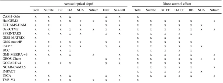
Table 1. List of the models used in this study and which species they have reported.
Aerosol optical depth Direct aerosol effect
Total Sulfate BC OA SOA Nitrate Dust Sea-salt Total Sulfate BC FF OA FF BB SOA Nitrate CAM4-Oslo x x x x x x x HadGEM2 x x x x x x x x x x x x x x ECHAM5-HAM x x x x x x x x x x x x OsloCTM2 x x x x x x x x x x x x x x x SPRINTARS x x x x x x x x x x x x GISS-MATRIX x x x x x GISS-modelE x x x x x x x x x x x x CAM5.1 x x x x x x x x x x x x x BCC x x x x x x x x x GMI-MERRA-v3 x x x x x x x x x x x x GEOS-Chem x x x x x x x x x x GOCART-v4 x x x x x x x x x x x NCAR-CAM3.5 x x x x x x x IMPACT x x x x x x x INCA x x x x x x x x x x x x TM5-V3 x x x x x x x x
Table 2. List of the Arctic and Antarctic stations with ground-based measurements of AOD. Data for Tiksi, Andenes, Yakutsk, Bonanza Creek, Resolute Bay, and Kangerlussuaq are taken from the AERONET database (http://aeronet.gsfc.nasa.gov/) and data from Ny-Ålesund, Barrow, and Alert are from Stone et al. (2014) and Tomasi et al. (2015).
Stations Coordinates and altitude (a.m.s.l.) Measurement period Tiksi 71◦N, 128◦E, Alt 0 m 2010–2012, 2014
Andenes 69◦N, 16◦E, Alt 379 m 2002, 2008–2011, 2013, 2014 Yakutsk 61◦N, 129◦E, Alt 118 m 2004–2015
Bonanza Creek 64◦N, 148◦W, Alt 150 m 1994–1997, 1999–2015 Resolute_Bay 74◦N, 94◦W, Alt 40 m 2004, 2006, 2008–2015 Kangerlussuaq 66◦N, 50◦W, Alt 320 m 2008–2015 Ny-Ålesund 78◦N, 11◦E, Alt 5 m 2001–2011 Barrow 71◦N, 156◦W, Alt 8 m 2001–2011 Alert 82◦N, 62◦W, Alt 210 m 2004–2011 Neumeyer 70◦S, 8◦W, Alt 40 m 2000–2007 Troll 72◦S, 2◦E, Alt 1309 m 2007–2013 South Pole 90◦S, 0◦E, Alt 2835 m 2001–2012
from biomass burning (BB) emissions. Hereafter we will use the term “BC” for total BC (from fossil fuel, biofuel, and biomass burning emissions) and BC FF for anthropogenic BC (from fossil fuel and biofuel emissions), and the same is used for total OA. For AOD we report BC (and OA) only, and for DAE we distinguish between BC FF, OA FF, and biomass burning, the latter consisting of emissions from both BC and OA. For information on the radiative transfer schemes of the individual models, see Stier et al. (2013), their Table 2, and the aerosol model references in Myhre et al. (2013), their Table 2. Uncertainties in calculating the radiative impact of aerosols are linked to the vertical distribution of aerosols (Samset et al., 2013; Kipling et al., 2016). A comparison of the aerosol vertical extinction coefficient from 11 Ae-roCom models to CALIPSO has been performed in Koffi et al. (2016) showing that about half of the models capture the mean aerosol vertical distribution. The models generally
perform better over ocean than land (9 of 11 models repro-duce the aerosol mean vertical distribution over ocean), while the models underestimate the mean aerosol distribution over land. The annual mean multi-model mean absolute error is 11 %, but the bias depends highly on model, season, and re-gion. The negative bias is especially pronounced in spring and summer, in source regions in Africa and Asia dominated by biomass burning (−17 to −26 % bias) and dust (−8 to −23 %).
Even if the models used meteorology for the year 2006, there is some intermodel variability in the simulated wind. Some models are nudged to different sets of reanalysis, while others have used different prescribed meteorology data sets; see Table S1. Three models (NCAR-CAM3.5, CAM4-Oslo, and CAM5.1) have calculated the meteorology online, i.e. with free-running meteorological fields. In CAM4-Oslo the meteorology is calculated based on the CAM4 aerosol
ex-tinction and cloud droplet fields, which do not differ be-tween preindustrial and present-day simulations. The two other models have been run for several years to account for the year-to-year variability, and the reported simulations are based on a 5-year average. The fields (wind, tempera-ture, humidity) are not identical for the preindustrial simu-lations and the present-day simusimu-lations in these two models. The calculated aerosol-induced climate response in the po-lar regions will therefore be due to a combination of differ-ences in emissions and in transport and lifetime. One model (GISS modelE) has duplicate 6-year runs with both nudged winds and free-running winds for preindustrial and present-day conditions, and we find that the difference in the Arctic fraction of the transported tracers between the nudged and the free wind simulations is small. The difference varies be-tween 0.1 and 1.0 % for most species (up to 2.0 % for a few species), for both preindustrial and present-day simulations. Another study with the CAM5.3 MAM4 model finds a sig-nificant difference in BC concentrations on a global scale between nudged and free-running winds (Liu et al., 2016), while the differences between the nudged and unnudged runs in a study with ECHAM-HAM were small (von Hardenberg et al., 2012). Nevertheless, it did not make much difference for the ensemble results as to whether we included or ex-cluded the three models that generated their own winds, and we have therefore decided to include these models in the analysis.
There is no unique definition of the Arctic region and here we have defined the Arctic as the region north of 60◦N, a def-inition found in other studies (Shindell and Faluvegi, 2009; AMAP, 2011). To avoid a large influence from the Southern Ocean we have defined the Antarctic as the region south of 70◦S.
2.2 Comparison with observations 2.2.1 AERONET
We have compared the modelled seasonal cycle of AOD in the grid box of each model in which the respective station is located with ground-based measurements from 12 sta-tions in the Arctic and Antarctic from the AErosol RObotic NETwork (AERONET) http://aeronet.gsfc.nasa.gov/ (Hol-ben et al., 1998). The locations for each station are plotted in Fig. 3, and the coordinates and measurement years for each station are given in Table 2. For Barrow, Alert, and Ny-Ålesund, we have used monthly mean climatology de-rived from daily mean of spectral AOD reported in Stone et al. (2014). For the three stations in Antarctica, one coastal (Neumayer), one mid-altitude (Troll), and one plateau (South Pole) monthly mean climatology are taken from Tomasi et al. (2015).
2.2.2 MODIS
Due to the high reflectance over bright surfaces, obtaining reliable satellite retrieval of AOD is difficult at the poles. Glantz et al. (2014) compared AOD 555 nm from the Mod-erate Resolution Imaging Spectroradiometer (MODIS) Aqua collection 5 Level 2 (Remer et al., 2005) over (dark) ocean areas around Svalbard with available AERONET ground-based measurements at Svalbard (Longyearbyen, 78.2◦N, 15.6◦E; Hornsund, 77.0◦N, 15.6◦E) for the period 2003– 2011. They found comparable values in the summer sea-son (JJA) (0.041 ± 0.025 for MODIS and 0.043 ± 0.024 for AERONET) and early autumn (September) (0.035 ± 0.021 for MODIS and 0.038 ± 0.021 for AERONET), but larger differences in spring (0.115 ± 0.069 for MODIS and 0.093 ± 0.050 for AERONET). The spring differences are partly explained by diverse air masses causing inhomoge-neous aerosol geographical distributions. Glantz et al. (2014) conclude that satellite AOD retrievals in the Arctic marine at-mosphere vary within the expected uncertainties of MODIS retrieval over ocean and can be of use to climate model vali-dation. We have compared the MODIS AOD values with the AeroCom models averaged over the same area (75–82◦N, 10◦W–40◦E), illustrated in Fig. 3 (in blue). For details on the retrieval, see Glantz et al. (2014).
2.2.3 CALIOP
We have compared modelled AOD with retrieved AOD from the Cloud-Aerosol LIdar with Orthogonal Polariza-tion (CALIOP) on board the Cloud–Aerosol Lidar and In-frared Pathfinder Satellite Observations (CALIPSO) satellite (Winker et al., 2013). CALIOP is an active nadir-looking backscattering lidar. It distinguishes clouds and aerosols by using the total backscatter radiation measured at 1063 nm combined with the linear depolarization at 532 nm (Liu et al., 2009). Because it is an active instrument, CALIOP can retrieve aerosol and cloud vertical profiles in the day and at night, and can measure over the highly reflective surfaces in the Arctic. However, daytime retrievals are affected by the noise from scattering of solar radiation and are therefore less accurate than night-time retrievals (Winker et al., 2009). In the Arctic, there are no night-time observations in May, June, and July which complicates the interpretation of spring and summer retrievals. CALIOP reports AOD by integrat-ing the aerosol extinction coefficient from all detected layers over a given location. Thin aerosol layers in the Arctic often have backscattering values below the detection threshold of CALIOP and the column AOD can therefore be underesti-mated (Rogers et al., 2014). Omar et al. (2013) found that retrieved AOD from AERONET stations was 25 % higher compared to CALIOP AOD for AOD less than 0.1. CALIOP has an inclination angle of about 98.14◦and therefore has no data points above 82◦N.
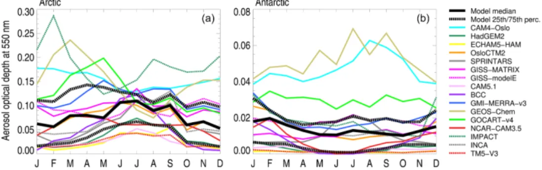
Figure 1. Mean seasonal cycle of the Arctic (60–90◦N) (a) and Antarctic (70–90◦S) (b) total AOD. The different colours represent the different AeroCom Phase II models. The black solid line is the model median and the dashed line is the 25th/75th percentile.
The AeroCom models ran simulations for the year 2006 (with emissions for the year 2000), while we compared AOD with observations from different available years in the period 2000–2015. Comparing 2006 AOD values from CALIOP (only available July–December) with the 2007–2012 aver-age, we find that 2006 is representative of the average (values varies 0–36 %).
3 Results
Here we present AOD and DAE results from the Arctic (de-fined as 60–90◦N) and the Antarctic (70–90◦S) regions. We compare the simulated seasonal AOD to ground-based measurements from a selection of stations in the Arctic and Antarctic. We also compare the modelled AOD with a re-trieval from MODIS over the Svalbard ocean region and with CALIOP. We then document the model-simulated regional patterns for each aerosol species.
3.1 Aerosol optical depth
Figure 1 shows the seasonal cycle of the total AOD in the Arctic and the Antarctic, for all the AeroCom Phase II mod-els. Values are for present-day conditions, i.e. emissions rep-resentative of the year 2000. The model-median AOD (Fig. 1, thick black line) has a summer maximum and a winter min-imum at both poles, but there is a large variation among the different models. For the Arctic, the spread is larger in winter and early spring and smaller during the summer months. A few models suggest an earlier Arctic AOD max-imum in winter (IMPACT) and early spring (GEOS-Chem and GOCART). For GEOS-Chem and GOCART this maxi-mum is dominated by natural aerosols (sea-salt and dust, re-spectively, as shown in Fig. 9). The higher values of AOD in CAM-Oslo are linked to efficient vertical transport in deep convective clouds, which exaggerates the amount of aerosols in the upper troposphere (and poleward transported aerosols). Note that modelled AOD is calculated from simu-lated aerosol distributions, and can therefore be reported even for months in which there is no actual sunlight.
3.1.1 Comparisons with measurements at both poles
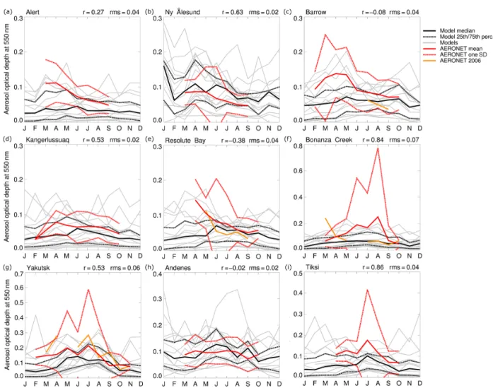
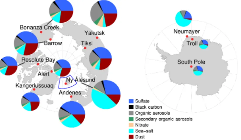
We have compared the seasonal cycle of modelled AOD with measurements from nine Arctic stations (details in Table 2), shown in Fig. 2. The AERONET mean (a climatology for all available years) is shown as a red line, and the model median is shown as a thick black line. The yellow line represents the year 2006, in which this was available. The AeroCom mod-els are shown as thin grey lines (for individual modmod-els, see Fig. S1 in the Supplement). The root mean square error and the correlation factor are shown for each site. We have calcu-lated the root mean square error (RMSE) as the square root of the average of the difference between the model median and AERONET values for each month. The values ranges from 0.02 (Ny-Ålesund, Kangerlussuaq, and Andenes) to 0.07 (Bonanza Creek). Alert, Ny-Ålesund, Barrow, and Res-olute Bay show the typical maximum in springtime AOD. Some models also show this peak, but the model median fails to capture the observed high spring AOD. The corre-lation factor for these stations is low (−0.08 to 0.27), except for Ny-Ålesund (0.63). Figure 3 shows the type of aerosol in terms of AOD that the models simulate for each station in spring (MAM) (JJA average in Fig. S2). Ny-Ålesund is dom-inated by sea-salt in spring, and the total AOD is larger than the other stations. There is a better agreement between mea-surements and models during the summer season when the observed AOD and its variability is lower. Bonanza Creek experienced unusually high August values in 2004, 2005, and 2009, resulting in a large SD. Here, the 2006 values for AERONET are closer to the model median in summer, but not in early spring. Tiksi station has the best correlation be-tween AERONET and the model median (0.86). This station has a maximum in AOD in summer, with large influences of organic aerosols from biomass burning (Fig. S2). Averaged over all nine stations, the annual mean AERONET AOD is 27 % higher compared to the model median AOD (excluding months without measurements). The correlation coefficient between the AeroCom and the AERONET monthly mean is 0.68 (P < 0.05). We would expect the spring peak in AOD to be stronger at the surface than for the total column. The
Figure 2. Seasonal cycle of model-median AOD compared to observations for nine Arctic stations: (a) Alert (82◦N, 62◦W), (b) Ny-Ålesund (78◦N, 11◦E), (c) Barrow (71◦N, 156◦W), (d) Kangerlussuaq (66◦N, 50◦W), (e) Resolute Bay (74◦N, 94◦W), (f) Bonanza Creek (64◦N, 148◦W), (g) Yakutsk (61◦N, 129◦E), (h) Andenes (69◦N, 16◦E), and (i) Tiksi (71◦N, 128◦E). The black solid line is the model median and the black dashed line is the 25th/75th percentile. Models are shown in thin, grey lines. The red solid line is the observational mean and the dashed red line is 1 SD from mean values. Measurements for (a–c) are taken Stone et al. (2014), (d–i) are from AERONET stations. Yellow lines are AOD measurements for the year 2006 (only available at a few stations).
age of Arctic air and its amplitude of the seasonal cycle with highest values in spring decrease strongly with altitude (Stohl, 2006), and the observed spring AOD is highest near the surface (Stone et al., 2010).
Figure 4 shows the spring (MAM) and summer (JJA) AOD for each model averaged over the nine Arctic stations, to-gether with the measured AERONET AOD. As is appar-ent from the correlation coefficiappar-ent (0.68) and the plots, the multi-model average is not a bad representation of the ob-served AOD, but the models vary altogether by a factor of 5–6 in magnitude. GOCART and GEOS-Chem are the mod-els closest to the observations in summer, and GMI-MERRA and IMPACT are the closest models in spring.
Retrievals of AOD from the MODIS satellite directly over snow and sea-ice are not available due to the high reflectiv-ity of these surfaces. Glantz et al. (2014) have provided spa-tial averages of MODIS AOD 555 nm over (darker) ocean
areas around Svalbard over a 9-year period (see Sect. 2). In our comparison, we have included this 9-year average to take into account the interannual spread in the data, even though the AeroCom models have simulated 1 year only. Figure 5a shows AOD over the Arctic Ocean (75–82◦N, 10◦W–40◦E) from MODIS retrieval 2003–2011 from Glantz et al. (2014) compared with the AeroCom models from April to Septem-ber. The retrieved AOD is approximately 0.1 in spring, but the uncertainty range is large: 0.115 ± 0.069 for MODIS and 0.093 ± 0.050 for AERONET (mean AOD ± 1 SD). The re-trieved AOD decreases over summer through to September. The AeroCom model mean also show a decrease throughout the year, but the slope is not as steep compared to MODIS. Some of the models shown in Fig. 5b) do have a steeper slope (GOCART, GISS-MATRIX, and GEOS-Chem). In the MODIS data the influence from large forest fire events and volcanic eruptions in summer has been removed to represent
Figure 3. The locations of the stations (red dots) with AOD measurements used in this study and the MODIS area (blue square). The circles show the modelled AOD species MAM average for each station. The area of the circles is scaled to the model median total AOD.
Figure 4. Multi-model AOD averaged for the spring (MAM) and summer (JJA) for the nine Arctic AERONET stations in Fig. 2 (details Table 2). The red bar is the average observation over the nine stations and the striped bar is the multi-model average. The error bars represent 1 SD.
background conditions, and this might be part of the reason why the models show higher values in summer compared to MODIS.
We have compared total AOD with the vertical integral of the monthly mean elastic backscatter at 532 nm from CALIOP. Figure 6 shows the seasonal cycle of AOD532 nm retrieval from CALIOP for the years 2006–2011 averaged over 60–82◦N compared to the AeroCom models screened by CALIOP availability (which is why June has zero num-bers north of 60◦N). The summer months are therefore dom-inated by biomass burning emissions at the southernmost lat-itudes. For all months except September, the model median lies within the range of the CALIOP retrievals. The corre-lation coefficient between the model median monthly mean and the CALIOP monthly mean is 0.75.
Figure 7 shows the measured seasonal cycle of AOD from three Antarctic stations (Neumayer, Troll, and the South Pole) compared to the AeroCom models. The Neumayer site is located closest to the ocean and has the highest
variabil-ity among the models. The correlation factor at Neumayer is 0.37, higher than at Troll (−0.26) and the South Pole (−0.04). Most models seem to be in the lower range of the observations. Tomasi et al. (2015) report multi-year sets of ground-based sun-photometer measurements conducted at nine Antarctic sites. For the high-altitude sites on the Antarc-tic Plateau (Dome Concordia 75◦S and South Pole 90◦S)
AOD is very stable, mainly ranging from 0.02 to 0.04. These values are slightly higher than the median AeroCom Phase II AOD (0.01).
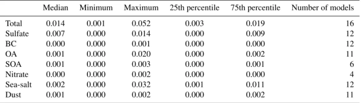
Figure 8 shows a box plot of the annual mean AOD in the Arctic and Antarctic for total aerosols and for the indi-vidual components (sulfate, BC from all sources, OA from all sources, SOA, nitrate, sea-salt, and dust). Model-median total AOD is 0.07 in the Arctic (with a model range of 0.02– 0.2), with the largest contribution to Arctic AOD from sul-fate (45 %). In the Antarctic the total AOD is 0.01 (0.001– 0.05) with sulfate being the largest model median compo-nent. However, sea-salt shows a large range with the 75th
Figure 5. AOD over the Arctic Ocean (75–82◦N, 10◦W–40◦E) from (a) MODIS retrieval 2003–2011 median (orange) compared to the AeroCom Phase II model mean (blue) and (b) the individual models. The error bars in (a) represent 1 SD.
Figure 6. AOD in the Arctic (60–82◦N) from CALIPSO retrieval for the different years 2006–2011 (AOD532 nm) (purple lines) com-pared to the AeroCom Phase II models (thin grey lines) screened by CALIOP availability.
percentile and the maximum value, which is much higher than the corresponding values for sulfate. Note that all mod-els have reported total AOD but not all the individual com-ponents’ AOD; see Table 1. The AOD median and 25th/75th percentiles values are listed in Tables 3 and 4.
Figure 9 shows the seasonal cycle of the AOD for the same individual components as in Fig. 8: sulfate, BC, OA, SOA, nitrate, sea-salt, and dust averaged over the Arctic re-gion (60–90◦N). There is a large spread between the mod-els. Most models show a peak in the AOD in summer, with a few models showing a late spring maximum. The geograph-ical distribution over the same region for the summer and winter season is shown in Fig. 10. For sulfate the highest model-mean AOD values in summer are found in the Rus-sian and northern Europe regions (0.09), while for BC the highest AOD values are found over Russia and eastern Asia (0.006). Both OAs and SOAs show a maximum in summer in the fire season with the highest AOD over Russia and eastern
Asia (0.07 and 0.02, respectively). Summer is also the season with maximum chemical production. In winter the AOD val-ues are low for OAs and SOAs. There is one outlier for OAs, CAM4-Oslo, which has very high marine primary OA emis-sions, and is the only model that includes MSA in the primary organics emissions (Tsigaridis et al., 2014). The emissions of aerosols (per mass) are dominated by sea-salt and dust. Since these emissions are mostly interactive (a function of wind speed and soil moisture for dust), a large model diversity in AOD is not surprising. Sea-salt AOD is highest during the winter season, with a maximum over the North Atlantic re-gion (0.1). The areas around the Norwegian Sea and Barents Sea have the highest cyclonic activity in winter (Serreze and Barrett, 2008). For dust aerosols, the models show a maxi-mum in spring/early summer and a secondary maximaxi-mum in September. The spring maximum originates most likely from dust storms in the Gobi and Taklamakan deserts, while the second smaller maximum in September might be due to local sources (Barrie and Barrie, 1990). GOCART shows higher AOD values for dust compared to the other models, proba-bly linked to an overestimation of dust emissions (Kim et al., 2014). Only four models have reported AOD from nitrate. The nitrate maximum is located over Eurasia in winter and over eastern Asia in summer.
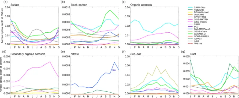
Figure 11 shows the seasonal cycle of AOD in the Antarc-tic for all the aerosol species. The model-median AOD has a maximum during the SH summer season of 0.02 and is reduced to about half during the winter season (0.01). Mod-elled BC, sulfate, and dust concentrations are highest during the winter months (SH summer). GISS-modelE shows higher values for SOAs. This model has the highest SOA lifetime (14 days) because of a large amount of SOAs in the upper troposphere, where there is less scavenging and more SOA available to be transported poleward. SPRINTARS shows the opposite behaviour on the seasonal cycle of sulfate AOD compared to the other models. This is likely linked to an anomaly in the relative humidity over East Antarctica in the
Figure 7. As Fig. 2, but for three Antarctic sites: Neumeyer 70◦S, 8◦W (a), Troll 72◦S, 2◦E (b), and South Pole 90◦S, 0◦E (c), with values from Tomasi et al. (2015).
Figure 8. Annual mean multi-model median AOD for the individual components (sulfate, BC (from all sources), total OA (from all sources), SOA, nitrate, sea-salt, and dust) and the total aerosol, averaged over the Arctic (60–90◦N) (a) and the Antarctic (70–90◦S) (b). The bottom and top of each box are the first and third (25th/75th) quartiles, and the band inside the box is the model median. The whiskers represent the minimum and maximum of the model range. Note the different vertical axis – the right-hand vertical axis is for total AOD.
Figure 9. Seasonal cycle multi-model Arctic AOD for (a) sulfate, (b) BC (from all sources), (c) total OA (from all sources), (d) SOA, (e) nitrate, (f) sea-salt, and (g) dust. The Arctic region is defined as 60–90◦N. Note the different axes.
Table 3. Annual mean Arctic (60–90◦N) AOD AeroCom Phase II model median, model range (minimum and maximum), and the 25th/75th percentile. The number of models for each species is given in the rightmost column. BC is total BC from all sources and OA is total OA from all sources.
Median Minimum Maximum 25th percentile 75th percentile Number of models
Total 0.071 0.025 0.183 0.031 0.121 16 Sulfate 0.032 0.003 0.068 0.009 0.044 12 BC 0.002 0.000 0.004 0.001 0.003 12 OA 0.014 0.001 0.072 0.006 0.017 11 SOA 0.004 0.001 0.012 0.002 0.007 6 Nitrate 0.001 0.000 0.011 0.000 0.003 4 Sea-salt 0.013 0.001 0.054 0.007 0.018 12 Dust 0.008 0.001 0.035 0.003 0.014 11
Table 4. As Table 3, but averaged over the Antarctic region (70–90◦S).
Median Minimum Maximum 25th percentile 75th percentile Number of models
Total 0.014 0.001 0.052 0.003 0.019 16 Sulfate 0.007 0.000 0.014 0.000 0.009 12 BC 0.000 0.000 0.001 0.000 0.000 12 OA 0.001 0.000 0.020 0.000 0.002 11 SOA 0.001 0.000 0.003 0.000 0.001 6 Nitrate 0.000 0.000 0.002 0.000 0.000 4 Sea-salt 0.002 0.000 0.032 0.001 0.011 12 Dust 0.001 0.000 0.002 0.000 0.002 11
Table 5. Annual mean Arctic (60–90◦N) DAE AeroCom Phase II model median, model range (minimum and maximum), and the 25th/75th percentile. The number of models for each species is given in the rightmost column. BC FF is BC from fossil fuel and biofuel emissions and OA FF is OA from fossil fuel and biofuel emissions. BB is BC and AO combined from biomass burning emissions.
Median Minimum Maximum 25th percentile 75th percentile Number of models
Total −0.12 −0.30 0.09 −0.22 0.01 16 Sulfate −0.24 −0.43 0.01 −0.29 −0.11 14 BC FF 0.19 0.03 0.37 0.12 0.26 14 OA FF 0.00 −0.04 0.02 −0.02 0.00 14 BB 0.01 −0.06 0.04 −0.02 0.02 13 SOA −0.01 −0.12 0.01 −0.02 0.00 5 Nitrate −0.03 −0.09 0.00 −0.06 −0.01 6
simulation and has been improved in a newer version of the model. The high sea-salt values in Geos-Chem have been linked to an overestimation of sea-salt under high-wind con-ditions at middle and high latitudes (Jaeglé et al., 2011). By adding a SST-dependent source function, the model bias was reduced from +64 to +33 % for cruise measurements and from +32 to −5 % for ground-based sites. GMI-MERRA shows higher nitrate AOD values compared to the other models and is probably linked to the inclusion of oceanic NH3 emissions (based on the GEIA emission inventory) in
the model. The CMIP5 emission data set does not include NH3 oceanic emissions. For a first assessment of nitrate
from multiple models compared with observations, see Bian et al. (2017). Nine models from the AeroCom Phase III
trate experiment show large diversity in their simulated ni-trate concentrations, especially in remote regions. The au-thors link this spread to the involvement of nitrate in compli-cated chemistry and the concentrations of nitrate depending on accurate simulations of precursors (NH3, HNO3, dust, and
sea-salt).
3.2 Aerosol direct radiative forcing
The DAE is calculated as the difference between the reflected solar radiation at TOA between simulations with present-day (2000) and pre-industrial (1850) emissions of anthropogenic aerosols and precursors. Figure 12 shows the multi-model DAE for sulfate, BC FF (from fossil fuel and biofuel
emis-Table 6. As emis-Table 5, but averaged over the Antarctic region (70–90◦S).
Median Minimum Maximum 25th percentile 75th percentile Number of models
Total 0.03 0.00 0.10 0.01 0.07 16 Sulfate 0.00 −0.03 0.00 −0.01 0.00 14 BC FF 0.02 0.00 0.09 0.01 0.04 14 OA FF 0.00 0.00 0.01 0.00 0.00 14 BB 0.01 −0.01 0.08 0.00 0.02 13 SOA 0.00 0.00 0.01 0.00 0.00 5 Nitrate 0.00 0.00 0.03 0.00 0.00 6
Figure 10. The geographical distributed model-median Arctic AOD (a) sulfate, (b) BC (from all sources), (c) total OA (from all sources), (d) SOA, (e) nitrate, (f) sea-salt, and (g) dust, for the summer (JJA) season (left) and the winter (DJF) season (right). Note the different axes.
sions), OA FF (from fossil fuel and biofuel emissions), BB, SOA, nitrate, and the total, averaged in the Arctic and the Antarctic regions. In the Arctic, the dominant aerosol forc-ing agents are BC FF and sulfate with model-median DAE estimated at +0.19 and −0.24 W m−2, respectively, although
the Arctic AOD of BC is low compared to the other aerosols (Fig. 8). The other treated species are relatively low both in burden and in modelled DAE. The Arctic annual mean multi-model-median DAE is −0.12 W m−2 (with the 25th, 75th percentile; −0.22, 0.01). The Antarctic model-median DAE
Figure 11. Multi-model seasonal cycle Antarctic mean (70–90◦S) AOD for the individual components (a) sulfate, (b) BC (from all sources), (c) total OA (from all sources), (d) SOA, (e) nitrate, (f) sea-salt, and (g) dust. Note the different axes.
Figure 12. Annual mean multi-model DAE (in W m−2) averaged over the Arctic (60–90◦N) (a) and the Antarctic (70–90◦S) (b) for the individual components (sulfate, BC FF, OA FF, BB, SOA, and nitrate) and the total aerosol. The bottom and top of each box are the first and third (25th/75th) quartiles, and the band inside the box is the model median. The whiskers represent the minimum and maximum of the model range. Note the different vertical axis.
is 0.03 W m−2(0.01, 0.07). The two largest forcing compo-nents here are BC FF and BB. Note that only the direct ra-diative forcing is reported. The numbers are listed in Tables 5 and 6.
Figure 13 shows the Arctic DAE seasonal cycle. The di-rect influence of aerosols on the radiation budget in the Arc-tic shifts from a BC-driven positive DAE during the spring months, to a sulfate-driven negative forcing in late summer, caused by higher surface albedo from sea-ice and snow in the former season (Ødemark et al., 2012). Also shown in Fig. 13 is the geographical distribution of DAE in summer (JJA), and a balance between sulfate and BC FF is also apparent here linked to albedo. Negative DAE from sulfate dominates land areas outside the high Arctic, while higher positive DAE from BC FF is evident in the high Arctic and in the Pacific.
Even though the AOD of BC is low in the Arctic, the DAE from BC FF dominates the total DAE in spring. In Fig. 14 we
have normalized the JJA DAE (for total, sulfate, and BC FF) to AOD (total, sulfate and BC) to illustrate this. The total normalized forcing is positive in the high Arctic due to the high efficiency of the BC forcing. Outside the high Arctic, there is a band of negative direct forcing due to sulfate. 3.3 Sensitivity simulations with GISS modelE
The model-spread for aerosols at the poles is large and not entirely surprising, given the large sensitivity to remote trans-port for aerosol concentrations at high latitudes. The rea-sons for this spread include transport and removal mecha-nisms and the interaction between them. To illustrate some of the variation we have performed sensitivity tests with one of the AeroCom models, GISS modelE. The anthropogenic BC emissions (from fossil fuel and biofuel) have been dou-bled in southern Asia, eastern Asia, and Russia, and Fig. 18a shows the resulting (total) BC AOD in the Arctic for the
Figure 13. Arctic mean DAE seasonal cycle and the summer (JJA) mean model-media n geographical distribution of (a) total aerosol, (b) sulfate, (c) BC FF, (d) OA FF, (e) BB, (f) SOA, and (g) nitrate. Note the different axes.
(a) Total (b) Sulfate (c) Black carbon
Figure 14. JJA mean model-median normalized DAE, i.e. total DAE (in W m−2) per total AOD (a), sulfate DAE per sulfate AOD (b), and BC FF DAE per BC AOD (c). Note the different axes.
Figure 15. Arctic annual mean DAE (in W m−2) for the AeroCom Phase II models, total (a), sulfate (b), BC FF (c). The striped bar is the model mean. TM5-V3 and CM4-Oslo have reported the total only.
Figure 16. Arctic annual mean DAE per AOD for all AeroCom Phase II models, total (a), sulfate (b), and BC FF (c). Values for sulfate and BC are missing for GEOS-Chem, IMPACT, NCAR-CAM3.5, GISS-MATRIX, CAM4-Oslo and TM5 (see Table 1).
different regional emission perturbations. The annual mean BC AOD in the Arctic increases by 33 % from a doubling of the BC FF emissions in East Asia, while doubling in south-ern Asia and Russia increase the BC AOD by 10 and 8 %, respectively. The change in AOD from a doubling in emis-sions is still within the AeroCom model range, shown in grey lines. Here we only show plots for the Arctic, but the increase in BC AOD in Antarctica is not negligible: 28 % increase for a doubling in eastern Asia and 7 % for a dou-bling in southern Asia (zero for Russia) (Fig. S2). We have also tested the sensitivity to the e-folding time of BC from hydrophobic (fresh) to hydrophilic (aged) state. GISS mod-elE has a BC global lifetime of 5.9 days, which is close to the AeroCom average global lifetime of 6.5 days (it ranges from 3.8 days in CAM5.1 to 17.1 days in HadGEM2) (Sam-set et al., 2014). Figure 18b shows the resulting change in BC AOD in Arctic by (1) doubling the e-folding time and (2) reducing it by 50 %. By reducing the e-folding time by half, BC decreases by 30 % at both poles. However, by making the lifetime longer by doubling the e-folding time, the BC AOD
increases with 36–39 % at both poles. The change in BC is still within the AeroCom model range.
Figure 15 shows the multi-model DAE in the Arc-tic, sorted by highest-to-lowest, for total aerosol and for sulfate and BC FF. Most models have an annual mean negative net DAE in the Arctic, ranging from −0.3 to 0.0 W m−2, while five models show a positive net DAE (CAM4-Oslo, HadGEM2, OsloCTM2, GEOS-Chem, and CAM5.1). These latter models have a lower-than-average negative sulfate forcing (HadGEM2, CAM5.1, OsloCTM2), and/or higher-than-average positive BC FF forcing (GEOS-Chem, OsloCTM2, and HadGEM2). When normalizing the Arctic DAE with AOD for each model (Fig. 16), it is ap-parent that some models have a high forcing efficiency for sulfate (HAM2) and/or BC FF (BCC, ECHAM5-HAM2).
Figure 17 shows the seasonal cycle of DAE for total aerosols and for sulfate, BC FF, OA FF, BB, SOA, and ni-trate in Antarctica. There is a large spread in DAE during SH summer season, with values ranging from 0 to 0.3 W m−2, dominated by BC DAE. Several of the models that have the
Figure 17. Antarctic mean (70–90◦S) seasonal cycle of (a) the total DAE and the DAE for (b) sulfate, (c) BC FF, (d) OA FF, (e) BB, (f) SOA, and (g) nitrate. Note the different axes.
Figure 18. Arctic mean seasonal cycle of (total) BC AOD for simulations with GISS modelE (in colours) compared to the AeroCom models (in light grey). Panel (a) shows the experiment with doubling the emissions, while panel (b) shows the effect of changing the e-folding lifetime. The darker grey AeroCom model is the GISS modelE AeroCom run. Panel (a) shows emission perturbations for a doubling of BC emissions (fossil fuel and biofuel) in southern Asia (green), eastern Asia (red), Russia (yellow), and global (blue). Panel (b) shows double (red) and half (green) of the e-folding time from hydrophobic to hydrophilic BC.
highest (positive) BC FF DAE also have the highest (nega-tive) sulfate DAE, as indicated by Myhre et al. (2013). As these models do not show particularly strong forcing per unit AOD (see e.g. Fig. 16), but generally have high values for Antarctic AOD (Fig. 11), we attribute this correlation to effi-cient transport of aerosols to the South Pole region.
4 Summary and discussion
We have reported on modelled AOD and DAE at both poles, and compared individual and multi-model results to
avail-able measurements. Defining the Arctic as the 60–90◦N re-gion, the dominant aerosol species, in terms of AOD, are sul-fate, sea-salt, and OA. The total model-median AOD is 0.07, which is close to observed AOD. However, the intermodel spread is very wide (0.02–0.18). Compared to measurements at nine Arctic stations, most models tend to underestimate the AOD, especially the build-up of aerosols in early winter and spring. Seasonally, the influence of aerosols on the Arctic energy balance shifts from a BC-driven positive DAE during the spring months, to a sulfate-driven negative DAE in late summer. Despite a relatively low Arctic BC AOD compared
to the other aerosols, the BC FF DAE dominates in spring with an annual mean model median of 0.19 W m−2 (0.12, 0.26 W m−225th/75th percentiles). The total Arctic annual mean DAE model median is slightly negative, −0.12 W m−2 (−0.22, 0.01). We note, however, that this estimate of Arctic aerosol radiative forcing does not include semi- or indirect cloud effects, or surface albedo modification. The Arctic sur-face radiative forcing from BC in snow has been estimated at 0.18 W m−2using deposited fields from the AeroCom Phase II models into an offline land and sea-ice model (Jiao et al., 2014). There are few estimates of the semi-direct effects of aerosols, which is mostly due to BC. Bond et al. (2013) in-dicates a −0.1 W m−2global effect, equally split between di-rect and indidi-rect effects, while a later study also indicates that the semi-direct effect counteracts about 50 % of the direct effect, independent of altitude (Samset and Myhre, 2015). None of these estimates are made specifically for the Arctic. Indirect cloud effects are likely different in the Arctic than at lower latitudes, in large part because of the already bright surfaces in the Arctic. Also, cloud emissivity might be more important here, as thermal radiation dominates the dark win-ter months (Garrett et al., 2004).
The models also predict a fair amount of aerosol trans-port to the Antarctic region (defined here as 70–90◦S). In Antarctica, modelled AOD is smaller in magnitude than in the Arctic, with an annual mean of 0.01 (0.001–0.05 model range). Compared to limited available measurements, these values might be on the lower end of the spectrum. As in the Arctic, the dominant aerosol species is sulfate. The dominant aerosol forcing agent in the Antarctic, however, is BC, result-ing in a small, but positive DAE in this region (0.03 W m−2). Again, this does not include possible additional effects of sur-face albedo modification (Jiao et al., 2014).
Not surprisingly, the spread in modelled AOD at both poles is large. The relative spread in DAE is larger than the relative spread in AOD, linked to each model’s radiation pa-rameterization (Stier et al., 2013). Sensitivity experiments of BC with one of the AeroCom models reveal that the Arctic BC AOD is sensitive to the emissions and lifetime of BC. A doubling of fossil fuel and biofuel emissions in eastern Asia results in a 33 % increase in Arctic BC AOD. How-ever, radical changes such as reducing the e-folding lifetime by half or doubling it, still fall within the AeroCom model range.
The AeroCom data are only available as monthly aver-ages, and we have therefore compared them with monthly averaged retrievals from AERONET and CALIOP/MODIS. Schutgens et al. (2016a, b) suggests that models should be temporally collocated to the observations before comparing the data to prevent sampling errors. In their study three global models were compared to AERONET/MODIS and sampling errors up to 100 % in AOD were apparent for yearly and monthly averages. Since the AeroCom data are only provided monthly, this is a potential problem both for this and most other AeroCom studies.
Various factors lie behind the large spread in modelled AOD in the polar regions. Recommendations to improve our understanding of the role of aerosols in the polar regions and to reduce the uncertainties include sensitivity tests on removal processes (Wang et al., 2013; Liu et al., 2011; Bour-geois and Bey, 2011) and resolution (Ma et al., 2014) dur-ing transport to the Arctic, up to date treatment of aerosol mixtures and missing emission sources (Stohl et al., 2013; Evangeliou et al., 2016), and a better characterization of mea-surement uncertainties in satellite data over polar land and oceans. Of these, updated emission inventories (global and polar) and model validation of AODs and column loadings against local observations seem most crucial for providing a solid baseline for evaluations of transport schemes and cal-culations of radiative forcing, taking into account a broader range of physical effects.
Data availability. AeroCom data and CALIOP data are available through http://aerocom.met.no. Sensitivity studies and further anal-ysis results are available upon request to Maria Sand. AERONET data are available at http://aeronet.gsfc.nasa.gov/.
The Supplement related to this article is available online at https://doi.org/10.5194/acp-17-12197-2017-supplement.
Acknowledgements. Maria Sand has received funding from The Research Council of Norway (RCN) through a FRIPRO Mobility Grant, BlackArc, contract no 240921. The FRIPRO Mobility grant scheme (FRICON) is co-funded by the European Union’s Seventh Framework Programme for research, technological devel-opment and demonstration under Marie Curie grant agreement no 608695. Maria Sand and Bjørn H. Samset were funded through the Polish-Norwegian Research Programme project iAREA, and RCN projects AEROCOM-P3 and AC/BC (240372). Richard C. Easter and Steven J. Ghan were supported by the US Department of Energy Office of Science Decadal and Regional Climate Prediction using Earth System Models (EaSM) programme. The Pacific Northwest National Laboratory is operated for the DOE by Battelle Memorial Institute under contract DE-AC06-76RLO 1830. Guangxing Lin and Joyce E. Penner were supported by the National Science Foundation (projects AGS-0946739 and ARC-1023387) and the Department of Energy (DOE FG02 01 ER63248 and DOE DE-SC0008486. Toshihiko Takemura is supported by the NEC SX-ACE supercomputer system of the National Institute for Environmental Studies, Japan, the Environmental Research and Technology Development Fund (S-12-3) of the Ministry of Envi-ronment, Japan and JSPS KAKENHI Grant Numbers JP15H01728 and JP15K12190. Trond Iversen, Alf Kirkevåg and Øyvind Seland were supported by the Norwegian Research Council through the projects EVA (grant 229771), EarthClim (207711/E10), NOTUR (nn2345k), and NorStore (ns2345k), and through the EU projects PEGASOS and ACCESS and Nordforsk-CRAICC. Philip Stier acknowledges funding from the European Research Council (ERC) under the European Union’s Seventh Framework Programme
(FP7/2007–2013) ERC project ACCLAIM (Grant Agreement FP7-280025) and from the UK Natural Environment Research Council project GASSP (grant number NE/J022624/1). The CESM project is supported by the National Science Foundation and the Office of Science (BER) of the US Department of Energy. NCAR is sponsored by the National Science Foundation. CALIPSO is a joint satellite mission between NASA and the French Agency, CNES. Guangxing Lin and Fangqun Yu were supported by the National Aeronautics and Space Administration (NASA NNX17AG35G) and the National Science Foundation (NSF AGS-1550816). We thank the PI investigators and their staff for establishing and maintaining the AERONET sites used in this study. Edited by: Maria Kanakidou
Reviewed by: two anonymous referees
References
Albrecht, B. A.: Aerosols, cloud microphysics, and fractional cloudiness, Science, 245, 1227–1230, 1989.
AMAP: The Impact of Black Carbon on Arctic Climate, Arctic Monitoring and Assessment Programme (AMAP), Oslo, Nor-way, p. 70, 2011.
Arimoto, R., Hogan, A., Grube, P., Davis, D., Webb, J., Schloesslin, C., Sage, S., and Raccah, F.: Major ions and radionuclides in aerosol particles from the South Pole during ISCAT-2000, Atmos. Environ., 38, 5473–5484, https://doi.org/10.1016/j.atmosenv.2004.01.049, 2004.
Barrie, L. A. and Barrie, M. J.: Chemical components of lower tro-pospheric aerosols in the high Arctic: Six years of observation, J. Atmos. Chem., 11, 211–226, 1990.
Bauer, S. E., Wright, D. L., Koch, D., Lewis, E. R., McGraw, R., Chang, L.-S., Schwartz, S. E., and Ruedy, R.: MATRIX (Mul-ticonfiguration Aerosol TRacker of mIXing state): an aerosol microphysical module for global atmospheric models, Atmos. Chem. Phys., 8, 6003–6035, https://doi.org/10.5194/acp-8-6003-2008, 2008.
Bellouin, N., Rae, J., Jones, A., Johnson, C., Haywood, J., and Boucher, O.: Aerosol forcing in the Climate Model Intercom-parison Project (CMIP5) simulations by HadGEM2-ES and the role of ammonium nitrate, J. Geophys. Res., 116, D20206, https://doi.org/10.1029/2011JD016074, 2011.
Bian, H., Chin, M., Rodriguez, J. M., Yu, H., Penner, J. E., and Strahan, S.: Sensitivity of aerosol optical thickness and aerosol direct radiative effect to relative humidity, Atmos. Chem. Phys., 9, 2375–2386, https://doi.org/10.5194/acp-9-2375-2009, 2009. Bian, H., Chin, M., Hauglustaine, D. A., Schulz, M., Myhre, G.,
Bauer, S. E., Lund, M. T., Karydis, V. A., Kucsera, T. L., Pan, X., Pozzer, A., Skeie, R. B., Steenrod, S. D., Sudo, K., Tsigaridis, K., Tsimpidi, A. P., and Tsyro, S. G.: Investigation of global nitrate from the AeroCom Phase III experiment, Atmos. Chem. Phys. Discuss., https://doi.org/10.5194/acp-2017-359, in review, 2017. Bigg, E. K.: Comparison of Aerosol at Four Base-line Atmospheric Monitoring Stations, J. Appl. Me-teorol., 19, 521–533, https://doi.org/10.1175/1520-0450(1980)019<0521:COAAFB>2.0.CO;2, 1980.
Bond, T. C., Doherty, S. J., Fahey, D. W., Forster, P. M., Berntsen, T., DeAngelo, B. J., Flanner, M. G., Ghan, S.,
Kärcher, B., Koch, D., Kinne, S., Kondo, Y., Quinn, P. K., Sarofim, M. C., Schultz, M. G., Schulz, M., Venkatara-man, C., Zhang, H., Zhang, S., Bellouin, N., Guttikunda, S. K., Hopke, P. K., Jacobson, M. Z., Kaiser, J. W., Klimont, Z., Lohmann, U., Schwarz, J. P., Shindell, D., Storelvmo, T., War-ren, S. G., and Zender, C. S.: Bounding the role of black carbon in the climate system: A scientific assessment, J. Geophys. Res.-Atmos., 18, 5380–5552, https://doi.org/10.1002/jgrd.50171, 2013.
Boucher, O., Randall, D., Artaxo, P., Bretherton, C., Feingold, G., Forster, P., Kerminen, V.-M., Kondo, Y., Liao, H., Lohmann, U., Rasch, P., Satheesh, S. K., Sherwood, S., Stevens, B., and Zhang, X. Y.: Clouds and aerosols, in: Climate Change 2013: The Physical Science Basis. Contribution of Working Group I to the Fifth Assessment Report of the Intergovernmental Panel on Climate Change, edited by: Stocker, T. F., Qin, D., Plattner, G.-K., Tignor, M., Allen, S. G.-K., Boschung, J., Nauels, A., Xia, Y., Bex, V., and Midgley, P. M., Cambridge University Press, Cam-bridge, UK and New York, NY, USA, pp. 571–657, 2013. Bourgeois, Q. and Bey, I.: Pollution transport efficiency
toward the Arctic: Sensitivity to aerosol scavenging and source regions, J. Geophys. Res., 116, D08213, https://doi.org/10.1029/2010JD015096, 2011.
Browse, J., Carslaw, K. S., Mann, G. W., Birch, C. E., Arnold, S. R., and Leck, C.: The complex response of Arctic aerosol to sea-ice retreat, Atmos. Chem. Phys., 14, 7543–7557, https://doi.org/10.5194/acp-14-7543-2014, 2014.
Clarke, A. D. and Noone, K. J.: Soot in the Arctic snowpack: a cause for perturbations in radiative transfer, Atmos. Environ., 19, 2045–2053, https://doi.org/10.1016/0004-6981(85)90113-1, 1985.
Eckhardt, S., Quennehen, B., Olivié, D. J. L., Berntsen, T. K., Cherian, R., Christensen, J. H., Collins, W., Crepinsek, S., Daskalakis, N., Flanner, M., Herber, A., Heyes, C., Hodnebrog, Ø., Huang, L., Kanakidou, M., Klimont, Z., Langner, J., Law, K. S., Lund, M. T., Mahmood, R., Massling, A., Myriokefali-takis, S., Nielsen, I. E., Nøjgaard, J. K., Quaas, J., Quinn, P. K., Raut, J.-C., Rumbold, S. T., Schulz, M., Sharma, S., Skeie, R. B., Skov, H., Uttal, T., von Salzen, K., and Stohl, A.: Current model capabilities for simulating black carbon and sulfate concentra-tions in the Arctic atmosphere: a multi-model evaluation using a comprehensive measurement data set, Atmos. Chem. Phys., 15, 9413–9433, https://doi.org/10.5194/acp-15-9413-2015, 2015. Evangeliou, N., Balkanski, Y., Hao, W. M., Petkov, A., Silverstein,
R. P., Corley, R., Nordgren, B. L., Urbanski, S. P., Eckhardt, S., Stohl, A., Tunved, P., Crepinsek, S., Jefferson, A., Sharma, S., Nøjgaard, J. K., and Skov, H.: Wildfires in northern Eurasia af-fect the budget of black carbon in the Arctic – a 12-year retro-spective synopsis (2002–2013), Atmos. Chem. Phys., 16, 7587– 7604, https://doi.org/10.5194/acp-16-7587-2016, 2016. Fiebig, M., Lunder, C. R., and Stohl, A.: Tracing biomass
burning aerosol from South America to Troll Research Station, Antarctica, Geophys. Res. Lett., 36, L14815, https://doi.org/10.1029/2009GL038531, 2009.
Flanner, M. G., Zender, C. S., Hess, P. G., Mahowald, N. M., Painter, T. H., Ramanathan, V., and Rasch, P. J.: Springtime warming and reduced snow cover from carbonaceous particles, Atmos. Chem. Phys., 9, 2481–2497, https://doi.org/10.5194/acp-9-2481-2009, 2009.
Garrett, T. J, Zhao, C., Dong, X., Mace, G. G., and Hobbs, P. V.: Effects of varying aerosol regimes on low-level Arctic stratus, Geophys. Res. Lett., 31, L17105, https://doi.org/10.1029/2004GL019928, 2004.
Glantz, P., Bourassa, A., Herber, A., Iversen, T., Karls-son, J., Kirkevåg, A., Maturilli, M., Seland, Ø., Stebel, K., Struthers, H., Tesche, M., and Thomason, L.: Remote sens-ing of aerosols in the Arctic for an evaluation of global cli-mate model simulations, J. Geophys. Res., 119, 8169–8188, https://doi.org/10.1002/2013JD021279, 2014.
Hansen, J. and Nazarenko, L.: Soot climate forcing via snow and ice albedos, P. Natl. Acad. Sci. USA, 101, 423–428, https://doi.org/10.1073/pnas.2237157100, 2004.
Hansen, J., Sato, M., and Ruedy, R.: Radiative forcing and climate response, J. Geophys. Res.-Atmos., 102, 6831–6864, https://doi.org/10.1029/96JD03436, 1997.
Hara, K., Osada, K., Kido, M., Hayashi, M., Matsunaga, K., Iwasaka, Y., Yamanouchi, T., Hashida, G., and Fukatsu, T.: Chemistry of sea-salt particles and inorganic halogen species in Antarctic regions: Compositional differences between coastal and inland stations, J. Geophys. Res., 109, D20208, https://doi.org/10.1029/2004JD004713, 2004.
von Hardenberg, J., Vozella, L., Tomasi, C., Vitale, V., Lupi, A., Mazzola, M., van Noije, T. P. C., Strunk, A., and Proven-zale, A.: Aerosol optical depth over the Arctic: a compar-ison of ECHAM-HAM and TM5 with ground-based, satel-lite and reanalysis data, Atmos. Chem. Phys., 12, 6953–6967, https://doi.org/10.5194/acp-12-6953-2012, 2012.
Hartmann, D., Klein Tank, A., Rusticucci, M., Alexander, L., Broennimann, B., Charabi, Y., Dentener, F., Dlugokencky, E., Easterling, D., Kaplan, A., Soden, B., Thorne, P., Wild, M., and Zhai, P.: Observations: atmosphere and surface, in: Cli-mate Change 2013: The Physical Science Basis. Contribution of Working Group I to the Fifth Assessment Report of the Intergov-ernmental Panel on Climate Change, edited by: Stocker, T. F., Qin, D., Plattner, G.-K., Tignor, M., Allen, S. K., Boschung, J., Nauels, A., Xia, Y., Bex, V., and Midgley, P. M., Cambridge Uni-versity Press, Cambridge, UK and New York, NY, USA, 2013. Haywood, J. M. and Shine, K. P.: The effect of
anthro-pogenic sulfate and soot aerosol on the clear sky plan-etary radiation budget, Geophys. Res. Lett., 22, 603–606, https://doi.org/10.1029/95GL00075, 1995.
Hirdman, D., Sodemann, H., Eckhardt, S., Burkhart, J. F., Jeffer-son, A., Mefford, T., Quinn, P. K., Sharma, S., Ström, J., and Stohl, A.: Source identification of short-lived air pollutants in the Arctic using statistical analysis of measurement data and par-ticle dispersion model output, Atmos. Chem. Phys., 10, 669–693, https://doi.org/10.5194/acp-10-669-2010, 2010.
Hodnebrog, Ø., Myhre, G., and Samset, B. H.: How shorter black carbon lifetime alters its climate effect, Nat. Commun., 5, 5065, https://doi.org/10.1038/ncomms6065, 2014.
Holben, B. N., Eck, T. F., Slutsker, I., Tanré, D., Buis, J. P., Setzer, A., Vermote, E., Reagan, J. A., Kaufman, Y. J., Nakajima, T., Lavenu, F., Jankowiak, I., and Smirnov, A.: AERONET – a federated instrument network and data archive for aerosol characterization, Remote Sens. Environ., 66, 1–16, https://doi.org/10.1016/S0034-4257(98)00031-5, 1998.
Iversen, T. and Joranger, E.: Arctic air pollution and large scale atmospheric flows, Atmos. Environ., 19, 2099–2108, https://doi.org/10.1016/0004-6981(85)90117-9, 1985.
Jaeglé, L., Quinn, P. K., Bates, T. S., Alexander, B., and Lin, J.-T.: Global distribution of sea salt aerosols: new constraints from in situ and remote sensing observations, Atmos. Chem. Phys., 11, 3137–3157, https://doi.org/10.5194/acp-11-3137-2011, 2011. Jiao, C., Flanner, M. G., Balkanski, Y., Bauer, S. E., Bellouin, N.,
Berntsen, T. K., Bian, H., Carslaw, K. S., Chin, M., De Luca, N., Diehl, T., Ghan, S. J., Iversen, T., Kirkevåg, A., Koch, D., Liu, X., Mann, G. W., Penner, J. E., Pitari, G., Schulz, M., Se-land, Ø., Skeie, R. B., Steenrod, S. D., Stier, P., Takemura, T., Tsigaridis, K., van Noije, T., Yun, Y., and Zhang, K.: An Aero-Com assessment of black carbon in Arctic snow and sea ice, At-mos. Chem. Phys., 14, 2399–2417, https://doi.org/10.5194/acp-14-2399-2014, 2014.
Kim, D., Chin, M., Yu, H., Diehl, T., Tan, Q., Kahn, R. A., Tsigaridis, K., Bauer, S. E., Takemura, T., Pozzoli, L., Bel-louin, N., Schulz, M., Peyridieu, S., Chédin, A., and Koffi, B.: Sources, sinks, and transatlantic transport of North African dust aerosol: A multimodel analysis and comparison with remote sensing data, J. Geophys. Res., 119, 6259–6277, https://doi.org/10.1002/2013JD021099, 2014.
Kipling, Z., Stier, P., Johnson, C. E., Mann, G. W., Bellouin, N., Bauer, S. E., Bergman, T., Chin, M., Diehl, T., Ghan, S. J., Iversen, T., Kirkevåg, A., Kokkola, H., Liu, X., Luo, G., van Noije, T., Pringle, K. J., von Salzen, K., Schulz, M., Seland, Ø., Skeie, R. B., Takemura, T., Tsigaridis, K., and Zhang, K.: What controls the vertical distribution of aerosol? Relationships be-tween process sensitivity in HadGEM3–UKCA and inter-model variation from AeroCom Phase II, Atmos. Chem. Phys., 16, 2221–2241, https://doi.org/10.5194/acp-16-2221-2016, 2016. Kirkevåg, A., Iversen, T., Seland, Ø., Hoose, C., Kristjánsson,
J. E., Struthers, H., Ekman, A. M. L., Ghan, S., Griesfeller, J., Nilsson, E. D., and Schulz, M.: Aerosol–climate interac-tions in the Norwegian Earth System Model – NorESM1-M, Geosci. Model Dev., 6, 207–244, https://doi.org/10.5194/gmd-6-207-2013, 2013.
Koch, D. and Hansen, J.: Distant origins of Arctic black carbon: A Goddard Institute for Space Studies ModelE experiment, J. Geophys. Res., 110, D04204, https://doi.org/10.1029/2004JD005296, 2005.
Koch, D., Schulz, M., Kinne, S., McNaughton, C., Spackman, J. R., Balkanski, Y., Bauer, S., Berntsen, T., Bond, T. C., Boucher, O., Chin, M., Clarke, A., De Luca, N., Dentener, F., Diehl, T., Dubovik, O., Easter, R., Fahey, D. W., Feichter, J., Fillmore, D., Freitag, S., Ghan, S., Ginoux, P., Gong, S., Horowitz, L., Iversen, T., Kirkevåg, A., Klimont, Z., Kondo, Y., Krol, M., Liu, X., Miller, R., Montanaro, V., Moteki, N., Myhre, G., Penner, J. E., Perlwitz, J., Pitari, G., Reddy, S., Sahu, L., Sakamoto, H., Schuster, G., Schwarz, J. P., Seland, Ø., Stier, P., Takegawa, N., Takemura, T., Textor, C., van Aardenne, J. A., and Zhao, Y.: Eval-uation of black carbon estimations in global aerosol models, At-mos. Chem. Phys., 9, 9001–9026, https://doi.org/10.5194/acp-9-9001-2009, 2009.
Koch, D., Bauer, S. E., Del Genio, A., Faluvegi, G., Mc-Connell, J. R., Menon, S., Miller, R. L., Rind, D., Ruedy, R., Schmidt, G. A., and Shindell, D.: Coupled aerosol-chemistry– climate twentieth-century transient model investigation: trends in