A geostatistical approach to multisensor rain field reconstruction and downscaling

HAL Id: hal-00304595

https://hal.archives-ouvertes.fr/hal-00304595

Submitted on 1 Jan 2001

HAL is a multi-disciplinary open access archive for the deposit and dissemination of sci-entific research documents, whether they are pub-lished or not. The documents may come from teaching and research institutions in France or abroad, or from public or private research centers.

L’archive ouverte pluridisciplinaire HAL, est destinée au dépôt et à la diffusion de documents scientifiques de niveau recherche, publiés ou non, émanant des établissements d’enseignement et de recherche français ou étrangers, des laboratoires publics ou privés.

reconstruction and downscaling

P. Fiorucci, P. La Barbera, L.G. Lanza, R. Minciardi

To cite this version:

P. Fiorucci, P. La Barbera, L.G. Lanza, R. Minciardi. A geostatistical approach to multisensor rain field reconstruction and downscaling. Hydrology and Earth System Sciences Discussions, European Geosciences Union, 2001, 5 (2), pp.201-213. �hal-00304595�

A geostatistical approach to multisensor rain field reconstruction

and downscaling

P. Fiorucci

1

_{, P. La Barbera}

2

_{, L.G. Lanza}

2

_{and R. Minciardi}

1

1_{University of Genova, Dept. of Communication, Computer and System Science, Opera Pia 13, 16145 Genova, Italy} 2_{University of Genova, Dept. of Environmental Engineering, 1Montallegro, 16145 Genova, Italy}

Email for corresponding author: luca@diam.unige.it

Abstract

A rain field reconstruction and downscaling methodology is presented, which allows suitable integration of large scale rainfall information and rain-gauge measurements at the ground. The former data set is assumed to provide probabilistic indicators that are used to infer the parameters of the probability density function of the stochastic rain process at each pixel site. Rain-gauge measurements are assumed as the ground truth and used to constrain the reconstructed rain field to the associated point values. Downscaling is performed by assuming the a

posteriori estimates of the rain figures at each grid cell as the a priori large-scale conditioning values for reconstruction of the rain field at

finer scale. The case study of an intense rain event recently observed in northern Italy is presented and results are discussed with reference to the modelling capabilities of the proposed methodology.

Keywords: Reconstruction, downscaling, remote sensing, geostatistics, Meteosat

Introduction

Direct measurements of space-time rainfall, desirable in many hydrological studies, are subject to operational limitations that reduce monitoring capabilities to the frustrating case of negligible spatial information when compared to the size of the catchment areas on the ground. Rain-gauge measurements are therefore usually referred to as being at the point scale in rainfall monitoring.

Since the first geostationary platform for meteorological use was made operational in the late ’60s, the chance of obtaining quantitative estimation of the rain field over extended areas by means of suitable retrieval from newly available indirect measurements has faced hydrologists and remote sensing scientists. Several empirical, semi-empirical and physically-based algorithms are now available in the literature for the retrieval of space-time precipitation, based on the remote sensing of more or less related variables such as radiance temperatures, brightness temperatures, etc. (see e.g. Barrett and Martin (1981), Barrett and Beaumont (1994) for a review of operational methodologies).

Though significant contributions to the understanding and modelling of meteorological processes at the global, synoptic and meso-scales based on remote sensing can be found in the literature, the very indirect nature of data

coming from remote sensors makes quantitative estimation of the so-called ‘instantaneous’ rain field hardly reliable in a deterministic approach. More encouraging results have been obtained at climatological scales, where the total rainfall accumulation over sufficiently large intervals in time (seasons or years) is obtained as the sum of numerous estimates of the rain field, which ensures reduced variances and reliable estimation of the mean field.

It is quite reasonable to assume that remotely sensed estimates of instantaneous rain fields can be viewed as probabilistic indicators of the actual rain rate figures and used to infer at least one parameter of the probability density function for rain intensity at each pixel site. This represents the assumption underlying the methodology proposed in this paper, aimed at suitable integration of rainfall estimates from remote sensing with the observations from a number of rain-gauges at the ground. Rain-gauge measurements are assumed as the ground truth even though clear evidence of non-negligible measurement errors affecting both traditional and modern instruments is increasing (Sevruk and Lapin, 1993).

In addition, estimates of space-time rainfall are provided operationally by numerical weather prediction models both

at the global (General Circulation Models, GCM) and synoptic to meso-scale (Limited Area Models, LAM). Again, the information is reliable at large scales while the uncertainty associated with rainfall estimates increases with increased resolution in both space and time. In this case, the uncertainties involved derive from the simplifying hypotheses that are needed to run operational physically-based models of the atmosphere (hydrostatic approach, rough description of the orography, use of climatological data for model initialisation, etc.), with significant implications on the actual predictability of the precipitation field.

Reliable monitoring and prediction of space-time rainfall is therefore affordable at resolution scales that are in the order of 5 to 10 km in space and three to six hours in time. At finer scales, though radar rain maps are becoming increasingly reliable, estimation of the rain field is most commonly performed by interpolation based on point measurements such as geostatistics or even simpler algorithms. Simple Kriging is the best known geostatistical technique; it is based on the assumption that the expected value of the regionalised variable is a known constant, although this is unrealistic for many processes. In the case of universal Kriging, the assumption of a known drift is simply unreasonable because statistical parameters are rarely known a priori for natural systems (Papamichail and Metaxa, 1996). Geostatistical techniques have been developed that do not require that the basic statistical characteristics of the rain process (usually the mean and covariance structure) are known, as these are derived from the same data to be interpolated (Bastin and Gevers, 1985; Bacchi and Borga, 1993). Exploitation of data sets coming from different sensors is possible through the so called co-Kriging, which has been used e.g. for integration of rain gauge and radar data (Krajewski, 1987; Delrieu et al., 1988; Seo et al., 1990a,b; Seo 1998a,b). Geostatistical techniques have also been developed for use in case of fractional coverage situations (Barancourt et al, 1992; Seo, 1998a).

In this work, the basic statistics (second order description) are derived from interpretation of the information content of the large scale sensor, while the rain-gauge data — which are viewed as completely reliable measurements — are used as quantitative constraints for the generation of the rain field. The geostatistical approach presented in this paper allows reconstruction of the deterministic component of the rain field based on both large scale and local data, together with the associated random component, which is expressed in terms of its statistical parameters. In addition, estimation of the actual reliability of the reconstructed rain field is made possible at the pixel scale, so that uncertainty can be handled and quantified for eventual uses of the derived information.

The same approach has been used to determine the sub-grid distribution of rainfall down to the scales that are required by the hydrological modelling of small to medium size catchments in mountainous terrain. The proposed downscaling algorithm is again constrained to the rain-gauge data whenever these may be available at a finer resolution in time.

Problem statement

Consider the target region as a spatial domain that is discretised, at each time step

∆

T

, by a regular grid with

N

M

⋅

cells. Each grid cell has total area

∆

S

=

∆

x

⋅

∆

y

. A random variable

R

k (

k

=

1

,....,

M

⋅

N

) is associated

with each cell of the grid to represent the stochastic rainfall process, R, at each location. Within the target region, a certain number, G, of rain gauge measurements may be available, which provide the constraining rainfall values

(

r

_j

j

1

,...,

G

)

1

=

=

r

. Also, from a large scale sensor χ, the conditioning indicators at each grid cell

x

k

(

k

=

1

,....,

M

⋅

N

) can be derived after appropriate interpretation of the original data. The term “indicator” denotes that these are not actual rainfall measurements and their probabilistic interpretation is explained below.

The following assumptions are made:

1. the joint probability distribution of variables

( )

k

k

R

Z

=

ln

(

k

=

1

,....,

M

⋅

N

) is Gaussian — then, the marginal distribution of each variable

( )

k

k

R

Z

=

ln

is

N

(

µ

ln_{( )}Rk

,

σ

ln2_{( )}Rk

)

; hence the rainfall variable

R

_k has a log-normal probability distribution

LN

(

µ

R_k

,

σ

R2_k

)

;

2. some known relationships hold between the expected value and variance of the random variable

R

_k and the conditioning indicators

x

k in the form:

[ ]

k

( )

k Rk =E R = f x µ (1)

(

)

[

k R

]

( )

k R_k

=

E

R

−

_k

=

g

x

2 2

µ

σ

(2)

In addition, it is assumed that the relationship (1) does not allow that µR_k takes exactly null values and

therefore no cells with =0

k

R

µ can be obtained. Fractional coverage in the final rain field can be obtained by the application of an appropriate threshold level. 3. the covariance matrix of Z =

(

Z

1

,

Z

2

,....,

Z

M⋅N

)

, the

stochastic log-rainfall process, can be estimated on the basis of the available information; using such statistical structure together with Eqns. (1) and (2), the stochastic

log-rainfall process Z is completely determined and can be assumed as the a priori formulation of the log-rainfall field; the best a priori estimate of that field is

[ ]

( ) ( ) ( )

(

R R RMN

)

E

⋅

=

=

ln

,

ln

,....,

ln

ˆ

2 1

µ

µ

µ

Z

z

(3)

4. the rain-gauge measurements

r

j, obtained as area

average values after application of suitable variance reduction coefficients to the fluctuations of the actual rain-gauge figures around the expected values

µ

_Rj, are considered as realisations of

R

_j (and therefore

( )

j

j

r

z

=

ln

as realisations of

Z

_j) in all grid cells where at least one rain-gauge is located.

Let: ( )

∑

⋅ =

µ

⋅

=

MN k Rk

N

M

m

1 ln ˆ

1

z (4) and ( )

(

)

2 1 ˆ ln 2 ˆ

1

∑

⋅ =

−

⋅

=

MN k R

m

N

M

s

k z z

µ

(5)

be the sample mean and variance of the log-rainfall field

zˆ

that are derived by the large scale sensor χ. If the expected value

µ

ln_{( )}R_k is constant over the target region, the field is

said to be homogeneous and its sample variance obviously is equal to zero.

Let vector Z be partitioned into two sub-vectors, the first collecting the random variables corresponding to cells where a conditioning realisation is known, and the second containing all other variables, in the form:

(

Z

1

, Z

2

)

Z

=

=

(

Z

₁

,....,

Z

_G

,

Z

_G+1

,...,

Z

_M⋅N

)

(6) where, in general,

_G

<<

_M

⋅

_N

, as the rain-gauge measurements cover only a small portion of the target region. The expected value and covariance matrix of the stochastic process Z are given by:

E

[ ]

Z

=

(

)

2 1 Z Z Z

µ

µ

µ

=

,

(7)

where the generic element of the covariance matrix is defined as: ( )Ri

( )

Rj

E

[

(

( )

R

i ln( )Ri

)

(

( )

R

j ln

( )

Rj

)

]

2 ln , ln

ln

µ

ln

µ

σ

=

−

⋅

−

(9) and

Ó

is assumed to be positive definite and symmetric, which implies

Ó

₁₂

=

Ó

₂₁.

For evaluation of the off-diagonal terms in (8) the correlation coefficient, or normalised covariance, is defined as: ( )

( )

( )i

( )

j j i R R R R ij ln ln 2 ln , ln

σ

σ

σ

ρ

⋅

=

(10) which, by assumption, can be estimated from the available information.

The joint probability density function of

Z

₂ conditional on the available realisations

z

₁

=

(

z ,...,

1

z

G

)

at the

rain-gauge locations can be obtained using standard techniques (Box et al., 1994, p.281) as:

p

(

Z

2

z

1

)

=

(2π) (11) with

(

1

)

2 2.1 1 1 . 2

ì

Z

â

z

ì

Z

ì

=

+

⋅

−

=E

(

Z

2

z

1

)

(12) 12 1 . 2 22 11 . 22

Ó

â

Ó

Ó

=

−

⋅

(13) 1 11 21 1 . 2

Ó

Ó

â

₌

_⋅

− (14) where

Σ

_22.11 is positive definite, and

β

_2.1 is also known as the regression matrix.

( ) ( ) ( ) ( ) ( ) ( ) ( ) ( ) ( ) ( ) ( ) ( ) ( ) ( ) ( ) ( ) ( ) ( ) ( ) ( ) ( ) ( ) ( ) ( ) ( ) ( ) ( ) ( )













=









































=

⋅ + ⋅ ⋅ ⋅ ⋅ + + + + ⋅ + ⋅ + 22 21 12 11 2 ln 2 ln , ln 2 ln , ln 2 ln , ln 2 ln , ln 2 ln 2 ln , ln 2 ln , ln 2 ln , ln 2 ln , ln 2 ln 2 ln , ln 2 ln , ln 2 ln , ln 2 ln , ln 2 ln

.

.

.

.

.

.

.

.

.

.

.

.

.

.

.

.

.

.

.

.

1 1 1 1 1 1 1 1 1 1 1 1 1 1

Ó

Ó

Ó

Ó

Ó

N M G N M G N M N M N M G G G G G N M G G G G G N M G G R R R R R R R R R R R R R R R R R R R R R R R R R R R R

σ

σ

σ

σ

σ

σ

σ

σ

σ

σ

σ

σ

σ

σ

σ

σ

(8) ( _{⋅ −} )

_⋅

−

_⋅

− ₂1

_e

11 . 22

Ó

G N M

(

)

(

)

















₋

−

⋅

−

⋅

−

2

exp

2 2.1 1 11 . 22 1 . 2 2

ì

Ó

Z

ì

Z

T

Rain field reconstruction and

downscaling

The probability density function defined in Eqn. (11) can be used for conditional generation of stochastic rainfall fields based on the available multi-sensor observation.

Besides, as for

E

[

Z

2

|

z

1

]

=

µ

2.1 the multivariate distribution p

(

Z

2

z

1

)

has its maximum density, it can be viewed as natural to select

ì

2.1 as an estimate of the log-rainfall field in all cells where no rain-gauge measurements are available. Equation (12) can thus be interpreted as a procedure that, on the basis of the available ground based data, allows the a priori estimate of the rainfall field in un-gauged cells to be corrected, thus providing the a posteriori conditional estimate of the rain field .

The generic element

z

*_k

=

E

[ ]

Z

_k

z

₁

(

k

=

G

+

1

,....,

M

⋅

N

)

can be determined using Eqn. (12), once it is rewritten as ( )

∑

(

( )

)

=

−

+

=

G j R j kj R k _k

z

_j

z

1 ln ln *

µ

β

µ

N

M

G

k

=

+

1

,....,

⋅

(15) kj

β

being the generic element of matrix

β

_2.1.

In this view,

z

*_k is the log-rainfall estimate in any generic un-gauged cell and

( )

* 1

,

z

z

z

=

(16) where

[

z

_k

k

=

G

+

M

⋅

N

]

=

*

1

,...,

*

z

(17)

is the best a posteriori estimate of the log-rainfall field conditional on the available rain-gauge data.

The error variance of such an estimate,

(

)

[

_* 2

]

2 k k ez_k

=

E

z

−

z

σ

N

M

G

k

=

+

1

,....,

⋅

(18)

corresponds to the kth _{diagonal element of}

11 . 22

Σ

. Obviously, the error variance of the components of

z

₁ is equal to zero by assumption.

The explained variance can be defined as 2 ˆ 2 2 2 z

s

S

k z k k Z e z

=

σ

−

σ

+

N

M

G

k

=

+

1

,....,

⋅

(19)

and the normalised explained variance as

















+

−

=

₂ ˆ 2 2 2

1

~

z

s

S

k k z k Z e z

σ

σ

₍₂₀₎

This coefficient gives a measure of the deterministic part of the precipitation process identified from the proposed procedure, i.e. the signal part that is described by the available rain gauges and the rainfall field estimated by sensor χ .

The rainfall estimate

r

_k*

(

k

=

G

+

1

,..,

M

⋅

N

)

can be obtained through







 +

=

* 2 *

2

1

exp

k z e k k

z

r

σ

₍₂₁₎

[

]

{

}



















 +

⋅

−

+

⋅

=

* 2 * 2 2

2

1

2

exp

2

exp

k z k z k r k e k e e

z

σ

z

σ

σ

(22) and

r

=

( )

r

₁

,

r

* can be defined as the best a posteriori estimate of the rainfall field.

To discuss the conceptual characteristics of the estimator in Eqn. (15), let us consider a stochastic log-rainfall field where only one rain gauge measurement

z

_p

=

ln

( )

r

_p is available for conditioning. In this case matrix

â

_2.1, defined by (14), is simply a column vector of the form:

1 . 2

â

= ( )

( )





_











⋅

=

⋅

_kp

k

M

N

R R p k

,....,

2

ln ln

ρ

σ

σ

(23) so that

[ ]

( ) ( )

( )

(

( )

p

)

p k k kp p R R R R p k k

E

Z

z

z

z

ln ln ln ln *

ρ

µ

σ

σ

µ

+

⋅

⋅

−

=

=

(24) The variance of the estimator error can be obtained by (13) as: ( )

(

2

)

2 ln 2

1

kp R e _k k z

σ

ρ

σ

=

⋅

−

(

k

=

2

,..,

M

⋅

N

)

(25) which provide ( )

(

)

( )

















+

−

⋅

−

=

₂ ˆ 2 ln 2 2 ln 2

1

1

~

z

s

S

k k k R kp R z

σ

ρ

σ

(26)

The following observations can be noted:

(a) when the a priori variance

σ

ln2_{( )}R_k is independent of k,

( )Rk ln

µ

(in Eqn. 24) is a function of the correlation coefficient only; thus, assuming

ρ

kp as a suitable

decreasing function of distance, the shorter the distance between cells k and p, the larger such a correction term will be. Obviously, there will be no correction if the two cells are uncorrelated; similar considerations hold for

σ

e2z_k .

(b) when the a priori variance

σ

ln2_{( )}R_k varies with k, Eqn.

(24) implies larger corrections for cells having larger a priori uncertainty, i.e. larger

σ

ln2_{( )}R_k (at the same

distance from p); note that, when

σ

ln( )Rk

/

σ

ln( )Rp is greater than 1, corrections larger than

(

_{( )}

)

p

R p

z

−

µ

_ln

are possible.

As regards the normalised explained variance, note that: (a) in the case where the random field is assumed to be homogeneous, i.e. when

s

_z2_ˆ

=

0

, it turns out

2 2

~

kp ez_k

S

=

ρ

; thus the normalised explained variance

reaches 100% in the constrained cell (where information is totally reliable) and decreases monotonically with

kp

ρ

(i.e. as the distance increases, following the above assumption on the function

ρ

kp).

(b) when the random field is not homogeneous, the corrections to the estimates

(

_{( )}

)

k R k

z

ln *

−

µ

for unconstrained cells are increasingly reliable as

2 ˆz

s

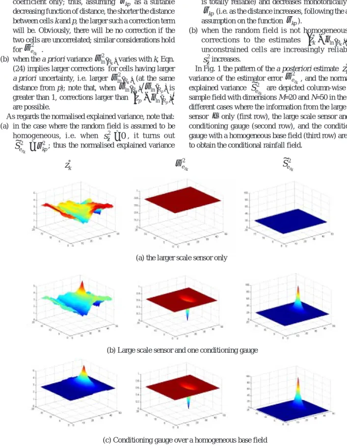
increases.

In Fig. 1 the pattern of the a posteriori estimate

z

*_k, the variance of the estimator error

σ

e2_zk , and the normalised

explained variance

~

2 k z

e

S

are depicted column-wise for a sample field with dimensions M=20 and N=50 in the three different cases where the information from the large scale sensor

χ

only (first row), the large scale sensor and one conditioning gauge (second row), and the conditioning gauge with a homogeneous base field (third row) are used to obtain the conditional rainfall field.

Fig. 1. Comparison of the spatial variability of z*_k, 2

k z e σ and ~2 k z e

S in a sample case where a) the larger scale sensor only, b) the larger scale sensor and one conditioning gauge, and c) the conditioning gauge over a homogeneous base field, are used for reconstruction field.

* k

z

2 k z e

σ

~

2 k z e

S

(c) Conditioning gauge over a homogeneous base field (b) Large scale sensor and one conditioning gauge

Consider now a given sub-grid partition of the target region both in time, using '

_/

τ

T

T

=

∆

∆

, and space, using 2 '

/

δ

y

x

S

=

∆

⋅

∆

∆

, which leads to the new grid dimensions

_m

=

δ

⋅

_M

and

_n

=

δ

⋅

_N

with δ > 1 and τ>1 (see Fig. 2). Again, a random variable

R

h

(

h

=

1

,....,

m

⋅

n

)

can be associated with each sub-grid cell to represent the stochastic rainfall process, R, at each location. The rain-gauge measurements are now attributed to the corresponding sub-grid cells using the proper area reduction factor, which is a function of the cell size. The expected value and variance of the random variable

h

R

are now derived from :

[ ]

R

r

h

P

( )

k

E

k h Rh

=

=

τ

∀

∈

µ

(27)

( )

k

P

h

CV

h h R R

=

⋅

∀

∈

2 2 2

µ

σ

(28)

where

r

_k is the kth _{element of}

( )

* 1

,

r

r

r

=

, P(k) = {sub-grid cells belonging to the kth _{cell at larger scale} and CV is}

the coefficient of variation.

The covariance matrix of Z =

(

Z

₁

,

Z

₂

,....,

Z

_m⋅n

)

— the new log-rainfall process at sub-grid scale — can also be evaluated, so that the a posteriori estimate of the rain field at the larger scales acts here as the a priori estimate of the sub-grid scale process in all ungauged locations. It is also possible to define the stochastic log-rainfall process

(

Z

1

, Z

2

)

Z

=

=

(

Z

1

,....,

Z

_G

,

Z

_G+1

,...,

Z

_m⋅n

)

(29)

and, therefore, obtain the joint probability distribution of

(

Z

2

| z

1

)

, conditional on the G rain-gauge measurements

at sub-grid scale.

To calibrate the mappings defined by Eqns. (1) and (2) and validate the proposed procedure, it would be necessary to run several experiments with varying model parameters

and finally compare the estimated conditional rainfall fields with that observed. Unfortunately, such rigorous validation is never possible, due to the common lack of any direct measurements of spatially distributed rain fields. Indirect methods are, therefore, usually addressed to perform both calibration and validation exercises.

One possible technique for the evaluation of random field estimates, known as the jacknife method, is based on alternately suppressing one out of the available conditioning sensors at the ground and evaluation, for each generated conditional rain field, of the marginal probability distribution of the random variable

R

j at the corresponding grid cell.

This is compared with the measured value at that cell and the procedure is repeated recursively for all the G nodes where a rain gauge is located (see Papamichail and Metaxa, 1996).

The procedure for conditional generation is therefore evaluated on the basis of the following performance index:

∑

=

=

G j j

e

G

MSE

1

1

(30) where

-

e

_j

=

(

r

_j

−

r

_j*

)

2 is the error reduction at each cell j where a sensor is located;

-

r

j is the “ground truth” measured at cell j;

-

r

*_j is the rainfall estimate at location j when measurement

r

j is neglected;

The calibration parameters are contained in the functions

( )

x

k

f

and

g

( )

x

_k , used to transform the measurements provided by the large scale sensor

χ

into the a priori mean and variance of the random field, and in the selected model for the correlation function

ρ

_ij. Application of the validation procedure to the reconstruction of a real rain field is described later with reference to the case study analysed.

Fig. 2. Conceptual scheme of the downscaling procedure

∆ Gauged cell ∆S ∆T ∆T′ ∆T′ ∆S′ ∆S′ δ = 4 τ = 2 N = 2 M = 2 n = 8 m = 8

A case study

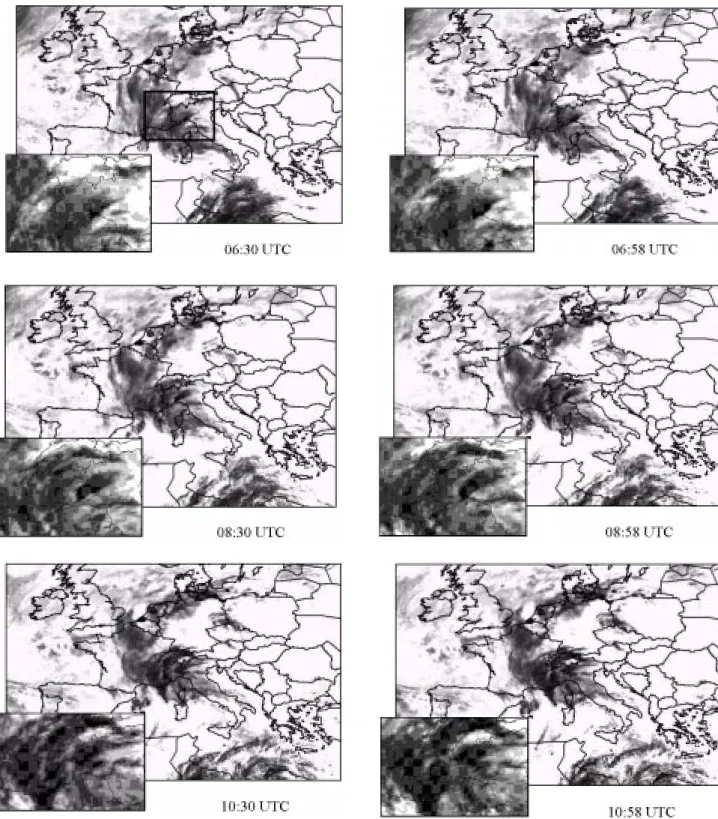
For the storm event on May 28th _{1998 in northern Italy, the}

meteorological situation at synoptic scale is well described by the Meteosat imagery in the thermal infrared (IR) band. A sequence of such images is provided in Fig. 3

corresponding to the core of the event over the Liguria region of Italy (see zoomed boxes).

The event analysed is embedded in a large-scale synoptic disturbance associated with a pressure low located over north-west Europe and producing a flow of humid air rising

Fig. 3. Sequence of IR Meteosat images from 06.30 to 10.58 UTC for the event of May 28th 1998 over Europe and zoomed over northern Italy

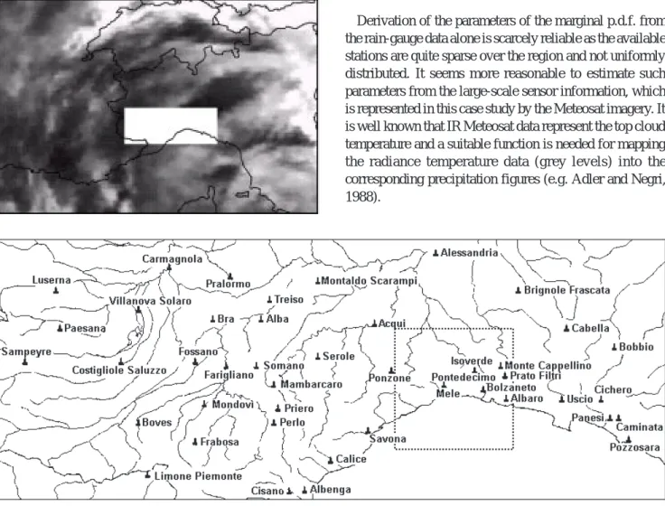
Fig. 4. Location of the study area and distribution of the available rain gauges. The dotted square denotes the area where

downscaling is applied.

from the south of the Mediterranean Sea towards the coastal European regions. Such meteorological conditions persist for a few days due to the blocking mechanism caused by a wide high located over Eastern Europe.

During the evolution of the event, humid airflows impinge on the west coast of Liguria causing strong low level convergence at local scales and intense precipitation over the study area in the time window 05:00 to 16:00 UTC, .

Low level convergence is associated with areas where the highest precipitation is observed, with values up to 100 mm in six hours, with the maximum rain rates at the ground being recorded at Mele, reaching 47 mm h–1_{. The location}

of the study area and the distribution of the available rain gauges are shown in Fig. 4 . The space-time distribution of rainfall has been determined over the study area (about 25 000 km2_{) by using 44 active rain-gauges from the local}

Hydrographic Service, most of them providing cumulated rainfall in hourly intervals.

The rain field has been discretised using a regular mesh of 50×18 pixels, each a square of side 5 km. To be coherent with the temporal resolution of the rain-gauge information, hourly data have been used for reconstruction of the rain field at the original space scale (therefore after aggregation of the half-hourly original Meteosat images). For the sake of brevity, only results referring to a single time slot (09:00 UTC) are shown here.

Similarly, rain-gauge rainfall fluctuations have been made coherent with the spatial resolution of the Meteosat images by application of appropriate area reduction factors to comply with the adopted pixel size.

To apply the proposed procedure for reconstruction of the precipitation field the following parameters must be specified: 1. second-order description (

µ

R_k , 2 k R

σ

) of the marginal p.d.f.

(

,

2

)

k k R R

LN

µ

σ

for

k

=

1

,....,

900

;

2. correlation coefficients

ρ

ij

(

i

,

j

=

1

,...,

900

)

for the

precipitation field.

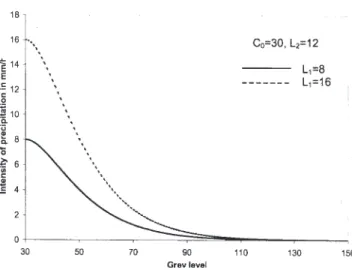
Derivation of the parameters of the marginal p.d.f. from the rain-gauge data alone is scarcely reliable as the available stations are quite sparse over the region and not uniformly distributed. It seems more reasonable to estimate such parameters from the large-scale sensor information, which is represented in this case study by the Meteosat imagery. It is well known that IR Meteosat data represent the top cloud temperature and a suitable function is needed for mapping the radiance temperature data (grey levels) into the corresponding precipitation figures (e.g. Adler and Negri, 1988).

The mapping of the Meteosat measurements (for each single pixel) to the mean values

µ

R_k

=

E

[ ]

R

k has been

obtained by using the following relationship:

( )

⋅

_



−

−

_











+

−

⋅

=

2 0 2 0 1

1

exp

L

C

x

L

C

x

L

x

f

k k k ₍₃₁₎

where C₀ is the grey level threshold, L₂ is the shape parameter and L₁ is a suitable coefficient (see Fig. 5).

The above relationship may be considered as a suitable continuous refinement of the empirical rule proposed by Adler and Negri (1988). A constant CV (equal to 1) has been assumed, so that

( )

(

( )

)

2

k

k

CV

f

x

x

g

=

⋅

(32)

As for the dependence of the spatial correlation coefficient on the distance, the following decay model has been used:









₋

=

γ

ρ

ij ij

d

exp

₍₃₃₎

with

d

ij the Euclidean distance between pixels i and j.

Calibration of the coefficients in functions (31) and (33) has been performed by estimating the MSE for a series of sets of parameter values. In Table 1 a synthesis of such results obtained is reported, as regards the calibration of parameter

γ

.

Table 1. Results for the case study analysed with C₀ =30,

8

1=

L andL₂ =12

γ

=0

γ

=1

ã

=2

γ

=3

γ

=4

γ

=8

MSE 3032 2405 1935.1 2134.3 3056 3537.2

From repeated experiments the set of parameter values which allows the most reliable reconstruction of the rainfall field corresponds to

C

₀

=

30

,

L

1

=

8

,

L

2

=

12

and

2

=

γ

. The reconstructed rain field r obtained by integration of the data from the two sensors (with parameters

30

0

=

C

,

L

₁

=

8

,

L

₂

=

12

and

γ

=

2

) and the map of standard deviations

(

k

M

N

)

k r e

=

1

,...,

⋅

2

σ

of the

random variables for the reconstructed field are shown in Figs. 6 and 7. In Fig. 8 the reliability map is presented for

the derived rain field.

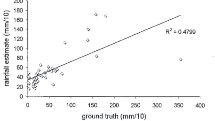
The observed ground truth and the estimate of the rain figures are compared in Figs. 9 to 12. In Fig. 9 rain estimates from Meteosat data, using (31) with parameters

C

0

=

30

,

8

1

=

L

,

L

2

=

12

, and rain-gauge data are compared. In

Fig. 10 the rain figures obtained with the proposed procedure using a base homogeneous field (the mean value of rain-gauge measurements) are compared with the rain-rain-gauge observations.

In Fig. 11 the rain figures obtained with the proposed procedure using Meteosat data with the set of parameters selected (

C

₀

=

30

,

L

1

=

8

,

L

2

=

12

and

γ

=

2

), are compared with the available ground truth, while in Fig. 12 the same graph is presented where a single outlier — which can be due to some measurement error — is eliminated.

The proposed procedure seems to provide the best performances when integration of Meteosat data and rain-gauge measurements is addressed. This reflects the obvious observation that the additional information contained in Meteosat data does contribute to a better rain field reconstruction than the use of rain-gauge measurements alone (homogeneous field). The scatterplot in Fig. 12 is obtained by eliminating the contribution of the station of Mele (see Fig. 2); note that the correlation obtained is about 0.8. The measurement in Mele can be considered an outlier if compared to the other instruments. Besides, this station is out of the influence zone of the other instruments and, when its contribution is neglected, the rain field information in that region only comes from the Meteosat images. It seems, therefore, reasonable to eliminate this information in the validation phase.

Downscaling of the reconstructed rain field has been possible thanks to the availability of high-resolution data from a sub-set of the available rain-gauges. Data with resolution in time of 15 minutes have been used and the sub-grid scale distribution of rainfall has been determined down to a spatial scale of about 3 km2 _{(1/9 of the original}

scale). The sub-region already identified in Fig. 6 where the highest rain rates were observed in the case study analysed, has been resized with a finer grid and the mean values at the former scale have been used for determination of the parameters of the new joint probability density

Fig. 5. Mapping from Meteosat data (grey levels) to rain mean value

using Eqn. 31 with sample parameters.

(

k M N

)

S

k

z =1,...., ⋅

Fig. 6. Rainfall field r from Meteosat data constrained to rain-gauge

Fig. 7. Standard deviation (_{k M N})

k r

e =1,..., ⋅

2

σ of rain fluctuations with respect to the Meteosat field constrained to rain-gauge

Fig. 8. Reliability map _S (_{k M N})

k

z =1,...., ⋅

function at the finer scale. The same procedure is then used for determination of the rainfall field at a finer scale, constrained at point values (five rain-gauges available) at the corresponding new time scale.

The scatterplot in Fig. 13 is analogous to those in Figs. 9–12, though the scarce number of rain-gauges available reduces the significance of the validation exercise in this context.

Obviously, downscaling increases the explained variance

of the process with respect to that obtained at the original scale. However, the variance of the rain field at finer scale is greater than the variance at the original scale. Therefore, with respect to the total variance, the explained variance decreases provided any additional information at finer scales (e.g. radar rain fields) is included.

In the first column of Fig. 14 the rainfall fields at 15-minute intervals obtained after downscaling the 1-hour field are shown while in the second column, maps of the standard deviation for the random variables of the reconstructed fields are reported.

Conclusions

Rain field reconstruction and downscaling procedures have been proposed for integration of rainfall data coming from different sources. Each of them provides different information in terms of reliability and scale. The procedures presented lead to the following results:

(1) mapping of the expected values of the reconstructed rainfall field at the same resolution of the available large scale information, using point data as a constraint; (2) mapping of the residual variance of the precipitation

Fig. 9. Meteosat data and ground truth Fig. 10. Estimate values using homogeneous field and ground truth

Fig. 11. Estimate values using Meteosat and ground truth Fig. 12. Same as in Fig. 11 with a single outlier eliminated

Fig. 14. Downscaling of the reconstructed rain field (on the left) and associated standard deviation maps (on the right)

process, i.e. a measure of the information content of the reconstructed rain field;

(3) quantitative evaluation of the reliability of the rainfall field at each cell of the grid.

The probabilistic information obtained about the rainfall field can be used for stochastic generation of different scenarios, with the purpose of determining the risk associated with specific space-time rainfall extremes in the region of concern, conditional on the available information on the specific rain event.

The procedure developed is based on the definition of various functions, which are used for conversion of the original information (as provided by the available sensors) into quantitative information about rainfall intensity, or better into suitable parameters characterising the probabilistic distribution of the rainfall field. Obviously, validation of such functions and their parameters is needed by means of an extensive comparison with actual rainfall measurements in a large number of case studies under various climatological conditions.

Throughout the paper we have assumed a constant CV over the whole rain field. The method can be modified easily to account for variable CV, provided some physical meaning is associated with the variability of these parameters. One possibility is to investigate the role of local precipitation-enhancing mechanisms in the study area and to model them e.g. orographic forcing through suitable patterns (maps) of CVs. This could be valuable in the downscaling frameworks as it allows one to include small-scale sources of variability in the process which are not yet captured by the large-scale observations or the individual point measurements of rainfall.

Further important features of space-time rainfall are not fully resolved by the proposed rain field reconstruction model, such as the bursting nature of rainfall with fractional coverage and alternate rain / no rain periods. In the approach presented, the modelling of such features is limited and reduced to the pattern that can be observed by the available rain-gauges. In the case of a sparse network, the fractional pattern between contiguous rain-gauges cannot be accounted for in this model. Future developments, possibly in synergy with intermittent models of space-time rainfall (e.g. Lanza, 2000) may allow integration of such modelling capabilities. This should proceed in parallel with the development of enhanced observing systems, such as radar networks, to obtain a measure of the space-time characteristics of fractional rain fields.

Acknowledgements

This work has been partially funded by the Italian MURST under the national project “Climatic and Anthropogenic Effects on Hydrological Processes”. It has also been partially funded by the National Group for Prevention from Hydrogeological Disasters (GNDCI) of the Italian National Council of Research (CNR).

References

Adler, R.F. and Negri, A.J., 1988. A satellite infrared technique to estimate tropical convective and stratiform rainfall, J. Clim.

Appl. Meteorol., 27, 30–51.

Bacchi, B. and Borga, M., 1993. Spatial correlation patterns and rainfall fields analysis, Excerpta, 7, 7–40.

Bastin, G. and Gevers, M., 1985. Identification and optimal estimation of random fields from scattered point-wise data,

Automatica, 21, 139–155.

Barancourt, C., Creutin, J.D. and Rivoirard, J., 1992. A method for delineating and estimating rainfall fields, Water Resour. Res.,

28, 1133–1144.

Barrett, E.C. and Beaumont, M.J., 1994. Satellite rainfall monitoring: an overview, Remote Sensing Reviews, 11, 23–48. Barrett, E.C. and Martin, D.W., 1981. The use of satellite data in

rainfall monitoring, Academic Press, London.

Box, G.E.P., Jenkins, G.M. and Reinsel, G.C., 1994. Time Series

Analysis (Forecasting and Control), Prentice-Hall, New Jersey.

Delrieu, G., Bellon, A. and Creutin, J.D., 1988. Estimation de lames d’eau spatiales à l’aide de données de pluviomètres et de radar météorologique - Application au pas de temps journalier dans la région de Montréal, J. Hydrol., 98, 315–344.

Krajewski, W.F., 1987. Cokriging radar-rainfall and rain gage data,

J. Geophys. Res., 92, 9571–9580.

Lanza, L.G., 2000. A conditional simulation model of intermittent rain fields, Hydrol. Earth Sys. Sci., 4, 173–183.

Papamichail, D.M. and Metaxa, I.G., 1996. Geostatistical analysis of spatial variability of rainfall and optimal design of a rain gauge network, Water Resour. Manag., 10, 107–127.

Seo, D.J., Krajewski, W.F. and Bowles, D.S. 1990a. Stochastic interpolation of rainfall data from rain gages and radar using cokriging – 1 – Design of experiments, Water Resour. Res., 26, 469–477.

Seo, D.J., Krajewski, W.F., Azimi-Zonooz, A. and Bowles, D.S., 1990b. Stochastic interpolation of rainfall data from rain gages and radar using cokriging – 2 – Results, Water Resour. Res., 26, 915–924.

Seo, D.J., 1998a. Real-time estimation of rainfall fields using rain gage data under fractional coverage conditions, J. Hydrol., 208, 25–36.

Seo, D.J., 1998b. Real-time estimation of rainfall fields using radar rainfall and rain gage data, J. Hydrol., 208, 37–52.

Sevruk, B. and Lapin, M., 1993. Precipitation Measurement and

Quality Control. Proc. Symp. on Precipitation and Evaporation,

Slovak Hydromet. Institute, Bratislava and Swiss Federal Inst. of Technology, Dep. of Geography, Zurich.