Biotic pump of atmospheric moisture as driver of the hydrological cycle on land

HAL Id: hal-00305066

https://hal.archives-ouvertes.fr/hal-00305066

Submitted on 27 Mar 2007

HAL is a multi-disciplinary open access

archive for the deposit and dissemination of

sci-entific research documents, whether they are

pub-lished or not. The documents may come from

teaching and research institutions in France or

abroad, or from public or private research centers.

L’archive ouverte pluridisciplinaire HAL, est

destinée au dépôt et à la diffusion de documents

scientifiques de niveau recherche, publiés ou non,

émanant des établissements d’enseignement et de

recherche français ou étrangers, des laboratoires

publics ou privés.

hydrological cycle on land

A. M. Makarieva, V. G. Gorshkov

To cite this version:

A. M. Makarieva, V. G. Gorshkov. Biotic pump of atmospheric moisture as driver of the hydrological

cycle on land. Hydrology and Earth System Sciences Discussions, European Geosciences Union, 2007,

11 (2), pp.1013-1033. �hal-00305066�

www.hydrol-earth-syst-sci.net/11/1013/2007/ © Author(s) 2007. This work is licensed under a Creative Commons License.

Earth System

Sciences

Biotic pump of atmospheric moisture as driver of the hydrological

cycle on land

A. M. Makarieva and V. G. Gorshkov

Petersburg Nuclear Physics Institute, Gatchina, St. Petersburg, Russia

Received: 31 March 2006 – Published in Hydrol. Earth Syst. Sci. Discuss.: 30 August 2006 Revised: 15 March 2007 – Accepted: 15 March 2007 – Published: 27 March 2007

Abstract. In this paper the basic geophysical and ecologi-cal principles are jointly analyzed that allow the landmasses of Earth to remain moistened sufficiently for terrestrial life to be possible. 1. Under gravity, land inevitably loses water to the ocean. To keep land moistened, the gravitational wa-ter runoff must be continuously compensated by the atmo-spheric ocean-to-land moisture transport. Using data for five terrestrial transects of the International Geosphere Biosphere Program we show that the mean distance to which air fluxes can transport moisture over non-forested areas, does not ceed several hundred kilometers; precipitation decreases ex-ponentially with distance from the ocean. 2. In contrast, pre-cipitation over extensive natural forests does not depend on the distance from the ocean along several thousand kilome-ters, as illustrated for the Amazon and Yenisey river basins and Equatorial Africa. This points to the existence of an ac-tive biotic pump transporting atmospheric moisture inland from the ocean. 3. Physical principles of the biotic mois-ture pump are investigated based on the previously unstudied properties of atmospheric water vapor, which can be either in or out of aerostatic equilibrium depending on the lapse rate of air temperature. A novel physical principle is formulated according to which the low-level air moves from areas with weak evaporation to areas with more intensive evaporation. Due to the high leaf area index, natural forests maintain high evaporation fluxes, which support the ascending air motion over the forest and “suck in” moist air from the ocean, which is the essence of the biotic pump of atmospheric moisture. In the result, the gravitational runoff water losses from the optimally moistened forest soil can be fully compensated by the biotically enhanced precipitation at any distance from the ocean. 4. It is discussed how a continent-scale biotic water pump mechanism could be produced by natural selection act-ing on individual trees. 5. Replacement of the natural forest

Correspondence to: A. M. Makarieva

(elba@infopro.spb.su)

cover by a low leaf index vegetation leads to an up to tenfold reduction in the mean continental precipitation and runoff, in contrast to the previously available estimates made without accounting for the biotic moisture pump. The analyzed body of evidence testifies that the long-term stability of an intense terrestrial water cycle is unachievable without the recovery of natural, self-sustaining forests on continent-wide areas.

1 Is it a trivial problem, to keep land moistened? Liquid water is an indispensable prerequisite for all life on Earth. While in the ocean the problem of water supply to liv-ing organisms is solved, the landmasses are elevated above the sea level. Under gravity, all liquid water accumulated in soil and underground reservoirs inevitably flows down to the ocean in the direction of the maximum slope of continental surfaces. Water accumulated in lakes, bogs and mountain glaciers feeding rivers also leaves to the ocean. So, to ac-cumulate and maintain optimal moisture stores on land, it is necessary to compensate the gravitational runoff of water from land to the ocean by a reverse, ocean-to-land, moisture flow.

When soil is sufficiently wet, productivity of plants and ecological community as a whole is maximized. With nat-ural selection coming into play, higher productivity is asso-ciated with higher competitive capacity. Thus, evolution of terrestrial life forms should culminate in a state when all land is occupied by ecological communities functioning at a max-imum possible power limited only by the incoming solar ra-diation. In such a state local stores of soil and underground moisture, ensuring maximum productivity of terrestrial eco-logical communities, should be equally large everywhere on land irrespective of the local distance to the ocean. Being determined by the local moisture store, local loss of water to river runoff per unit ground surface area should be distance-independent as well. It follows that in the stationary state the

amount of locally precipitating moisture, which is brought from the ocean to compensate local losses to runoff, should be evenly distributed over the land surface.

In the absence of biotic control, air fluxes transporting ocean-evaporated moisture to the continents weaken expo-nentially as they propagate inland. The empirically estab-lished characteristic scale length on which such fluxes are damped out is of the order of several hundred kilometers, i.e. much less than the linear dimensions of the continents. Geophysical atmospheric ocean-to-land moisture fluxes can-not therefore compensate local losses of moisture to river runoff that, on forested territories, are equally high far from the ocean as well as close to it. This means that no purely geophysical explanation can be given to the observed exis-tence of highly productive forest ecosystems on continent-scale areas of the order of tens of millions square kilometers, like those of the Amazonia, Equatorial Africa or Siberia.

To ensure functioning of such ecosystems, an active mech-anism (pump) is necessary to transport moisture inland from the ocean at a rate dictated by the needs of ecological com-munity. Such a mechanism originated on land in the course of biological evolution and took the form of forest – a con-tiguous surface cover consisting of tall plants (trees) closely interacting with all other organisms of the ecological com-munity. Forests are responsible both for the initial accumu-lation of water on continents in the geological past and for the stable maintenance of the accumulated water stores in the subsequent periods of life existence on land. In this pa-per we analyze the geophysical and ecological principles of the biotic water pump transporting moisture to the continents from the ocean. It is shown that only intact contiguous cover of natural forests having extensive borders with large water bodies (sea, ocean) is able to keep land moistened up to an optimal for life level everywhere on land, no matter how far from the ocean.

The paper is structured as follows. In Sect. 2 the exponen-tial weakening of precipitation with distance from the ocean is demonstrated for non-forested territories using the data for five terrestrial transects of the International Geosphere Bio-sphere Program (Sect. 2.1); it is shown that no such weak-ening occurs in natural forests, which points to the existence of the biotic pump of atmospheric moisture (Sect. 2.2); how the water cycle on land is impaired when this pump is bro-ken due to deforestation is estimated in Sect. 2.3. In Sect. 3 the physical principles of the biotic pump functioning are in-vestigated. The non-equilibrium vertical distribution of at-mospheric water vapor associated with the observed vertical lapse rate of air temperature (Sect. 3.1) produces an upward directed force, termed evaporative force, which causes the ascending motion of air masses (Sect. 3.2), as well as the horizontal air motions from areas with low evaporation to ar-eas with high evaporation. This physical principle explains the existence of deserts, monsoons and trade winds; it also underlies functioning of the biotic moisture pump in natu-ral forests. Due to the high leaf area index, natunatu-ral forests

maintain powerful evaporation exceeding evaporation from the oceanic surface.

The forest evaporation flux supports ascending fluxes of air and “sucks in” moist air from the ocean. In the result, for-est precipitation increases up to a level when the runoff losses from optimally moistened soil are fully compensated at any distance from the ocean (Sect. 3.3). Mechanisms of efficient retention of soil moisture in natural forests are considered in Sect. 3.4. In Sect. 4 it is discussed how the continent-scale biotic pump of atmospheric moisture could be produced by natural selection acting on individual trees. In Sect. 5, based on the obtained results, it is concluded that the long-term stability of a terrestrial water cycle compatible with human existence is unachievable without recovery of natural, self-sustaining forests on continent-wide areas.

2 Ocean-to-land moisture transport on forested versus non-forested land regions

2.1 Moisture fluxes in the absence of biotic control Let F be the horizontal moisture flux equal to the amount of atmospheric moisture passing inland across a unit horizontal length perpendicular to the stream line per unit time, dimen-sion kg H2O m−1s−1. With air masses propagating inland to

a distance x from the ocean (x is measured along the stream line), their moisture content decreases at the expense of the precipitated water locally lost to runoff. Thus, change of F per unit covered distance is equal to local runoff. In the ab-sence of biotic effects, due to the physical homogeneity of the atmosphere, the probability that water vapor molecules join the runoff, should not depend on the distance traveled by these molecules in the atmosphere. It follows that the change dF of the flux of atmospheric moisture over distance

dx should be proportional to the flux itself: R(x)≡dF (x) dx =− 1 lF (x) or F (x)=F (0) exp{− x l}, (1)

where R(x) is the local loss of water to runoff per unit sur-face area, kg H2O m−2s−1, l is the mean distance traveled by

an H2O molecule from a given site to the site where it went

to runoff, F (0) is the value of flux F in the initial point x=0. Parameter l reflects the intensity of precipitation formation processes (moisture upwelling, condensation and precipita-tion) (Savenije, 1995); the more rapid they are, the shorter the distance l. Moisture recycling (evaporation of water pre-cipitated on land) is also accounted for in the magnitude of parameter l.

As far as a certain amount, E, of the precipitated water evaporates from the surface and returns to the atmosphere, precipitation P is proportional to, and always higher than, runoff R and can be related to the latter with use of multiplier

k (Savenije, 1996a):

For example, global runoff constitutes 35% of terrestrial pre-cipitation (Dai and Trenberth, 2002), which gives a global mean multiplier k≈3. Equation (1) can then be re-written as

P (x) = P (0) exp{−x

l} or lnP (x) = lnP (0) − x

l, (3)

where P (0)=kR(0) is precipitation in the initial point x=0. Precipitation is maximal at x=0 and declines with increasing

x.

Linear scale l can be determined from the observed de-cline of precipitation P with distance x on those territories where the biotic control of water cycle is weak or absent al-together. Such areas are represented by arid low-productive ecosystems with low leaf area index, open canopies and/or short vegetation cover (semideserts, steppes, savannas, grass-lands). We collected data on five extensive terrestrial regions satisfying this criterion, i.e. not covered by natural close-canopy forests, Fig. 1. These regions represent the non-forested parts of five terrestrial transects proposed by the In-ternational Geosphere Biosphere Program (IGBP) for study-ing the effects of precipitation gradients under global change (Canadell et al., 2002), Table 1. Within each region distance

x was counted in the inland direction approximately

perpen-dicular to the regional isohyets (Savenije, 1995), Fig. 1. Based on the available meteorological data, the depen-dence of precipitation P on distance x was investigated in each region, Fig. 2a. In all regions this dependence accu-rately conforms to the exponential law Eq. (3), which is man-ifested in the high values of the squared correlation coeffi-cients (0.90–0.99), Table 1. This indicates that the possi-ble dependence on x of multiplier k, Eq. (2), which we do not analyze, is weak compared to the main exponential de-pendence of precipitation P on distance, which is taken into account in Eq. (3). Estimated from parameter b of the linear regression ln P =a+bx as l=−1/b, see Eq. (3), scale length l takes the values of several hundred kilometers, from 220 km in Argentina at 31◦S to 870 km in the North America, ex-cept for region 4a in Argentina at 45◦S, where l=93 km, Ta-ble 1. Such a rapid decrease of precipitation has to do with the influence of the high Andean mountain range impeding the movement of westerly air masses coming to the region from the Pacific Ocean (Austin and Sala, 2002). On the is-land of Hawaii, high (>4 km a.s.l.) mountains also create a large gradient of precipitation which can change more than tenfold over 100 km (Austin and Vitousek, 2000). In West Africa, the value of l=400 km obtained for the areas with

P ≤1200 mm year−1, Table 1, compares well with the re-sults of Savenije (1995), who found l ≈970 km for areas with

P ≥800 mm year−1and l∼300 km for the more arid zones of this region.

Total amount of precipitation 5 (kg H2O year−1) over the

entire path L≫l traveled by air masses to the inner parts of the continent, 0≤x≤L, in an area of width D (for river basins

Fig. 1. Geography of the regions where the dependence of

precip-itation P on distance x from the source of moisture was studied. Numbers near arrows correspond to regions as listed in Table 1. Ar-rows start at x=0 and end at x=xmax, see Table 1 for more details.

D can be approximated by the smoothed length of the coastal

line) is, due to Eq. (3), equal to

5 = D Z L

0

P (x)dx ≈ P (0)lD. (4) As is clear from Eq. (4), l represents a characteristic linear scale equal to the width of the band of land adjacent the coast which would be moistened by the incoming oceanic air masses if the precipitated moisture were uniformly dis-tributed over x with a density P (0). For land areas with or-dinary orography (regions 1–3, 4b, 5) the mean value of l is about 600 km, Table 1, i.e. it is significantly smaller than the characteristic horizontal dimensions of the continents. Thus, in the absence of biotic control the transport of moisture to land would only be able to ensure normal life functioning in a narrow band near the ocean of a width not exceeding several hundred kilometers; the much more extensive inner parts of the continents would have invariably remained arid. Already at this stage of our consideration we come to the conclusion that in order to explain the observed existence of the exten-sive well-moistened continental areas several thousand kilo-meters in length (the Amazon river basin, Equatorial Africa, Siberia), where natural forests are still functioning (Bryant et al., 1997), it is necessary to involve a different, biotically controlled mechanism of ocean-to-land moisture transport. 2.2 Biotic pump of atmospheric moisture

Let us now consider the spatial distribution of precipitation on extensive territories covered by natural forests. As far as soil moisture content ultimately dictates life conditions for all species in the ecological community, functioning of the community should be aimed at keeping soil moisture at a stationary level optimal for life. Maintenance of high soil moisture content W (units kg H2O m−2=mm H2O) enables

the ecological community to achieve high power of func-tioning even when the precipitation regime is fluctuating. For example, transpiration of natural forests in the Amazon river basin, where soil moisture content is high throughout

Table 1. Precipitation on land P (mm year−1) versus distance from the source of moisture x (km) as dependent on the absence/presence of natural forests

Region Parameters of linear regression1ln P = a − bx

No Name x=0 x=xmax xmax, a±1 s.e. (b±1 s.e.) r2 P (0)≡ea, l≡1/b,

◦_Lat,◦_Lon ◦_Lat,◦_{Lon km ×10}3 _{mm year}−1 _km

Non-forested regions2

1 North Australia3 −11.3, 130.5 −25, 137 1400 7.37± 0.05 1.54± 0.06 0.96 1600 650 2 North East China4 42, 125 42, 107 1500 6.67± 0.08 1.24± 0.10 0.96 790 800 3 West Africa5 10, 5 25, 5 1650 7.28± 0.09 2.46± 0.09 0.99 1450 400 4a Argentina6, 45◦S −44.8, −71.7 −45, −69.8 150 6.36± 0.17 10.8± 2.0 0.90 580 93 4b Argentina6, 31◦S −31.3, −65.3 −31.7, −68.3 360 6.35± 0.12 4.57± 0.59 0.91 570 220 5 North America7 39.8, −96.7 41.2, −105.5 750 6.69± 0.04 1.15± 0.08 0.93 800 870

Natural forests8

6 Amason river basin9 0, −50 −5, −75 2800 7.76± 0.04 −0.05 ± 0.02 0.13 2300 −2×104 7 Congo river basin10 0, 9 0, 30 2300 7.56± 0.17 −0.10 ± 0.12 0.05 1900 −1×104 8 Yenisey river basin11 73.5, 80.5 50.5, 95.5 2800 6.06± 0.17 −0.01 ± 0.10 0.05 430 −1×104 Notes:

1_{Statistics are significant at the probability level p<0.0001 for regions 1, 2, 3 and 5; p=0.013 for region 4a and p<0.001 for region 4b;}

p≥0.05 for regions 6, 7 and 8 (i.e., there is no exponential dependence of P on x in these regions).

2_{Regions 1, 2, 3, 4 (a and b) and 5 correspond to the non-forested parts of the North Australian Tropical Transect, North East China}

Transect (NECT), Savannah on the Long-Term Transect, Argentina Transect and North American Mid-Latitude Transect of the International Geosphere Biosphere Program, respectively (Canadell et al., 2002).

3_{Precipitation data for x=0 (Prilangimpi, Australia) taken from Cook and Heerdegen (2001), all other data taken from Fig. 2a of Miller}

et al. (2001) assuming 1oLat.=110 km.

4_{Data taken for 42}◦_{N of NECT, because at this latitude NECT comes most closely to the ocean. Location of x=0 approximately corresponds}

to the border between forest and steppe zones; the dependence between P and x obtained from the location of isohyets taken from Fig. 3c of Ni and Zhang (2000) assuming 10◦Lon.=825 km at 42◦N.

5_{Southern border of the non-forested part of West Africa approximately coincides with the 1200 mm isohyet, hence the choice of x=0 at}

10◦N 5◦E, where P =1200 mm year−1. The dependence between P and x was obtained from the location of isohyets taken from Fig. 2 of Nicholson (2000) assuming 1◦Lat.=110 km.

6_{Data for region 4a and 4b taken from Table 1 of Austin and Sala (2002) and Figs. 1 and 2 of Cabido et al. (1993), respectively. In region}

4b atmospheric moisture comes from the Pacific Ocean (Austin and Sala, 2002), in region 4a the ultimate source of moisture is the Atlantic Ocean (Zhou and Lau, 1998), hence the opposite directions of counting x in the two regions.

7_{Data taken from Table 1 of Barrett et al. (2002), x calculated assuming 1}◦_{Lat.=110 km.}

8_{Precipitation values for the three regions covered by natural forests are taken from the data sets distributed by the University of New}

Hampshire, EOS-WEBSTER Earth Science Information Partner (ESIP) at http://eos-webster.sr.unh.edu. Regions 6 and 8 correspond to the Amazon (LBA) and Central Siberia Transect of IGBP, respectively (Canadell et al., 2002).

9_{Precipitation data taken from the gridded monthly precipitation data bank LBA-Hydronet v1.0 (Water Systems Analysis Group, Complex}

Systems Research Center, University of New Hampshire), time period 1960–1990, grid size 0.5×0.5 degrees (Webber and Wilmott, 1998); statistics is based on P values for 26 grid cells that are crossed by the straight line from x=0 to x=xmax, Fig. 1.

10_{The transect was chosen in the center of the remaining natural forest area in the Equatorial Africa (Bryant et al., 1997). Precipitation}

data taken from the gridded annual precipitation data bank of the National Center for Atmospheric Research (NCAR)’s Community Climate System Model, version 3 (CCSM3), time period 1870–1999, grid size 1.4×1.4 degrees; statistics is based on P values for 16 grid cells that are crossed by the straight line from x=0 to x=xmax, Fig. 1.

11_{Precipitation data taken from the gridded monthly precipitation data bank Carbon Cycle Model Linkage-CCMLP (McGuire et al., 2001),}

time period 1950–1995, grid size 0.5×0.5 degrees; statistics is based on P values for 20 grid cells that are crossed by the straight line from x=0 to x=xmax, Fig. 1.

the year (Hodnett et al., 1996), is limited by the incom-ing solar energy only. It increases durincom-ing the dry season when the clear sky conditions predominate (da Rocha et al., 2004; Werth and Avissar, 2004). Dry periods during the

veg-etative season in natural forests of higher latitudes neither bring about a decrease of transpiration (Goulden et al., 1997; Tchebakova et al., 2002). In contrast, transpiration of open ecosystems like savannas, grasslands or shrublands incapable

of maintaining high soil moisture content year round, drops radically during the dry season (Hutley et al., 2001; Kurc and Small, 2004).

Change of soil moisture content with time, dW/dt, is linked to precipitation P , evaporation E and runoff R via the law of matter conservation, dW/dt=P −E−R. In the stationary state after averaging over the year dW/dt=0 and runoff R is a function of W . Therefore, high amount of soil moisture implies significant runoff, i.e. loss of water by the ecosystem. In areas where neither the surface slope, nor soil moisture content depend on distance x from the ocean,

W (x)=W (0), loss of ecosystem water to runoff is spatially

uniform as well, R(x)=R(0).

When the soil moisture content is sufficiently high, tran-spiration is dictated by solar energy. Interception, both from the canopy, understorey and the forest floor, which can be more than 50% of the total evaporation (Savenije, 2004), is also dictated by solar energy. So if there is suf-ficient soil moisture, then total evaporation from dense for-est is constrained by solar radiation. Therefore, when x is counted along the parallel, on well-moistened continental areas we have E(x)=E(0), i.e. evaporation should not de-pend on the distance from the ocean. Coupled with constant runoff, R(x)=R(0), this means that precipitation P should similarly be independent of the distance from the ocean,

P (x)=E(0)+R(0)=P (0). When the considered area is

ori-ented, and x counted, along the meridian, evaporation in-creases towards the equator following the increasing flux of solar energy. In such areas, provided soil moisture content and runoff are distance-independent, precipitation must also grow towards the equator irrespective of the distance from the ocean. The conditions W (x)=W (0) and R(x)=R(0) are incompatible with an exponential decline of P (x).

We collected precipitation data for three extensive ter-restrial regions spreading along 2.5 thousand kilometers in length each and representing the largest remnants of Earth’s natural forest cover (Bryant et al., 1997). These are the Amazon basin, the Congo basin (its equatorial part) and the Yenisey basin, regions 6, 7 and 8 in Fig. 1. As can be seen from Fig. 2b, precipitation in the Amazon and Congo basins is independent of the distance from the coast at around 2000 mm year−1. In the Yenisey river basin, which has a meridional orientation, Fig. 1, precipitation increases with distance from the ocean from about 400 mm year−1 at the mouth to about 800 mm year−1on the upper reaches of the river, Fig. 2b.

Similar precipitation, P (0)=790 mm year−1, is registered at 125◦E in that part of the North East China Continental Transect (NECT) (region 2), which is closest to the Pacific Ocean, 400 km from the coast. In the meantime, the upper reaches of Yenisey river are about four thousand kilometers away from the Pacific Ocean, and about six thousand kilo-meters away from the Atlantic Ocean; in fact, it is one of the innermost continental areas on the planet, Fig. 1. Due to the low oceanic temperature in the region of their formation,

Fig. 2. Dependence of precipitation P (mm year−1) on distance x (km) from the source of atmospheric moisture on non-forested ter-ritories (a) and on terter-ritories covered by natural forests (b). Regions are numbered and named as in Table 1. See Table 1 for parameters of the linear regressions and other details.

Arctic air masses that dominate the Yenisey basin (Shver, 1976) are characterized by low moisture content (less than 8 mm of precipitable water in the atmospheric column com-pared to 16 mm in the Pacific Ocean at NECT (Randel et al., 1996). According to Eq. (1), this moisture content should decrease even further as these air masses move inland to the south.

In other words, if the modern territory of the forest-covered Yenisey basin were, instead, a desert with precipi-tation of the order of 100 mm year−1, this would not be sur-prising from the geophysical point of view (indeed, one is not surprised at the fact that the innermost part of NECT and other non-forested regions, Fig. 2a, are extremely arid). This could easily be explained by the character of atmospheric circulation and large distance from any of the oceans. In contrast, the existence of a luxurious water cycle (Yenisey is the seventh most powerful river in the world) as well as the southward increase of precipitation in this area is quite remarkable, geophysically unexpected and can only be explained by functioning of an active biotic mechanism

pumping atmospheric moisture from ocean to land. Similar biotic pumps should ensure high precipitation rates through-out the natural forests of the Amazon basin and Equatorial Africa.

It can be concluded, therefore, that all the largest and most powerful river basins must have formed as an outcome of the existence of forest pumps of atmospheric moisture. For-est moisture pump ensures an ocean-to-land flux of mois-ture, which compensates for the runoff of water from the optimally moistened forest soil. This makes it possible for forests to develop the maximally possible evaporation fluxes that are limited by solar radiation only. Thus, precipitation over forests increases up to the maximum value possible at a given constant runoff (i.e., multiplier k in Eq. (2), the pre-cipitation/runoff ratio, is maximized for a given R.) For-est moisture pump determines both the ultimate distance to which the atmospheric moisture penetrates on the continent from the ocean, as well as the magnitude of the incoming moisture flux per unit length of the coastal line. Dictated by the biota, both parameters are practically independent of the geophysical fluctuations of atmospheric moisture circulation. The biotic pumps of atmospheric moisture enhance precipi-tation on land at the expense of decreasing precipiprecipi-tation over the ocean. This should lead to the appearance of extensive oceanic “deserts” – large areas with low precipitation (see, e.g., Fig. 1 of Adler et al., 2001).

2.3 Deforestation consequences for the water cycle on land Let us denote as Pf(x)=Pf(0) the spatially uniform

distri-bution of precipitation over a river basin covered by natu-ral forest (low index f stands for forest), which spreads over distance L inland and over distance D along the oceanic coast. Total precipitation 5f on this territory is equal to

5f=Pf(0)LD, where the product LD=S estimates the area

occupied by the river basin. According to Eq. (4) and the results of Sect. 2.1, total precipitation 5d on a territory of

the same area S deprived of the natural forest cover (low index d stands for deforestation, desertification) is equal to

5d=Pd(0)ldD, where ld∼600 km. One thus obtains

5f

5d

= Pf(0)L Pd(0)ld

. (5)

Equation (5) shows that the deforestation-induced decrease in the mean regional precipitation P ≡5/S in a river basin of linear size L is proportional to L. For example, for the Amazon river basin L≈3×103km, which means that Ama-zonian deforestation would have led to at least a L/ ld≈

5-fold decrease of mean precipitation in the region. This ef-fect, i.e. a 80% reduction in precipitation, is several times larger than the available estimates that are based on global circulation models not accounting for the proposed biotic moisture pump. According to such model estimates, de-forestation of the Amazon river basin would have led to (5f−5d)/S=270±60 mm year−1 (±1 s.e., n=22 models)

(McGuffie and Henderson-Sellers, 2001), i.e. only 13% of the modern basin mean precipitation of 2100 mm year−1 (Marengo, 2004).

Reduction of the characteristic distance of the inland prop-agation of atmospheric moisture from L to ld≪L is not the

single consequence of deforestation. Impairment of the bi-otic moisture pump in the course of deforestation causes the ocean-to-land flux of atmospheric moisture via the coastal zone to diminish. In the result, the amount of precipitation

P (0) in the coastal zone decrease from the initial high

bi-otic value P (0)=Pf(0) down to P (0)=Pd(0)<Pf(0). As will

be shown in Sect. 3.3, in the case of complete elimination of the vegetation cover, precipitation in the coastal zone can be reduced practically to zero, Pd(0)=0, see Fig. 4a. In the

case when the natural forest is replaced by an open-canopy, low leaf area index ecosystem, cf. Fig. 4b,c in Sect. 3.3, the characteristic magnitude of reduction in P (0) can be esti-mated comparing the observed values of precipitation P (0) in the coastal zones of forested versus non-forested territories under similar geophysical conditions of atmospheric circula-tion. A good example is the comparison of the arid ecosys-tem in the northeast Brazil, the so-called caatinga, which re-ceives about Pd(0)=800 mm year−1 precipitation (Oyama

and Nobre, 2004), with the forested coast of the Amazon river basin, where Pf(0)>2000 mm year−1(Marengo, 2004),

which gives Pf(0)/Pd(0)>2.5. According to Eq. (5), the

cu-mulative effect of deforestation can amount to more than a tenfold reduction of the mean basin precipitation. The inner-most continental areas will be inner-most affected. For example, at x=1200 km (in the Amazon river basin this approximately corresponds to the city of Manaus, Brazil) local precipitation will decrease by Pf(x) Pd(x) =Pf(0) Pd(0) 1 exp(−x/ l)= 2.5 exp(−1200/600)=19 (6) times, while in Rio Branco, Brazil (x≈+2500 km) precipita-tion will decrease by 160 times, i.e. the internal part of the continent will turn to a desert. Total river runoff from the basin to the ocean, which is equal toRL

0 R(x)dx=5/ k, see

Eq. (2), will undergo the same or even more drastic changes as the total precipitation, Eq. (5), due to increase of multiplier

k in deserts, Eq. (2).

Ratio 5f/5d>10, Eq. (5), characterizes the power of the

biotic pump of atmospheric moisture: the biotically induced ocean-to-land moisture flux does not decrease exponentially with distance from the ocean and it is more than an order of magnitude larger than in the biotically non-controlled state. At any distance from the ocean and under any fluctuations of the external geophysical conditions this moisture flux pre-vents forest soil from drying. As follows from the above ra-tio, geophysical fluctuations of the precipitation regime can be no more than 10% as powerful as the biotic pump. Rel-ative fluctuations of river runoff are dictated by fluctuations in the work of the biotic pump, i.e. they do not exceed 10%

of its power either. This prevents floods in the forested river basin.

In the theoretical consideration of moisture recycling (Savenije, 1996b) precipitation P is ultimately related to the horizontal flux of moisture, which is considered as an abiotic geophysical constraint, an independent parameter; evapora-tion E is known to be affected by vegetaevapora-tion; and runoff R is the residual of P and E. This consideration, where both

P and R can be arbitrarily high or low, corresponding to

ei-ther droughts and floods, should hold well for non-forested regions like deserts, agricultural lands etc.

In the biotic pump consideration a different meaning is as-signed to the budget P =E+R. In the biotically controlled forest environment runoff R is determined by the biotically maintained high soil moisture, total evaporation E is dictated by solar energy, and precipitation P is biotically regulated (via the biotically regulated flux F ) to balance the equation. In this consideration it is clear that, as is also confirmed by observations, in natural forests neither floods nor disastrous diminishment of runoff can normally occur throughout the year. Summing up, the undisturbed natural forests create an autonomous cycle of water on land, which is decoupled from whatever abiotic environmental fluctuations. We will now consider the physical and biological principles along which this unique biotic mechanism functions.

3 Physical foundations of the biotic pump of atmo-spheric moisture

3.1 Aerostatic equilibrium, hydrostatic equilibrium and the non-equilibrium vertical distribution of atmospheric water vapor

In this section we describe a physical effect, which, as we show, plays an important role in the meteorological processes on Earth, but so far remains practically undiscussed in the meteorological literature.

Aerostatic equilibrium of a gas mixture like moist air means that change dpi of partial pressure pi of the i-th gas

over vertical distance dz is balanced by the weight of this gas in the atmospheric layer of thickness dz (Landau and Lifs-chitz, 1987):

−dpi

dz =ρig. (7)

If each gas in the mixture obeys Eq. (7), for the mixture as a whole one has

−dp dz =ρg; (8) p =Xpi, ρ = X ρi = X NiMi.

Here ρi (g m−3) and Ni(mol m−3) are mass density and

mo-lar density of the i-th gas at height z, Mi (g mol−1) is its

mo-lar mass, g=9.8 m s−2is the acceleration of gravity; p and ρ

are pressure and mass density of moist air as a whole, respec-tively. Equation (8) can be written for gases as well as liquids and is often called the equation of hydrostatic equilibrium. It should be stressed that while the fulfillment of Eq. (7) for each mixture constituent guarantees the fulfillment of Eq. (8) for mixture as a whole, the opposite is not true.

Atmospheric gases are close to ideal and conform to the equation of state for ideal gas:

pi =NiRT ≡ ρighi, hi ≡ RT Mig , p = N RT ≡ ρgh, h ≡ RT Mg, (9) N =XNi, M ≡ ρ/N,

where T is absolute air temperature at height z, R=8.3 J K−1 mol−1is the universal gas constant. Therefore, Eq. (7) and its solution can be written in the following well-known form (Landau and Lifschitz, 1987; McEwan and Phillips, 1975):

dpi dz = − pi hi , pi(z) = pisexp{− Z z 0 dz hi }, (10) where pis is partial pressure of the i-th gas at the Earth’s

surface.

Aerostatic equilibrium of the gas mixture as a whole can-not be written in the form of a single differential equation with exponential solution (10), as far as functions N (9) and ρ (8) depend in different ways on molar concentra-tions Ni. In the troposphere, according to observations (see,

e.g., McEwan and Phillips, 1975), gases of dry air have one and the same vertical distribution with molar mass Md=29

g mol−1 independent of height z. As far as pd/ hd=ρdg,

hd≡RT /(Mdg), hds=8.4 km, see Eq. (9), dry air obeys

Eq. (8) for hydrostatic equilibrium (if it is written for pdand

ρdinstead of p and ρ). But dry air is not in aerostatic

equilib-rium; vertical distribution of each particular i-th dry air con-stituent does not conform to Eqs. (7) and (10), eventhough vertical distribution of dry air as a whole (low index d) for-mally obeys Eqs. (10) at i=d. Moist air does not conform to either Eq. (7) or Eq. (8).

Aerostatic equilibrium of atmospheric water vapor (low index v) with molar mass Mv=18 g mol−1 is described

by Eq. (10) with i=v and hi replaced by hv≡RT /Mvg,

hvs≡RTs/Mvg=13.5 km.

Immediately above wet soil or open water surface, water vapor is in the state of saturation. The dependence of partial pressure pH2O of saturated water vapor on air temperature

T is governed by the well-known Clapeyron-Clausius law

(Landau et al., 1965): dpH2O dz = − pH2O hH2O , pH2O =pH2Osexp{− Z z 0 dz hH2O }, hH2O ≡ T2 {−dT dz}TH2O , TH2O≡ QH2O R ≈5300 K, (11)

where, as everywhere else, low index s refers to correspond-ing values at the Earth’s surface, QH2O≈44 kJ mol

−1_{is the}

molar latent heat of evaporization.

Equations (11) have the same form as the aerostatic equi-librium equations (10), but with a different height parameter

hH2O, which, in the case of water vapor, depends on the at-mospheric lapse rate Ŵ of air temperature, Ŵ≡−dT /dz.

Written for water vapor with hv instead of hi, Eqs. (10)

formally coincide with Eqs. (11) if the equality hH2O=hvis fulfilled. This equality can be solved for the atmospheric temperature lapse rate Ŵ. The obtained solution Ŵ=ŴH2O corresponds to the case when water vapor is saturated in the entire atmospheric column and at the same time is in aero-static equilibrium, i.e. at any height z its partial pressure is equal to the weight of water vapor in the atmospheric column above z. Equating the scale heights hv≡RT /Mvg, Eq. (10)

and hH2O, Eq. (11), we arrive at the following value of ŴH2O:

−dT dz = T H, T = Tse −z/H_, −dT dz ≡ŴH2O = Ts H =1.2 K km −1_{, (12)} H ≡ RTH2O Mvg =250 km.

Note that due to the large value of H ≫hv, hv/H ≈0.05≪1,

one can put exp(−z/H )≈1 for any z≤hv, which we did

when obtaining Eq. (12). In Eq. (12) ŴH2O=1.2 K km

−1

is calculated for the mean global surface temperature

Ts=288 K. Differences in the absolute surface temperatures

of equatorial and polar regions change this value by no more than 10%.

The obtained value of ŴH2O=1.2 K km

−1_{, Eq. (12), is}

a fundamental parameter dictating the character of atmo-spheric processes.

When Ŵ<ŴH2O, water vapor in the entire atmosphere is in aerostatic equilibrium, but it is saturated at the surface only, i.e. pv(z)<pH2O(T (z)) for z>0 and pv(z)=pH2O(Ts) for z=0, where pvis partial pressure of water vapor at height

z (and pH2O, as before, is the saturated pressure of water vapor at T (z)). Relative humidity pv/pH2Odecreases with height. As far as in the state of aerostatic equilibrium wa-ter vapor partial pressure pv, as well as partial pressures pi

of other air gases, at a given height z are compensated by the weight of these gases and water vapor in the atmospheric column above z, in this state macroscopic fluxes of air and water vapor in the atmosphere are absent. Evaporation and precipitation are zero at any surface temperature. Solar radi-ation absorbed by the Earth’s surface makes water evaporate from the oceanic and soil surface, but the evaporated water undergoes condensation at a microscopic distance above the surface, which is of the order of one free path length of water vapor molecules. Energy used for evaporation is ultimately released in the form of thermal radiation of the Earth’s sur-face, with no input of latent heat into the atmosphere.

At Ŵ>ŴH2O the situation is quite different. In this case atmospheric water vapor cannot be in aerostatic equilibrium, Eq. (7), in that part of the atmospheric column where it is saturated, i.e. where pv(z)=pH2O(T (z)). Due to the steep decline of air temperature with height, the atmospheric col-umn above z cannot bear a sufficient amount of water va-por for its weight to compensate saturated water vava-por par-tial pressure at height z. The excessive moisture condenses and precipitates. The lapse rate of water vapor partial pres-sure, −dpv/dz, is larger than the weight of a unit volume

of saturated water vapor, Eq. (7). There appears an uncom-pensated force acting on atmospheric air and water vapor. Under this force, upward fluxes of air and water vapor orig-inate that are accompanied by the vertical transport of latent heat. With water vapor continuously leaving the surface layer for the upper atmosphere, saturation of water vapor near the surface can be maintained by continuous evaporation and ad-vective (horizontal) inputs of water vapor. In the imaginary case when evaporation discontinues, all atmospheric water vapor ultimately condenses and the stationary global partial pressure of atmospheric water vapor will be zero. In contrast, at Ŵ<ŴH2Oany surface value of water vapor partial pressure

pvs≤pH2O(Ts) can be stationarily maintained in the absence of evaporation.

Violation of aerostatic equilibrium is manifested as a strong compression of the vertical distribution of water va-por as compared to the distribution of dry atmospheric air, Eq. (10) for i=d (d stands for dry air). At the observed mean atmospheric value of Ŵ=Ŵob=6.5 K km−1, see Appendix A,

we obtain from Eqs. (10), (11) and (12):

hd hH2O = Ŵob ŴH2O Mv Md Ts T ≡β ≡ βs Ts T , βs =3.5. (13)

The compression coefficient β grows weakly with z due to the z-dependent drop of temperature T corresponding to

Ŵob=6.5 K km−1. At z=hH2O, which defines the character-istic vertical scale of water vapor distribution, β increases by 5% compared to its value at the surface βs. Ignoring

this change and putting β constant at β=βs we obtain from

Eqs. (10), (11), and (13): pH2O(z) pH2Os =exp{− Z z 0 dz hH2O } = =exp{− Z z 0 βdz hd } ≈ {pd(z) pds }β. (14)

Equation (14) shows that the vertical distribution of water va-por in the troposphere is compressed 3.5-fold as compared to the vertical distribution of atmospheric air. Its scale height

hH2Osis calculated as hH2Os=hs/βs=2.4 km. This theoreti-cal theoreti-calculation agrees with the observed stheoreti-cale heights ≈2 km of the vertical profiles of atmospheric water vapor (Goody and Yung, 1989; Weaver and Ramanathan, 1995).

Let us now emphasize the difference between the physical picture that we have just described and the traditional con-sideration of atmospheric motions. The latter resides on the

notion of convective instability of the atmosphere associated with the adiabatic lapse rate Ŵa(dry or wet). If an air parcel

is occasionally heated more than the surrounding air, it ac-quires a positive buoyancy and, under the Archimedes force, can start an upward motion in the atmosphere. In such a case its temperature decreases with height z at a rate Ŵa. If the

environmental lapse rate Ŵ is steeper than Ŵa, Ŵ>Ŵa, the

rising parcel will always remain warmer and lighter that the surrounding air, thus infinitely continuing its ascent. Similar reasoning accompanies the picture of a descending air par-cel initially cooled to a temperature lower than that of the surrounding air. On such grounds, it is impossible to deter-mine either the degree of non-uniformity of surface heating responsible for the origin of convection, or the direction or velocity of the resulting movement of air masses. After av-eraging over a horizontal scale exceeding the characteristic height h of the atmosphere, mean Archimedes force turns to zero. This means that the total air volume above an area greatly exceeding h2cannot be caused to move anywhere by the Archimedes force.

According to the physical laws that we have discussed, up-ward fluxes of air and water vapor always arise when the environmental lapse rate exceeds ŴH2O=1.2 K km

−1_{. This}

critical value is significantly lower than either dry or wet adi-abatic lapse rates Ŵa(9.8 and ≈6 K km−1, respectively). The

physical cause of these fluxes is not the non-uniformity of atmospheric and surface heating, but the fact that water va-por is not in aerostatic equilibrium and its partial pressure is not compensated by its weight in the atmospheric column, Fig. 3a. The resulting force is invariably upward-directed, Fig. 3b. It equally acts on air volumes with positive and neg-ative buoyancy, in agreement with the observation that atmo-spheric air updrafts exhibit a wide range of both positive and negative buoyancies (Folkins, 2006). Quantitative consider-ation of this force, which creates upwelling air and water va-por fluxes and supva-ports clouds over large areas of the Earth’s surface, makes it possible to estimate characteristic veloci-ties of the vertical and horizontal motions in the atmosphere, which is done in the next sections.

3.2 Vertical fluxes of atmospheric moisture and air The Euler equation for the stationary vertical motion of moist air under the force fEgenerated by the non-equilibrium

pres-sure gradient of atmospheric water vapor can be written as follows (Landau and Lifschitz, 1987):

1 2ρ dw2 dz =− dp dz−ρg=− dpv dz −ρvg ≡ fE (15)

Here ρ=ρd+ρv and p=pd+pvare density and pressure of

moist air at height z, respectively; ρd, ρv and pd, pv are

density and pressure of dry air and water vapor at height z, respectively; w is vertical velocity of moist air at height z; it is taken into account that dry air is in hydrostatic equilibrium, i.e. −dpd/dz−ρdg=0.

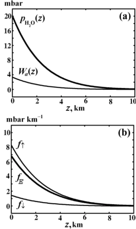
Fig. 3. Water vapor partial pressure and evaporative force in the terrestrial atmosphere. (a) Saturated partial pressure of water va-por pH2O(z), Eq. (11), and weight of the saturated water vapor

Wa(z)≡Rz∞ p_H2O(z′)

hv(z)′ dz

′_{in the atmospheric column above height}

z at Ŵob=6.5 K km−1. Saturated partial pressure at the surface is

pH2O(0)=20 mbar. (b) The upward-directed evaporative force fE,

Eq. (16), equal to the difference between the upward directed pres-sure gradient force f_↑(z) and the downward directed weight f_↓of a unit volume of the saturated water vapor, fE=f↑−f↓.

For saturated water vapor, pv=pH2O, under conditions of the observed atmospheric lapse rate Ŵob=6.5 K km−1,

when pH2Ois given by Eq. (11), we have from Eq. (15):

fE=− dpH2O dz − pH2O hv =pH2O( 1 hH2O −1 hv )= =(β−βv)ργ g. (16)

Here βv≡Mv/M≈0.62, β is given by Eq. (13), γ ≡pH2O/p is mixing ratio of saturated water vapor; hv=RT /Mvg.

Since γ ≪1, we put with a very good accuracy M=Md,

ρ=ρd.

Force fE, Eq. (16), acting on a unit moist air volume

is equal to the difference between the upward directed pressure gradient force f↑(z) associated with partial

pres-sure of the vertically compressed saturated water vapor,

f↑(z)≡−dpH2O(z)/dz=pH2O/ hH2O, and the downward di-rected weight f↓of a unit volume of the saturated water

va-por, f↓≡pH2O(z)/ hv: fE=f↑−f↓, Fig. 3b. Due to the ver-tical compression of water vapor as compared to the state of hydrostatic equilibrium of dry air, at any height z the pressure

of moist air, p=pd+pH2O, becomes larger than the weight of the atmospheric column above z, so force fE arises. Acted

upon by this upward directed force at any height z, volumes of moist air start to rise tending to compensate the insufficient weight of the atmospheric column above z.

As can be seen from Eq. (16), force fE is proportional

to the local concentration NH2O=pH2O/RT of the saturated water vapor. As far as the ascending water vapor molecules undergo condensation, the stationary existence of force fEis

only possible in the presence of continuous evaporation from the surface, which would compensate for the condensation. It is therefore natural to term force fE, Eq. (16), as the

evap-orative force.

As is well-known, the horizontal barometric gradient force accelerates air masses up to certain velocities when the rel-evant Coriolis force caused by Earth’s rotation comes into play. It grows proportionally to velocity and is perpendicu-lar to the velocity vector. These two forces along with the centrifugal force of local rotational movements, the turbulent friction force describing the decay of large air eddies into smaller ones, and the laws of momentum and angular mo-mentum conservation together explain the observed atmo-spheric circulation patterns like gradient winds in cyclones and anticyclones, cyclostrophic winds in typhoons and torna-does, as well as geostrophic winds in the upper atmosphere where turbulent friction is negligible. However, the origin, magnitude and spatial distribution of the horizontal baromet-ric gradient – the primary cause of atmosphebaromet-ric circulation – has not so far received a satisfactory explanation (Lorenz, 1967). Below we show that the observed values of the baro-metric gradient are determined by the magnitude of the evap-orative force. The various patterns of atmospheric circula-tion correspond to particular spatial and temporal changes in the fluxes of evaporation, so the evaporative force drives the global atmospheric circulation.

In agreement with Dalton’s law, partial pressures of differ-ent gases in a mixture independdiffer-ently come in or out of the equilibrium. The non-equilibrium state of atmospheric wa-ter vapor cannot bring about a compensating deviation from the equilibrium of the other air gases, to zero the evapora-tive force. (In such a hypothetical case the vertical distri-bution of air would be “overstretched” along the vertical, in contrast to the distribution of water vapor which is vertically compressed as compared to the state of aerostatic equilib-rium.) A non-equilibrium vertical distribution of air con-centration would initiate downward diffusional fluxes of air molecules working to restore the equilibrium. As soon as air molecules undergo a downward diffusional displacement, the weight of the upper atmospheric column diminishes ren-dering partial pressure of the water vapor uncompensated, and the evaporative force reappears. (A similar effect when a fluid-moving force arises in the course of diffusion of fluid mixtures with initially non-equilibrium concentrations is in-herent to the phenomenon of osmosis.) Thus, the only pos-sible stationary state in the case of non-equilibrium vertical

distribution of water vapor, Eq. (14), is the dynamic state when parcels of moist air move under the action of the evap-orative force. According to the law of matter conservation, movement trajectories should be closed for air molecules and partially closed (taking into account condensation and pre-cipitation of moisture) for the water vapor. The particular shape of these trajectories will be dictated by the boundary conditions.

Flux of H2O molecules through the liquid-gas interface is

determined by temperature only. At fixed temperature it is the same at Ŵ≤ŴH2O and Ŵ>ŴH2O. At Ŵ≤ŴH2O the evap-orative force is equal to zero; evaporation, i.e. flux of water vapor from the liquid water surface to the macroscopic at-mospheric layers, is absent; the temperature-dictated flux of H2O molecules from liquid to gas is compensated by the

re-verse flux of molecules from gas to liquid at a microscopic distance from the surface. At Ŵ>ŴH2Othe evaporative force is not zero; it “sucks” water vapor (and air) up to the atmo-sphere from the microscopic layer at the surface; there ap-pears a non-zero evaporation. The evaporative force acceler-ates moist air until the dynamic upward flux of water vapor

wNH2O becomes equal to the stationary evaporation flux E determined by solar radiation. After this value is reached at a certain (quite small) height z in the atmosphere, the ac-celeration starts to drop very rapidly with height, because local water vapor concentration drops below the saturated value, relative humidity becomes less than unity, water va-por tends to aerostatic equilibrium and the evava-porative force drops sharply, Eq. (15). In the result, vertical velocity of moist air can remain practically constant at any height in the atmospheric column. At some height of the order of hH2O, where water vapor reaches saturation, the evaporative force increases. In the stationary case it compensates for the fric-tion force acting on water droplets appearing in the course of water vapor condensation, thus maintaining clouds at a cer-tain height in the atmosphere, as well as for the friction force acting on the horizontally moving air at the surface.

In the stationary case the dynamic ascending flux of moist air removing wNH2Omol water vapor from unit surface area per unit time, where w is vertical velocity, should be com-pensated by the incoming flux K bringing moisture to the considered area, K=wNH2O. On the global average, K is fixed by flux E of evaporation from the Earth’s surface. For the global mean value of E≈103kg H2O m−2 year−1

≈55×103mol m−2 year−1 and saturated water vapor con-centration at the surface NH2Os=0.7 mol m

−3 _{at the global}

mean surface temperature Ts=288 K we obtain

w_E=E / NH2O=2.5 mm s

−1_{. (17)}

If K is determined by evaporation supported by advective heat fluxes or directly by the horizontal advective moisture inputs from the neighboring areas, its value can significantly exceed mean local evaporation E. In such a case vertical velocity of moist air movement under the action of the evap-orative force can reach its maximum value wmax, when the

evaporative force accelerates air parcels along the entire at-mospheric column. Using the expression for air pressure

p≈pdgiven by Eq. (10) for i=d, the approximate equality in

Eq. (14), and recalling that ρ=p/gh, one can estimate wmax

from Eq. (16) as wmax= [2(β − βv)gγs Z ∞ 0 dz exp{− Z z 0 (β −1)dz ′ h }] 1 2_≈ ≈p2γsghs ≈50 m s−1. (18) where γs≡pH2Os/ps≈2×10 2_{, h} s=8.4 km, g=9.8 m s−2.

The obtained theoretical estimate Eq. (18) is in good agreement with the maximum updraft velocities observed in typhoons and tornadoes (e.g. Smith, 1997). The value of

wmax, Eq. (18), exceeds the global mean upward velocity

w_E, Eq. (17), which is stationarily maintained by the global mean evaporation E at the expense of solar energy absorbed by the Earth’s surface, by ∼104 times. Such velocities can be attained if only there is a horizontal influx of water vapor and heat into the considered local area where the air masses ascend, from an adjacent area which is ∼104 times larger, i.e. from a distance one hundred of times greater than the characteristic maximum wind radius in tornadoes and hurri-canes.

Movement of air masses under the action of the evapora-tive force follow closed trajectories, which have to include areas of ascending, descending and horizontal motion. The vertical pressure difference 1pzassociated with the

evapora-tive force is equal to 1pz≈pH2O∼10

−2_p

s, where ps=105Pa

is atmospheric pressure at the Earth’s surface. The value of

1pz, about one per cent of standard atmospheric pressure,

should give the scale of atmospheric pressure changes at the sea level in cyclones and anticyclones; this agrees well with observations. Given that the scale length r of the areas with consistent barometric gradient does not exceed several thou-sand kilometers, at r∼103km the horizontal barometric gra-dient is estimated as ∂p/∂x∼1pz/r∼1 Pa km−1. Again, this

theoretical estimate agrees well with characteristic magni-tude of horizontal pressure gradients observed on Earth.

Taking into account that movement of air masses under the action of the evaporative force with a mean vertical ve-locity w_E, Eq. (17), is the cause of the turbulent mixing of the atmosphere, it is also possible to obtain a theoreti-cal estimate of the turbulent diffusion coefficient for the ter-restrial atmosphere. If there is a gradient of some variable

C in the atmosphere, the diffusion flux Fν of this variable

is described by the equation of turbulent (eddy) diffusion,

Fν=−ν[∂C/∂z−(∂C/∂z)0], where (∂C/∂z)0is the

equilib-rium gradient and the eddy (turbulent) diffusion coefficient

ν (m2s−1) (kinematic viscosity) does not depend on the na-ture of the variable or its magnitude. This relationship is for-mally similar to the equation of molecular diffusion. How-ever, molecular diffusion fluxes are caused by concentration gradients alone, with no forces acting on the fluid. Molecu-lar diffusion coefficient is unambiguously determined by the

physical properties of state, in particular, by the mean veloc-ity and free path length of air molecules. In contrast, turbu-lent fluxes are caused by air eddies that are maintained by certain physical forces acting on macroscopic air volumes and making them move; thus, the eddy diffusion coefficient depends on air velocity. Therefore, using the empirically es-tablished eddy diffusion coefficient for the determination of the characteristic air velocity via the scale length of the con-sidered problem, a common feature of many theoretical stud-ies of global circulation, e.g., (Fang and Tung, 1999), repre-sents a circular approach. It sheds no light on the physical nature and magnitude of the primary forces responsible for air motions.

As is well-known, eddy diffusion coefficient can be es-timated if one knows the characteristic velocity and linear scale of the largest turbulent eddies (Landau and Lifschitz, 1987). Theoretically obtained vertical velocity w_E, Eq. (17), and the scale height hH2O∼2 km of the vertical distribution of atmospheric water vapor make it possible to estimate the global mean atmospheric eddy diffusion coefficient (which, for atmospheric air, coincides with the coefficient of turbu-lent kinematic viscosity) as ν∼w_EhH2O∼6 m

2_s−1_{. This}

es-timate agrees in the order of magnitude with, but is about two times greater than, the phenomenological value of ν∼3.5 m2s−1 used in global circulation studies (Fang and Tung, 1999).

However, when obtaining the estimate of vertical velocity w_E, Eq. (17), it was assumed that the mean global flux of evaporation E is equal to the vertical dynamic flux Fw=wENH2O of water vapor, E=Fw, while in reality it is equal to the sum of the dynamic

Fw and eddy Fν fluxes of water vapor, E=Fw+Fν.

The upward eddy flux of water vapor is equal to

Fν=−ν[∂NH2O/∂z−(∂NH2O/∂z)0]=νh

−1

H2ONH2O(1−βv/β) =

w_ENH2O×0.82 at ν=wEhH2O. Thus, the account of eddy flux reduces the estimate of vertical veloc-ity w_E by 1.82 times, from w_E=E/Fw, Eq. (17), to

w_E=E/(Fw+Fν)=1.3 mm s−1. The resulting estimate of

the global mean eddy diffusion coefficient ν=3.3 m2 s−1 practically coincides with the phenomenological value. This lends further support to the statement that the observed turbulent processes in the atmosphere and atmospheric circulation are ultimately conditioned by the process of evaporation of water vapor from the Earth’s surface at the observed Ŵob=6.5 K km−1and are generated by the

evapo-rative force, Eq. (16). Finally, we note that the evapoevapo-rative force equally acts on all gases irrespective of their molar mass, so when the ascending air parcels expand, the relative amount of the various dry air components does not change. This explains the observed constancy of dry air molar mass

Md (i.e. constant mixing ratios of the dry air constituents)

3.3 Horizontal fluxes of atmospheric moisture and air Based on the physical grounds discussed in the previous two sections, it is possible to formulate the following physical principle of atmospheric motion. If evaporation fluxes in two adjacent areas are different, the ascending fluxes of moist air are different as well. Therefore, there appear horizon-tal fluxes of moist air from the area with weaker evaporation to the area where evaporation is more intensive. The result-ing directed moisture flow will enhance precipitation in the area with strong evaporation and diminish precipitation in the area with weak evaporation. In particular, it is possible that moisture will be brought by air masses from dry to wet areas, i.e. against the moisture gradient. This is equivalent to the existence of a moisture pump supported by the energy spent on evaporation. This pattern provides clues for several important phenomena.

First, it explains the existence of deserts bordering, like Sahara, with the ocean. In deserts where soil moisture stores are negligible, evaporation from the ground surface is prac-tically absent. Atmospheric water vapor is in the state of aerostatic equilibrium, Eq. (10), so the evaporative force, Eq. (16), in desert is equal to zero. In contrast, evaporation from the oceanic surface is always substantial. The upward-directed evaporative force is always greater over the ocean than in the desert. It makes oceanic air rise and effectively “sucks in” the desert air to the ocean, where it replaces the rising oceanic air masses at the oceanic surface, Fig. 4a. The reverse ocean-to-desert air flux occurs in the upper atmo-sphere, which is depauperate in water vapor. This moisture-poor air flux represents the single source of humidity in the desert. Its moisture content determines the stationary rela-tive humidity in the desert. To sum up, due to the absence of surface evaporation, deserts appear to be locked for oceanic moisture year round, Fig. 4a.

In less arid zones like savannas, steppes, irrigated lands, some non-zero evaporation from the surface is present throughout the year. Land surface temperature undergoes greater annual changes than does the surface temperature of the thermally inert ocean. In winter, the ocean can be warmer than land. In such a case partial pressure pH2Oof water vapor in the atmospheric column over the ocean is higher than on land. The evaporative force is greater over the ocean as well. In the result, a horizontal land-to-ocean flux of air and mois-ture originates, which corresponds to the well-known phe-nomenon of winter monsoon (dry season), Fig. 4b.

In contrast, as the warm season sets in, land surface heats up more quickly than does the ocean and, despite the preced-ing dry winter season, the evaporation flux from the land sur-face can exceed the evaporation flux over the colder ocean. There appears an air flux transporting oceanic moisture to land known as summer monsoon (rainy season), Fig. 4c. In the beginning, only the wettest part of land, the coastal zone, can achieve an evaporation flux in excess of the oceanic one. This initiates the fluxes of moist air, precipitation and

fur-ther enhances terrestrial evaporation. As the evaporation flux grows, so do the fluxes of moist air from the ocean. They gradually spread inland to the drier parts of the continent and weaken exponentially with distance from the ocean, see Eqs. (1), (3) and Fig. 2a. Notably, an indispensable condi-tion for summer monsoon is the considerable store of water on land, which sustains appreciable evaporation year round. In deserts, in spite of even greater seasonal differences be-tween land and ocean surface temperatures, the evaporation on land is practically absent, so no ocean-to-land fluxes of moisture can originate in any season.

Although the vegetation of savannas does support some non-zero ground stores of moisture and fluxes of evapora-tion, the absence of a contiguous cover of tall trees with high leaf area index prevents such ecosystems from increasing evaporation up to a level when the appearing flux of atmo-spheric moisture from the ocean would compensate runoff from the optimally moistened soil. The biotic pump of at-mospheric moisture does not work in such scarcely vege-tated ecosystems; precipitation weakens exponentially with distance from the ocean, Fig. 2a.

The phenomenon of trade winds (Hadley circulation) can also be explained on these grounds. As far as in the station-ary case solar radiation is the source of energy for evapora-tion, the increase of the solar flux towards the equator should be accompanied by a corresponding increase of evaporation flux E, evaporative force fE, Eq. (16), and vertical velocity

w, Eq. (17). The intensive ascent of moist air on the equator

has to be compensated by horizontal air fluxes originating at higher latitudes and moving towards the equator, where they ascend and travel back in the upper atmosphere, Fig. 4d. Subsidence of dry air masses at the non-equatorial border of Hadley cells diminishes water vapor concentration in these areas, producing an additional, unrelated to the geography of solar radiation, decrease of the evaporative force. This creates favorable conditions for Ferrel circulation, i.e. move-ment of air masses from subtropics to higher latitudes.

Finally, natural forest ecosystems can ensure the necessary ocean-to-land flux of atmospheric moisture in any direction. Due to the high leaf area index, which is equal to the total area of all leaves of the plant divided by the plant projection area on the ground surface, the cumulative evaporative face of the forest can be much higher than the open water sur-face of the same area. Forest evaporation can be several times higher than the evaporation flux in the ocean, approaching the maximum possible value limited by solar radiation. Max-imum evaporation, corresponding to the global mean solar flux absorbed by the Earth’s surface I =150 W m−2, is about

I /(ρlQH2O)≈2 m year

−1_{, where ρ}

l=5.6×104 mol m−3 is

the molar density of liquid water. (Note that this maximum evaporation does not depend on surface temperature.) Global evaporation from the oceanic surface is substantially lower, about 1.2 m year−1 (L’vovitch, 1979). Intensive ascending fluxes of moist air generated by forest evaporation induce the compensating low-level horizontal influx of moisture-laden

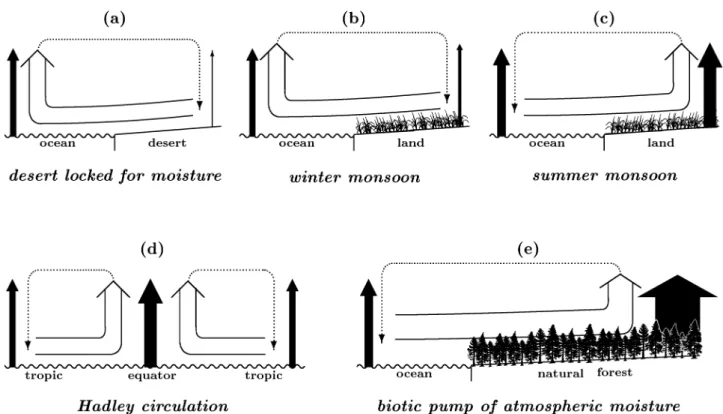
Fig. 4. The physical principle that the low-level air moves from areas with weak evaporation to areas with more intensive evaporation provides clues for the observed patterns of atmospheric circulation. Black arrows: evaporation flux, arrow width schematically indicates the magnitude of this flux (evaporative force). Empty arrows: horizontal and ascending fluxes of moisture-laden air in the lower atmosphere. Dotted arrows: compensating horizontal and descending air fluxes in the upper atmosphere; after condensation of water vapor and precip-itation they are depleted of moisture. (a) Deserts: evaporation on land is close to zero, so the low-level air moves from land to the ocean year round, thus “locking” desert for moisture. (b) Winter monsoon: evaporation from the warmer oceanic surface is larger than evaporation from the colder land surface; the low-level air moves from land to the ocean. (c) Summer monsoon: evaporation from the warmer land surface is larger than evaporation from the colder oceanic surface; the low-level air moves from ocean to land. (d) Hadley circulation (trade winds): evaporation is more intensive on the equator, where the solar flux is larger than in the higher latitudes; low-level air moves towards the equator year round; seasonal displacements of the convergence zone follow the displacement of the area with maximum insolation. (e) Biotic pump of atmospheric moisture: evaporation fluxes regulated by natural forests exceed oceanic evaporation fluxes to the degree when the arising ocean-to-land fluxes of moist air become large enough to compensate losses of water to runoff in the entire river basin year round.

air from the ocean. When the incoming air fluxes ascend, the oceanic moisture condenses and precipitates over the forest. Unburdened of moisture, dry air returns to the ocean from land in the upper atmosphere.

As far as in the natural forest with high leaf area index evaporation, limited by solar radiation only, can exceed evap-oration from the ocean all year round, the corresponding hor-izontal influx of oceanic moisture into the forest can persist throughout the year as well, Fig. 4e. Here lies the difference between the undisturbed natural forest and open ecosystems with low leaf area index. In open ecosystems with low leaf area index the ocean-to-land flux can only originate when the land surface insolation and temperature are higher than on the oceanic surface, Figs. 4b, c.

Total force causing air above the natural forest canopy to ascend is equal to the sum of local evaporative forces gen-erated by local evaporation fluxes of individual trees. On the other hand, this cumulative force acts to pump the

at-mospheric moisture inland from the ocean via the coastline. Therefore, the total flux F (0) of moisture from the ocean to the river basin, which compensates the total runoff, is propor-tional to the number of trees in the forest and, consequently, to the area of the forest-covered river basin. According to the law of matter conservation (continuity equation), the horizontal flux of moisture via the vertical cross-section of the atmospheric column along the coastline, F (0)=WauDh,

where D is the coastline length (basin width), h is the height of moist atmospheric column, u is horizontal air velocity and

Wa(kg H2O m−2) is the moisture content in the atmospheric

column, should be equal to the ascending flux of moisture across the horizontal cross-section of the atmospheric col-umn above the entire river basin of area DL, which is equal to WawfDL, where wfis the vertical velocity of air motion.

From this we obtain wf=uh/L.

The magnitudes of the velocities wf and u are