Nonlinear Feedback Control of VTOL UAVs

HAL Id: hal-01184759

https://hal.archives-ouvertes.fr/hal-01184759

HAL is a multi-disciplinary open access archive for the deposit and dissemination of sci-entific research documents, whether they are pub-lished or not. The documents may come from teaching and research institutions in France or abroad, or from public or private research centers.

L’archive ouverte pluridisciplinaire HAL, est destinée au dépôt et à la diffusion de documents scientifiques de niveau recherche, publiés ou non, émanant des établissements d’enseignement et de recherche français ou étrangers, des laboratoires publics ou privés.

Nonlinear Feedback Control of VTOL UAVs

Daniele Pucci, Minh-Duc Hua, Pascal Morin, Tarek Hamel, Claude Samson

To cite this version:

Daniele Pucci, Minh-Duc Hua, Pascal Morin, Tarek Hamel, Claude Samson. Nonlinear Feedback Control of VTOL UAVs. Aerospace Lab, Alain Appriou, 2014, pp.1-9. �10.12762/2014.AL08-08�. �hal-01184759�

Aerial Robotics

Nonlinear Feedback Control

of VTOL UAVs

T

his paper addresses the nonlinear feedback control of Unmanned Aerial

Vehicles (UAVs) with Vertical Take-Off and Landing (VTOL) capacities, such

as multi-copters, ducted fans, helicopters, convertible UAVs, etc. First, dynamic

models of these systems are recalled and discussed. Then, a nonlinear feedback

control approach is presented. It applies to a large class of VTOL UAVs and aims

at ensuring large stability domains and robustness with respect to unmodeled

dynamics. This approach addresses most control objectives encountered in

practice, for both remotely operated and fully autonomous flight.

Introduction

Like other engineering fields, flight control makes extensive use of linear control techniques [43]. One reason for this is the existence of numerous tools to assess the robustness properties of a linear feedback controller [38] (gain margin, phase margin, H₂, H∞ or LMI techniques, etc.). Another reason is that flight control techniques have been developed primarily for full-size commercial airplanes, which are designed and optimized to fly along very specific trajectories (trim trajectories with a very narrow range of angles of attack). Control design is then typically achieved from the linearized equations of motion along desired trajectories and this makes linear control especially suitable. Some aerial vehicles are required to fly in very diverse conditions, however, with large and rapid variations of the angle of attack. Examples are given by fighter aircraft, convertible aircraft, or small UAVs operating in windy environments. In such cases, ensuring large stability domains matters, and nonlinear feedback designs can be useful for this purpose.

Nonlinear feedback control of aircraft can be traced back to the early eighties. Following [41], control laws based on the dynamic inversion technique have been proposed to extend the flight envelope of military aircraft (see, e.g., [45] and the references therein). The control design strongly relies on tabulated models of aerodynamic forces and moments, like the High-Incidence Research Model (HIRM) of the Group for Aeronautical Research and Technology in Europe (GARTEUR) [26]. Compared to linear techniques, this type of approach allows the flight domain to be extended without involving gain scheduling strategies. The angle of attack is assumed to remain away from the stall zone, however, and should this assumption be violated the behavior of the system is unpredictable. Comparatively, nonlinear feedback control of VTOLs is more recent, but it has been addressed with a larger variety of

techniques. Dynamic inversion has been used as well [10], but many other techniques have also been investigated, such as the Lyapunov-based design [25, 16], Backstepping [4], Sliding modes [4, 46], or Predictive control [20, 3]. A more complete bibliography on this topic can be found in [13]. Most of these studies address the stabilization of hover flight or low-velocity trajectories and therefore little attention is paid to aerodynamic effects. These are typically either ignored or modeled as a simple additive perturbation, the effect of which has to be compensated for by the feedback action. In highly dynamic flight conditions or harsh wind conditions, however, aerodynamic effects become important. This raises several questions, which are little addressed in the control or robotics communities, such as, for example, which models of aerodynamic effects should be considered

for the control design? Or which feedback control solutions can be inferred from these models so as to ensure large stability domains and robustness?

This paper presents a nonlinear feedback control approach for VTOL UAVs, which aims at ensuring large stability domains together with good robustness properties with respect to additive perturbations. The control design covers several control objectives associated with different autonomy levels (teleoperation with thrust direction and thrust intensity reference signals, teleoperation with linear velocity reference signals, fully autonomous flight with position reference signals). The approach, which explicitly takes into account aerodynamic forces in the control design, is particularly well suited to aerial vehicles submitted to small lift forces (e.g., classical multi-copters, or helicopters) or to vehicles with shape symmetry properties with respect to the thrust axis (rockets, missiles, or airplanes with annular wings). The control methodology has been developed by the authors for several years [14, 12, 36, 37] and this paper provides a summary of these developments together with perspectives.

D.Pucci

(Istituto Italiano di Tecnologia) M.-D. Hua, P. Morin (CNRS, UMR 7222) T. Hamel (I3S/UNSA) C. Samson (I3S/UNSA, INRIA) E-mail: daniele.pucci@iit.it DOI : 10.12762/2014.AL08-08

The paper is organized as follows. In § "Dynamics of aircraft motions", dynamical equations of VTOL UAVs are recalled and the various forces affecting the flight dynamics are discussed. § "Preliminaries on control design" provides some preliminaries on the feedback control design and a discussion of the merits of nonlinear feedback control. In § "Symmetric bodies and spherical equivalence", we show that for a class of symmetric bodies, the dynamical equations can be transformed into a simpler form (the so-called "spherical case"). This transformation is then used in § "Control design" to propose a feedback control design method applicable to several vehicles of interest.

Dynamics of aircraft motion

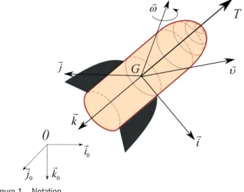
Aircraft dynamics are described by a set of differential equations that characterize the state of the aircraft in terms of the vehicle’s orientation, position, and angular and linear velocities. These variables are measured with respect to some reference frames.

Let =

{

}

  

 denote a fixed inertial frame with respect to (w.r.t.) which the vehicle’s absolute pose is measured. This frame is chosen as the NED frame (North-East-Down) with i0



pointing to the North, j0



pointing to the East, and k₀ pointing to the center of the earth. Let =

{

}

body’s center of mass. The linear and angular velocities v and ω of the body frame  are then defined by

d v OG dt =   _{, d i j k( , , ) ( , , )i j k} dt = ×ω        ₍₁₎

where, here and throughout the paper, the time-derivative is taken w.r.t. the inertial frame I.

T

G

0

k



Equations of motion for a flat earth

Let F and M denote respectively the resultant of the external forces acting on a rigid body of mass m and the moment of these forces

about the body’s center of mass G. Newton’s and Euler’s theorems of

mechanics state that

d p F dt =   _{d h M} dt =   (2) with p mv=  h _{P body}GP (GP ω)dm J.ω ′ ∈ ′ ′ = −

_∫

where J denotes the inertia operator at G. Throughout this paper

aircraft are modeled as rigid bodies of constant mass m and we focus

on the class of vehicles controlled via four control inputs: the thrust intensity T ∈  of a body-fixed thrust force T= −Tk and the three components (in body-frame) of a control torque vector ΓG



. This class of systems contains (modulo an adequate choice of control inputs) most aerial vehicles of interest, like multicopters, helicopters, convertibles UAVs, or even conventional airplanes. The torque actuation can be obtained in different ways, for example, control surfaces (fixed-wing aircraft), propellers (multi-copters), swash-plate mechanism and tail-rotor (helicopters). By neglecting round-earth effects and buoyancy forces1_{, the external forces and moments on the}

aircraft are commonly modeled as follows [8, Ch. 2], [12], [42], [43]:

a b

F = mg + F -Tk + F    

a G

M = GP× F +Tk ×G +G    Θ 

(4)

where g gk= ₀ is the gravity acceleration vector with g the gravity

constant, ( , )F Pa



is the resultant of the aerodynamic forces and its application point2_{, and Θ is the application point of the thrust force.}

In eq. (4) we assume that the gyroscopic torque (usually associated with rotor craft) is negligible or that it has already been compensated via a preliminary torque control action. The force F_b is referred to as a body force. It is induced by the control torque vector Γ_G and thus represents the effect of the control torque actuation on the position dynamics. Conversely, the term Tk G× Θ in (4) represents the effect of the control force actuation on the orientation dynamics.

Besides the gravity force, eq. (4) allows three types of forces (and torques) to be identified:

• body forces, which represent couplings between thrust and torque actuations;

• control forces; • aerodynamic forces.

This decomposition is based on a separation principle that is only valid in first approximation (this issue will be detailed later on). Nevertheless, identifying the dominant effects of dynamics is useful from a control point of view, since it allows generic control strategies to be worked out, which can be refined case by case for specific classes of vehicles. We now discuss the modeling of these three types of forces in more detail. Body forces 2 0 Γ > 1 0 Γ > 3 0 Γ >

L

i



k



Figure 2 – Ducted-fan tail-sitter HoverEye of Bertin Technologies

1_{The aircraft is assumed to be much heavier than air.}

2 _{The point P is the so called body’s center of pressure. This point depends on}

several variables such as the vehicle’s velocity and environmental conditions. As a consequence, its determination is as complex as that of the aerodynamic forces _F_a, and is beyond the scope of this paper.

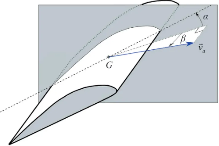
α β G

a

v

Figure 3 – Classic definition of (α, β) angles for a flat wing

The influence of the torque control inputs on the translational dynamics via the body force F_b depends on the torque generation mechanism. More specifically, this coupling term is negligible for quadrotors [9], [32], [6], but it can be significant for helicopters because of the swashplate mechanism [11, Ch.1], [7], [22], [24], [28, Ch. 5] and for ducted-fan tail-sitters because of the rudder system [29, Ch. 3], [31]. Thus, the relevance of this body force must be discussed in relation to the specific application [31] [29, Ch. 3] [13]. Let us remark, however, that the body force F_b is typically small compared to either the gravity, the aerodynamic force, or the thrust force. Similarly, the term Tk G× Θ

in (4), which represents the influence of the thrust control input on the rotational dynamics, is usually small because Θis close to the axis

( , )G k . These body forces will be omitted from now on, since they can be either neglected, or compensated by the control action.

Control forces

The model (4) should be complemented by a modeling of the actuators that generate the inputs T and ΓG



. By assuming that the dynamics of these actuators are (sufficiently) faster than the vehicle’s dynamics, they can be neglected in the first approximation. The effects of the vehicle’s motion and/or wind on the actuation efficiency are another aspect that cannot be neglected if a precise modeling is required. For example, blade flapping is a well-known phenomenon that highlights the difficulty in making the control force and torque completely independent of external aerodynamic conditions for aerial vehicles actuated by propellers. For the sake of simplicity and genericity, we will assume in the paper that it is possible to completely decouple the control action from the vehicle’s motion and wind. We are aware, however, that this can be an important issue in practice.

Aerodynamic forces

The modeling of aerodynamic forces and torques F_a and

a a

M =GP F×  acting on the vehicle remains one of the major problems in the modeling process. Results on this topic can be found in [1] [42, Ch. 2] [43, Ch. 2] for fixed-wing aircraft, in [32] [15] [6] for quadrotors, in [17] [21] [29, Ch. 3] [30] for ducted-fan tail-sitters and in [27], [33], [44] for helicopters. As explained above, we assume that the actuators (e.g., propellers) are not affected by environmental conditions and, therefore, we focus hereafter on the modeling of aerodynamic forces acting on the vehicle’s main body.

A well-accepted general expression of aerodynamic forces and moments can be deduced by applying the so-called Buckingham π theorem [1, p. 34]

[5]. More precisely, we denote with va the air velocity, which is defined as

the difference between v and the wind velocity v_w, i.e., v_a = −v v _w. The lift force F_L is the aerodynamic force component along a perpendicular to the air velocity and the drag force F_D is the aerodynamic force component in the direction of the air velocity. Now, consider a (any) pair of angles (α, β) characterizing the orientation of va with respect to the body frame (e.g.,

figure 3). Combining the Buckingham π−theorem [1, p. 34] with the knowledge

that the intensity of the steady aerodynamic force varies approximately as the square of the air speed | |v_a yields the existence of two dimensionless functions CL(·) and CD(·) depending on the Reynolds number Re, the

Mach number M, and (α, β), and such that

(

)

(

)

where ρ is the free stream air density, Σ is an area germane to the given body shape, r(·) is a unit vector-valued function, and

( )

D

C _{∈ }+ _{and ( )}

L

C ∈  are the aerodynamic characteristics of the body, i.e., the drag coefficient and lift coefficient, respectively. By using the above representation of the aerodynamic force – first introduced in [37] – the lift direction is independent from the aerodynamic coefficients, which in turn characterize the aerodynamic force intensity _{(| | | |}2 2 2₎

a a a L D

F =k v C +C , while the lift direction is fully characterized by the unit vector r(·), which only depends on (α, β) and the air velocity magnitude | |va . We will see that geometric

symmetries of the vehicle’s shape imply precise expressions of the vector r(·).

The main assumption under which the model (5) holds, is that the effects of the vehicle’s rotational and unsteady motions on its surrounding airflow pattern are not preponderant [42, p. 199]. For instance, a constant angular velocity flight generates a different airflow pattern from that in steady cruise, which means that the aerodynamic forces and moments in general depend also on the vehicle’s angular velocity. In addition, the aircraft translational and rotational accelerations also perturb the airflow pattern, which in turn causes transient effects that should be taken into account for precise aerodynamic modeling. These effects will be neglected here, which leads us to assume (5) as the model of the aerodynamic forces.

Preliminaries on control design

From the assumptions and simplifications made in § "Dynamics of aircraft motions", the control model reduces to

a a G ma = mg + F Tk d (i, j,k)= ×(i, j,k) dt d ( J. )= GP×F + dt ω ω − Γ             _    (6) where a dv dt = 

 _{is the linear acceleration of the vehicle. To develop}

general control principles applicable to a large number of aerial vehicles, it is necessary to become free of actuation specificities and

concentrate on the vehicle’s governing dynamics. In agreement with a large number of works on VTOL control (see [13] for a survey) we assume that the torque control Γ_G allows us to modify the body’s instantaneous angular velocity ω at will. Consequently, the angular velocity ω can be considered as an intermediate control input. The above consideration implicitly means that the torque calculation and the ways of producing this torque can be decoupled from high-level control objectives, at least in the first design stage. The corresponding physical assumption is that “almost” any desired angular velocity can be obtained within a short amount of time. In the language of Automatic Control, this is a typical “backstepping” assumption. Once it is made, the vehicle’s actuation consists of four input variables, namely, the thrust intensity and the three components of ω. The control model (6) then reduces to a ma = mg + F Tk d (i, j,k)= ×(i, j,k) dt ω −            (7)

where T and ω are the system’s control inputs. Basics of control design

The control model (7) highlights the role of the gravity force mg and aerodynamic force F_a in obtaining the body’s linear acceleration vector a. It shows, for instance, that to move with a constant reference velocity the controlled thrust vector Tk must be equal to the resultant external force

ext a

F =mg F+ 

When F_a does not depend on the vehicle’s orientation, as in the case of spherical bodies subjected to orientation-independent drag forces only, the resultant external force does not depend on this orientation either (see figure 4 for an illustration). The control strategy then basically consists in aligning the thrust direction k with the direction of F_ext (orientation control with ω) and in opposing the thrust magnitude to the intensity of F_ext (thrust control with T). In

other words, the desired thrust direction and magnitude are defined by

| | | | F k T F F = ± = ±     (8) where ext F F= 

Now, to ensure asymptotic stabilization of the reference velocity, it is necessary to incorporate feedback terms in the velocity dynamics. This can easily be done by changing the definition of F in (8). More precisely, the first equation in (7) can also be written as

( , ) dv ma m F Tk m v t dt ξ = = − +   with a F = mg + F m (v,t)   − ξ  (9)

and where ξ ( , )v t is some stabilizing control, which contains typically both feedback and feedforward terms. It then follows from (8) that

( , )

dv _{v t} dt =ξ

 _

Figure 4 – A physical illustration of the spherical model

When aerodynamic forces depend on the vehicle’s orientation, as is the case of most aerial vehicles, the above control strategy raises important issues. In particular, the resultant force F_ext being now orientation-dependent, the existence and uniqueness of the equilibrium in terms of the vehicle’s orientation is no longer systematic, since the right-hand side of the first equality in (8) may also depend on k. Even when such an equilibrium solution is well defined and locally unique, its stabilization can be very sensitive to thrust orientation variations. As a matter of fact, the capacity of calculating the direction and intensity of F_a at every time-instant – already a quite demanding requirement – is not sufficient to design a control law capable of performing well in (almost) all situations. Knowing how this force changes when the vehicle’s orientation varies is necessary, but is still not sufficient. In the following section we point out the existence of a set of aerodynamic models that allow the control problem to be recast into that of controlling a spherical body. Of course, the underlying assumptions are that these models reflect the physical reality sufficiently well and that the corresponding aerodynamic forces can be either measured or estimated on-line with sufficient accuracy.

Nonlinear versus linear feedback control

Good stability properties can be obtained with linear feedback control for some operating conditions, such as, for example, hover flight with moderate wind, cruising flight at constant or slowly varying linear velocity, etc. In very windy environments or for very aggressive flight, however, several reasons advocate for the use of nonlinear feedback. Let us mention some of them.

• As explained above, the basic principle of aerial vehicle control is to align the thrust direction with the direction of external forces. This orientation control problem can be solved locally, via a local parameterization of the orientation error (e.g., Euler angles). It is well known that this kind of parameterization introduces singularities and artificially limits the stability domain. This is a problem in the case of strong perturbations that can temporarily destabilize the vehicle’s attitude. In order to ensure large stability domains, it is necessary to design the feedback law directly on the underlying manifold (unit sphere for thrust direction control, or special orthogonal group for the control of the full orientation). Linear feedback is not best suited to the control on such compact manifolds.

• From (8), the thrust direction control is well defined only if F does not vanish. This is not a problem around the hover flight configuration, since F F≈ _ext ≈mg. For large initial errors or demanding reference trajectories, however, F may vanish due to the control ξ (see (9)). In

nonlinear one (with norm smaller than the gravity constant), so as to limit the risk of F vanishing.

• Although this problem is not specifically addressed in this paper, control limitations in both magnitude and rate can be problematic in practice. For example, linearizing the model (6) around the hover flight configuration yields two second-order linear systems (yaw and vertical dynamics) and two fourth-order linear systems (horizontal dynamics). While saturating the input of a Hurwitz-stable second-order linear system does not destroy its global asymptotic stability property, this is no longer true for linear systems of higher order (three or more). This also advocates for the use of nonlinear feedback solutions to address these control limitation issues (see for example [2], [18] for results on this topic).

Symmetric bodies and spherical equivalence

We have briefly explained in the previous section the basics of feedback control design for a spherical body (i.e., subjected to aerodynamic forces independent of the vehicle’s orientation). For most vehicles encountered in practice, however, aerodynamic forces depend on the vehicle’s orientation. We show in this section that for a class of such systems, a preliminary feedback transformation on the input allows the dynamics to be rewritten in the same form as in the case of a spherical body. This will be instrumental for the control design methodology described further on.

The expression (5) of the aerodynamic forces holds independently of the body’s shape. As has already been shown in [37], [35], in the case of shape symmetries, aerodynamic properties that simplify the associated control problem can be pointed out.

G

G

k



k



i



i



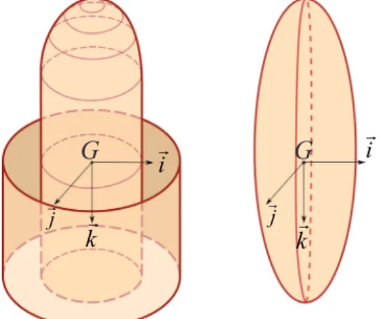
Figure 5 – Symmetric and bisymmetric shapes

α

β

v

G

k



i



Figure 6 – The (α, β) angles

More specifically, if the body’s shape is symmetric3 _{around the thrust}

axis k, then the unit vector r(·) in (5) is given by

cos( ) sin( ) .

r= β − β i ₍₁₀₎

This allows us to decompose the aerodynamic force F_a as follows [37] [35]: | | ( , , ) ( , , )cot( ) ( , , ) | | sin( )

(

)

where α∈[0, ]π is defined as the angle of attack between −k and

a

v , and β∈ −( , ]π π as the angle between the unit frame vector i

and the projection of v_a on the plane

{

}

3 2 1 1 cos atan2( , ) | | a a a a v v v v α ₌ − ₋  β ₌      (12) Note that 1 2 3 | | sin( )cos( ) | | sin( )sin( ) | | cos( ) a a a a a a v v v v v v α β α β α = = = −    (13)

where υa_i

(

)

frame. Note also that the above choice for the angles (α, β) renders the

aerodynamic coefficients in (11) independent of the angle β.

For constant Reynolds and Mach numbers, the aerodynamic coefficients depend only on α. By using the relation (11), it is a simple

matter to establish the following result.

Proposition 1 ([37], [35]) Consider a symmetric thrust-propelled

vehicle. Assume that the aerodynamic forces are given by (5) - (10) and that the aerodynamic coefficients satisfy the following relation

0

( ) ( )cot( )

D L D

C α +C α α =C (14)

where C_D0 denotes a constant number. Then, the body’s dynamic equation (7) can also be written as

p p ma = mg + F T k   −  (15) with 0 2 ( ) | | sin( ) | | L p a a p a D a a C T T k v F k C v v α α = + = −   _{ } (16)

The interest of this proposition is to point out the possibility of viewing a symmetric body subjected to both drag and lift forces as a sphere subjected to the drag force F_p and powered by the thrust force T_p = −T k_p. The main condition is that the relation (14) must be satisfied. Obviously, this condition is compatible with an infinite number of functions C_D and C_L. Let us point out a particular set of simple functions that also satisfy the π-periodicity property with

respect to the angle of attack α associated with bisymmetric bodies. 3 _{See [37], [35] for a precise definition of shape symmetry and bisymmetry.}

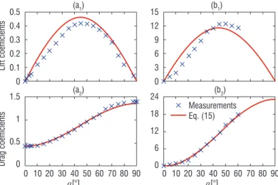
Proposition 2 The functions C_D and C_L defined by 2 0 1 1 ( ) 2 sin ( ), ( ) sin(2 ) D L C c c C c α α α α = + = (17)

where c₀ and c₁ are two real numbers, satisfy the condition (14) with

0 0 21 D

C =c + c . The equivalent drag force and thrust intensity are then given by 0 2 1 | | 2 | | cos( ) p a D a a p a a F k C v v T T c k v α = − = +  _{ }  (18)

A particular bisymmetric body is the sphere whose aerodynamic characteristics (zero lift and constant drag coefficient) are obtained by setting c₁ = 0 in (17). Elliptic-shaped bodies are also symmetric but,

in contrast with the sphere, they do generate lift in addition to drag. The process of approximating measured aerodynamic characteristics with functions given by (17) is illustrated by the figure 7a, where we have used experimental data borrowed from [19, p.19] for an elliptic-shaped body with Mach and Reynolds numbers equal to M = 6 and Re = 7.96 .106 _{respectively. For this example, the identified coefficients}

are c₀ = 0.43 and c₁ = 0.462. Since missile-like devices are “almost”

bisymmetric, approximating their aerodynamic coefficients with such functions can also be attempted. For instance, the approximation shown in figure 7b has been obtained by using experimental data taken from [40, p.54] for a missile moving at M = 0.7. In this case, the identified

coefficients are c₀ = 0.1 and c₁ = 11.55. In both cases, the match

between experimental data and the approximating functions, although far from perfect, should be sufficient for feedback control purposes.

(a1) 0.5 0.4 0.3 0.2 0.1 0 Lif t coefficients (b1) 15 12 9 6 3 0 (a₂) (b₂) Measurements Eq. (15) 0 10 20 30 40 50 60 70 80 90 α[°] 1.5 1 0.5 0 Drag coefficients 0 10 20 30 40 50 60 70 80 90 α[°] 24 18 12 6 0

Figure 7 – Aerodynamic coefficients of: (a_1,2) elliptic bodies; (b_1,2) missile-like bodies

Control design

In this section, we propose nonlinear feedback laws for various control objectives. The first objective is the thrust direction control, which is essential for the control of VTOL UAVs. It is useful by itself, since the basic teleoperation mode for a VTOL UAV relies on thrust direction and thrust intensity reference inputs. Thrust direction control is also the cornerstone for higher-level (semi-)autonomous flight modes, such as, for example, velocity control, position control, or vision-based control. The second objective considered in this section is velocity control. After thrust direction control, velocity control is the next step in increasing the system’s autonomy. Since the velocity dynamics is involved, the role of aerodynamic forces becomes predominant. This will be an opportunity to show the interest of the transformation

proposed in § "Symmetric bodies and spherical equivalence". Once the velocity control level has been defined, the control design can be developed further to address, for example, disturbance rejection and/or position control. These topics are also briefly discussed in this section. Thrust direction control

Consider a time-varying reference thrust (unit) direction k_r. It is assumed that k_r varies smoothly with time, so that dk tr _{( )}

dt



is well defined for any time t. The following result provides control expressions

for the angular velocity control input ω yielding a large stability domain. Proposition 3 The feedback law

0 2 ( · ) (1 · )r r r r k _{k k k k k} k k ω= × +ω − ω +λ +       _{ }   (19) with ω = ×r kr dk_dtr ,k0  

 _{a positive real number, and λ any real number}

(not necessarily constant), ensures exponential stability of the equilibrium k k = _r with domain of attraction { (0) : (0)· (0)k k kr ≠ −1}

  

.

The limitation on the stability domain is related to the topology of the unit sphere, which prevents the existence of smooth autonomous feedback controllers yielding global asymptotic stability. The first term on the right-hand side of (19) is a nonlinear feedback term on the error between k and k_r (here defined from the cross product). The second and third terms are feedforward terms. In practice, these terms are often neglected because the vector dkr

dt



(and thus ω_r) is unknown. For example, if k_r corresponds to a reference thrust direction provided by a pilot via a joystick, dkr

dt



is not available. Omitting these feedforward terms does not prevent good results from being obtained, provided that

0

k is chosen sufficiently large and/or k_r does not vary too rapidly. Finally, the last term on the right-hand side of (19) is associated with the rotation about the axis k (yaw degree of freedom). It does not affect the thrust direction dynamics, since dk k

dt = ×ω

 _  _.

Velocity control for vehicles with symmetric body shapes

Let us thus consider a symmetric vehicle and its velocity dynamics given by (15). The problem is to asymptotically stabilize a reference velocity v_r. We follow the control strategy briefly sketched in § "Preliminaries on control design". Let us define the velocity error

r

v v v  = − and the reference acceleration a_r d _r dtυ =  _{. It follows from} (15) that p r p dv m = F +m(g a ) T k dt − −  _{ }   

The above equation can be written as

( ) p dv m F T k m v dt = − + ξ  _{  }  _ (20)

with

( ( ))

p r

F F=  +m g a − −ξ v (21)

and where ξ( )v is some feedback term. If ξ( )v is chosen as a stabilizing feedback law for the dynamics dv

dt =ξ



 _{, Eq. (20) suggests}

setting Tp =| |F 

and then applying the angular velocity control law of Proposition 3 with k_r defined as the unit vector characterizing the direction of F, i.e., | | r F k F =   

The conditions under which this strategy ensures the asymptotic stability of v = 0 are specified in the following proposition.

Proposition 4 Assume that F does not vanish along the reference trajectory v_r. Then, the feedback law defined by Tp =| |F

 and ω given by (19) with 2 1 ₂ 0 2 ( ) , | | 1 | | v v k k k F v ξ = − = +  _    

k_1,2 two positive real numbers and λ any real number (not necessarily constant), ensures local exponential stability of the equilibrium

( , ) ( , )v k = v kr r

    _.

This proposition is established by showing that the candidate Lyapunov function 2 | | 1 1 (1 · )r V = v + − +α −k k  with 1 2 1 mk k

α > _{, is strictly decreasing along the solutions of the}

controlled system. It is important to note at this point that this property holds true as long as | |F is not zero (so that the control law is well defined). Thus, the limitation on the stability domain only comes from the possibility of F vanishing. Recall from (16) and (21) that

0 | | ( ( ))

a D a a r

F= −k C v v  +m g a − −ξ v

Since ξ( )v is bounded in norm by k₁, it is easy to impose conditions on k₁ and the reference acceleration a_r such that the term

( r ( ))

m g a − −ξ v does not vanish whatever the tracking error v. This is not sufficient to ensure that F never vanishes, however, since the term k Ca D0 | |v va a

 

can take arbitrary values, depending on the value of v. If F does not vanish along the reference trajectory v_r, then local stability is guaranteed and, using the fact that V is decreasing

along the solutions of the controlled system, (possibly conservative) stability domains can be specified.

Note that, in view of (21), the independence of F_p with respect to the vehicle’s orientation in turn implies that F, and thus k_r, are also independent of the vehicle’s orientation. Therefore, the time-derivative of k_r does not depend on the vehicle’s angular velocity ω either and the expression of ω in (19) is well defined. The interest of the invoked transformation, combined with (14), lies precisely there.

In practice, the control law must be complemented with integral correction terms to compensate for almost constant unknown additive

perturbations. With x_r denoting the reference position of the center of mass in the inertial frame, the solution proposed in [12] involves the position error x x x  = − _r expressed in the inertial frame, which is an integral of the velocity error v. To further impose a bound on the integral correction action, a smooth bounded strictly positive function

h defined on [0,+∞) and that satisfies the following properties ([12,

Sec. III.C]) for some positive constant numbers η, μ can be introduced:

2 , | ( ) | s h s s η ∀ ∈_ < and _{0 ( ( ) )h s s}2 s µ ∂ < < ∂

An example of such a function is ( )

1 h s s η = + , with η > 0. It then

suffices to replace the definition of F in (21) by 2

( ( ) (| | ) )

p r

F F=  +m g a − −ξ v +h x x   (22)

with the feedback control law still defined by T_p =| |F and ω given by (19), to obtain a control law that includes an integral correction action and yields strong stability and convergence properties. The above integral correction is, in fact, suited to the case when the control objective of tracking the desired velocity vr is complemented

with that of rendering the position error _{| |x}_ small, with the vehicle’s absolute position x being measured or estimated on-line. Otherwise, it is better to calculate and use a saturated integral of the velocity error. Such an integral _I_v is, for instance, obtained as the (numerical) solution to the following equation [23] [39]

sat (0) 0 v I v I v v I d _{I k I k I} v _I dt k δ  = − +  +  =         (23)

where k_I is a (not necessarily constant) positive number characterizing the desaturation rate, δ > 0 is the upper bound of | |Iv



and satδ _{is the}

classical saturation function defined by sat ( ) min 1, | | x x x δ ₌  δ         . A discrete-time version of this saturated integral is

( ) if | ( ) | ( ) ( ) otherwise | ( ) | v v I j I j I j I j I j  _{∆ ∆ ≤}  ∆ =      (24)

where j ∈ , ∆ is the sampling time period and

( ) (( 1) ) ( )

v v

I j ∆ =I j − ∆ +v j ∆ for j ≥ 1. Setting, for instance,

,0 | | I I v k k δ = +   _{where k}

I,0 > 0, the definition of F

 only has to be replaced by ( ( ) ) p r v v F F=  +m g a − −ξ v +k I (25)

where kυ is a positive gain, to obtain control yielding stability results

similar to those obtained with the previous controllers.

Remark 1 As in the case of velocity control, the position controller

presented previously can also be modified to include an integral action that will improve its convergence properties when slowly varying unmodeled additive terms act on the system. The reader is referred to [12] for complementary details about this modification.

Conclusion and perspectives

This paper has reviewed basic principles of the modeling and control of VTOL UAVs and a nonlinear control approach for a class of vehicles with symmetric body shapes has been proposed. Application examples are given, for example, by rockets and aerial vehicles using annular wings for the production of lift. Specific aerodynamic properties associated with these particular shapes allow for the design of nonlinear feedback controllers yielding asymptotic stability in a very large flight envelope.

Exploiting the aerodynamic characteristics for the design of feedback controllers with large flight envelopes remains a very open research domain. For example, extending the present approach to vehicles with non-symmetric body shapes (e.g., conventional airplanes) is an open topic. A better understanding of the control limitations induced by the stall phenomenon is also necessary (see for example [34] for a study on this topic). Finally, it is very important to take into account the effect of magnitude (and rate) input saturations on the system’s stability n

Acknowledgements

P. Morin has been supported by “Chaire d’excellence en Robotique RTE-UPMC”

References

[1] J.D. ANDERSON – Fundamentals of Aerodynamics. McGraw Hill Series in Aeronautical and Aerospace Engineering, 5th _{edition, 2010.}

[2] J. R. AzINHEIRA and A. MOUTINHO – Hovering Control of an UAv with Backtepping Design Including Input Saturations. IEEE Trans. on Control Systems Technology, 16(3):517–526, 2008.

[3] S. BERTRAND, H. PIET-LAHANIER and T. HAMEL – Contractive Model Predictive Control of an Unmanned Aerial vehicle Model. 17th _{IFAC Symp. on Automatic}

Control in Aerospace, Volume 17, 2007.

[4] S. BOUABDALLAH and R. SIEGWART – Backstepping and Sliding-Mode Techniques Applied to an Indoor Micro Quadrotor. IEEE International Conference on Robotics and Automation, 2005.

[5] P. W. BRIDGMAN – Dimensional Analysis. Encyclopedia Britannica (Wm. Haley, Editor-in-Chief ), 7:439–449, 1969.

[6] P.J. BRISTEAU, P. MARTIN and E. SALAUN – The Role of Propeller Aerodynamics in the Model of a Quadrotor UAv. European Control Conference, pp. 683–688, 2009. [7] A. DzUL, T. HAMEL and R. LOzANO – Modeling and Nonlinear Control for a Coaxial Helicopter. IEEE Conf. on Systems, Man and Cybernetics, Vol. 6, 2002. [8] T. I. FOSSEN – Guidance and Control of Ocean vehicles. John Wiley and Sons, 1994.

[9] T. HAMEL, R. MAHONy, R. LOzANO and J. OSTROWSKI – Dynamic Modelling and Configuration Stabilization for an X4-Flyer. IFAC World Congress, pp. 200–212, 2002. [10] J. HAUSER, S. SASTRy and G. MEyER – Nonlinear Control Design for Slightly Non-Minimum Phase Systems: Application to v/Stol. Automatica, 28:651–670, 1992. [11] M.-D. HUA – Contributions to the Automatic Control of Aerial vehicles. PhD thesis, http://hal.archives-ouvertes.fr/tel-00460801, Université de Nice-Sophia Antipolis, 2009.

[12] M.-D. HUA, T. HAMEL, P. MORIN and C. SAMSON – A Control Approach for Thrust-Propelled Underactuated vehicles and its Application to vTOl Drones. IEEE Trans. on Automatic Control, 54(8):1837–1853, 2009.

[13] M.-D. HUA, T. HAMEL, P. MORIN and C. SAMSON – Introduction to Feedback Control of Underactuated vTOl vehicles. IEEE Control Systems Magazine, pp. 61–75, 2013.

[14] M.-D. HUA, P. MORIN and C. SAMSON – Balanced-Force-Control for Underactuated Thrust-Propelled vehicles. IEEE Conf. on Decision and Control, pp. 6435– 6441, 2007.

[15] H. HUANG, G. M. HOFFMANN, S. L. WASLANDER and C. J. TOMLIN – Aerodynamics and Control of Autonomous Quadrotor Helicopters in Aggressive

Maneuvering. IEEE Conf. on Robotics and Automation, pp. 3277– 3282, 2009.

[16] A. ISIDORI, L. MARCONI and A. SERRANI – Robust Autonomous Guidance: an Internal-Model Based Approach. Springer Verlag, 2003.

[17] E. N. JOHNSON and M. A. TURBE – Modeling, Control and Flight Testing of a Small Ducted Fan Aircraft. Journal of Guidance, Control, and Dynamics, 29(4):769–779, 2006.

[18] F. KENDOUL, D. LARA, I. FANTONI and R. LOzANO – Nonlinear Control for Systems with Bounded Inputs: Real-Time Embedded Control Applied to UAvs. IEEE Conf. on Decision and Control, pp. 5888–5893, 2006.

[19] J. W. KEyES – Aerodynamic Characteristics of lenticular and Elliptic Shaped Configurations at a Mach Number of 6. Technical Report NASA-TN-D-2606, NASA, 1965. [20] H. J. KIM, D. H. SHIM and S. SASTRy – Nonlinear Model Predictive Tracking Control for Rotorcraft-Based Unmanned Aerial vehicles. American Control Conference, pp. 3576–3581, 2002.

[21] A. KO, O. J. OHANIAN and P. GELHAUSEN – Ducted Fan UAv Modeling and Simulation in Preliminary Design. AIAA Modeling and Simulation Technologies Conference and Exhibit, n° 2007–6375, 2007.

[22] T. J. KOO and S. SASTRy – Output Tracking Control Design for a Helicopter Model Based on Approximate linearization. IEEE Conf. on Decision and Control, pp. 3635–3640, 1998.

[23] C. SAMSON and M.-D. HUA – Time Sub-Optimal Nonlinear Pi and Pid Controllers Applied to longitudinal Headway Car Control. Int. J. of Control, 84-10:1717–1728, 2011. [24] R. MAHONy, T. HAMEL and A. DzUL – Hover Control via an Approximate lyapunov Control for a Model Helicopter. IEEE Conf. on Decision and Control, pp. 3490–3495, 1999. [25] L. MARCONI, A. ISIDORI and A. SERRANI – Autonomous vertical landing on an Oscillating Platform: an Internal Model Based Approach. Automatica, 38:21–32, 2002. [26] E. MUIR – Robust Flight Control Design Challenge Problem Formulation and Manual: the High Incidence Research Model (HIRM). Robust Flight Control, A Design Challenge (GARTEUR), Vol. 224 of Lecture Notes in Control and Information Sciences, pp. 419–443, Springer Verlag, 1997.

[27] R. NALDI – Prototyping, Modeling and Control of a Class of vtol Aerial Robots. PhD thesis, University of Bologna, 2008.

[28] R. OLFATI-SABER – Nonlinear Control of Underactuated Mechanical Systems with Application to Robotics and Aerospace vehicles. PhD thesis, Massachusetts Institute of Technology, 2001.

[29] J.-M. PFLIMLIN – Commande d’un minidrone à hélice carénée : de la stabilisation dans le vent à la navigation autonome. PhD thesis, Ecole Doctorale Systèmes de Toulouse, 2006.

[30] J.-M. PFLIMLIN, P. BINETTI, P. SOUèRES, T. HAMEL and D. TROUCHET – Modeling and Attitude Control Analysis of a Ducted-Fan Micro Aerial vehicle. Control Engineering Practice, pp. 209–218, 2010.

[31] J.-M. PFLIMLIN, P. SOUèRES and T. HAMEL – Hovering Flight Stabilization in Wind Gusts for Ducted Fan UAv. IEEE Conf. on Decision and Control, pp. 3491–3496, 2004. [32] P. POUNDS, R. MAHONy and P. CORKE – Modelling and Control of a large Quadrotor Robot. Control Engineering Practice, pp. 691–699, 2010.

[33] R.W. PROUTy – Helicopter Performance, Stability and Control. Krieger, 2005.

[34] D. PUCCI – Flight Dynamics and Control in Relation to Stall. American Control Conf. (ACC), pp. 118–124, 2012.

[35] D. PUCCI – Towards a Unified Approach for the Control of Aerial vehicles. PhD thesis, Université de Nice-Sophia Antipolis and “Sapienza” Universita di Roma, 2013. [36] D. PUCCI, T. HAMEL, P. MORIN and C. SAMSON – Nonlinear Control of PvTOl vehicles Subjected to Drag and lift. IEEE Conf. on Decision and Control (CDC), pp. 6177 – 6183, 2011.

[37] D. PUCCI, T. HAMEL, P. MORIN and C. SAMSON – Modeling for Control of Symmetric Aerial vehicles Subjected to Aerodynamic Forces. arXiv, 2012. [38] C. ROOS, C. DöLL and J.-M. BIANNIC – Flight Control laws: Recent Advances in the Evaluation of their Robustness Properties. Aerospace Lab, Issue 4, 2012. [39] H. KHALIL and S. SESHAGIRI – Robust Output Feedback Regulation of Minimum-Phase Nonlinear Systems Using Conditional Integrators. Automatica, 41:43–54, 2005.

[40] B. F. SAFFEL, M. L. HOWARD and E. N. BROOKS – A Method for Predicting the Static Aerodynamic Characteristics of Typical Missile Configurations for Angles

of Attack to 180 Degrees. Technical Report AD0729009, Department of the navy naval ship research and development center, 1971.

[41] S. N. SINGH and A. SCHy – Output Feedback Nonlinear Decoupled Control Synthesis and Observer Design for Maneuvering Aircraft. International Journal of Control, 31(31):781–806, 1980.

[42] R. F. STENGEL – Flight Dynamics. Princeton University Press, 2004.

[43] B. L. STEVENS and F. L. LEWIS – Aircraft Control and Simulation. Wiley-Interscience, 2nd _{edition, 2003.}

[44] J. C. A. VILCHIS, B. BROGLIATO, A. DzUL and R. LOzANO – Nonlinear Modelling and Control of Helicopters. Automatica, 39:1583–1596, 2003.

[45] Q. WANG and R.F. STENGEL – Robust Nonlinear Flight Control of High-Performance Aircraft. IEEE Transactions on Control Systems Technology, 13(1):15–26, 2005. [46] R. XU and U. OzGUNER – Sliding Mode Control of a Class of Underactuated Systems. Automatica, 44:233–241, 2008.

Daniele Pucci received the bachelor and master degrees in

Control Engineering with highest honors from "Sapienza", University of Rome, in 2007 and 2009, respectively. He received the PhD title in Information and Communication Technologies from University of Nice Sophia Antipolis, and in Control Engineering, from “Sapienza” University of Rome, in 2013. Since then, he is a post-doctoral fellow at the Italian Institute of Technology. His research interests include control of nonlinear systems and its applications to aerial vehicles and robotics.

Minh-Duc Hua graduated from Ecole Polytechnique, France,

in 2006, and received his Ph.D. from the University of Nice-Sophia Antipolis, France, in 2009. He spent two years as a postdoctoral researcher at I3S UNS-CNRS, France. He is currently researcher of the French National Centre for Scientific Research (CNRS) at the ISIR laboratory of the University Pierre and Marie Curie (UPMC), France. His research interests include nonlinear control theory, estimation and teleoperation with applications to autonomous mobile robots such as UAVs and AUVs.

Tarek Hamel is Professor at the University of Nice Sophia

Antipolis since 2003. He conducted his Ph.D. research at the University of Technologie of Compiègne (UTC), France, and received his doctorate degree in Robotics from the UTC in 1996. After two years as a research assistant at the (UTC), he joined the Centre d'Etudes de Mécanique d'Ile de France in

1997 as an associate professor. His research interests include nonlinear control theory, estimation and vision-based control with applications to Unmanned Aerial Vehicles. He is currently Associate Editor for IEEE Transactions on Robotics and for Control Engineering Practice.

Pascal Morin received the Maîtrise degree from Université

Paris-Dauphine in 1990, and the Diplôme d'Ingénieur and Ph.D. degrees from Ecole des Mines de Paris in 1992 and 1996 respectively. He spent one year as a post-doctoral fellow in the Control and Dynamical Systems Department at the California Institute of Technology. He was Chargé de Recherche at INRIA, France, from 1997 to 2011. He is currently in charge of the ``Chaire RTE-UPMC Mini-drones autonomes'' at the ISIR lab of University Pierre et Marie Curie (UPMC) in Paris. His research interests include stabilization and estimation problems for nonlinear systems, and applications to mechanical systems such as nonholonomic vehicles or UAVs.

Claude Samson graduated from the Ecole Supérieure

d'Electricité in 1977, and received his Docteur-Ingénieur and Docteur d'Etat degrees from the University of Rennes, in 1980 and 1983, respectively. He joined INRIA in 1981, where he is presently Directeur de Recherche. His research interests are in control theory and its applications to the control of mechanical systems. Dr. Samson is the coauthor, with M. Leborgne and B. Espiau, of the book Robot Control. The Task-Function Approach (Oxford University Press, 1991).

AUTHORS

Acronyms

GARTEUR (Group for Aeronautical Research and Technology in Europe) HIRM (High-Incidence Research Model)

LMI (Linear Matrix Inequality) NED (North-East-Down) UAV (Unmanned Aerial Vehicle) VTOL (Vertical Take-Off and Landing)