Cache optimizations for stream programs

Cache Optimizations for Stream Programs

by

Janis Sermuliisg

Submitted to the Department of Electrical Engineering and Computer

Science

in partial fulfillment of the requirements for the degree of

Master of Engineering in Computer Science and Engineering

at the

MASSACHUSETTS INSTITUTE OF TECHNOLOGY

May 2005

A

@

Massachusetts Institute of Technology 2005. All rights reserved.

The author hereby grants to M.I.T. permission to reproduce and

distribute publicly paper and electronic copies of this thesis

Author ...

and to grant others the right to do so.

OF TECHNOLOGY

JUL 18 2005

LIBRARIES

Department of Elet&rical Engineering and Computer Science

A

May 6, 2005

Certified by....

Saman Amarasinghe

Associate Professor

Thesis Supervisor

Accepted by ..

Arthur C. Smith

Chairman, Department Committee on Graduate Students

Cache Optimizations for Stream Programs

by

Janis Sermulips

Submitted to the Department of Electrical Engineering and Computer Science on May 6, 2005, in partial fulfillment of the

requirements for the degree of

Master of Engineering in Computer Science and Engineering

Abstract

As processor speeds continue to increase, the memory bottleneck remains a primary impediment to attaining performance. Effective use of the memory hierarchy can result in significant performance gains. This thesis focuses on a set of transforma-tions that either reduce cache-miss rate or reduce the number of memory accesses for the class of streaming applications, which are becoming increasingly prevalent in em-bedded, desktop and high-performance processing. A fully automated optimization algorithm is presented that reduces the memory bottleneck for stream applications developed in the high-level stream programming language StreamIt.

This thesis presents four memory optimizations: 1) cache aware fusion, which combines adjacent program components while respecting instruction and data cache constraints, 2) execution scaling, which judiciously repeats execution of program com-ponents to improve instruction and state locality, 3) scalar replacement, which con-verts certain data buffers into a sequence of scalar variables that can be register allocated, and 4) optimized buffer management, which reduces the overall number of memory accesses issued by the program. The cache aware fusion and execution scaling reduce the instruction and data cache-miss rates and are founded upon a sim-ple and intuitive cache model that quantifies the temporal locality for a sequence of actor executions. The scalar replacement and optimized buffer management reduce the number of memory accesses.

An experimental evaluation of the memory optimizations is presented for three different architectures: StrongARM 1110, Pentium 3 and Itanium 2. Compared to unoptimized StreamIt code, the memory optimizations presented in this thesis yield a 257% speedup on the StrongARM, a 154% speedup on the Pentium 3, and a 152% speedup on Itanium 2. These numbers represent averages over our streaming bench-mark suite. The most impressive speedups are demonstrated on an embedded pro-cessor StrongARM, which has only a single data and a single instruction cache, thus increasing the overall cost of memory operations and cache misses.

Thesis Supervisor: Saman Amarasinghe Title: Associate Professor

Acknowledgments

I would like to thank William Thies and Rodric Rabbah for their guidance throughout

my work that led to this thesis. This thesis is an expanded version of a paper [24]

by the author, William Thies, Rodric Rabbah and Saman Amarasinghe that will

appear in proceedings of ACM SIGPLAN/SIGBED 2005 Conference on Languages, Compilers, and Tools for Embedded Systems. I would also like to thank all members of the StreamIt group. I would like to thank William Thies for his work on filter fusion and loop unrolling in the StreamIt compiler. I would like to thank Jasper Lin for his work on scalar replacement and loop unrolling in the StreamIt compiler. I would also like to thank my advisor, Saman Amarasinghe, for his guidance.

Contents

1 Introduction

13

2 Background

17

2.1.4 Implementation of Cache Optimizations . . . . 21

3 Cache Model

23

3.2 D ata Cache . . . . 28

4 Optimization Algorithm

31

4.1.1 Cache Aware Fusion . . . . 32

4.1.2 Execution Scaling . . . . 35

4.2 Scalar Replacement . . . . 37

4.2.1 Scalar Replacement Example . . . . 37

4.2.2 Implications for the Cache Aware Fusion . . . . 38

4.3 Optimized Buffering of Live Items . . . . 40

4.3.1 M odulation . . . . 41

4.3.2 Copy-Shift . . . . 42

4.3.3 Optimized Copy-Shift . . . . 43

5 Experimental Evaluation 45 5.1 Evaluation of Cache Aware Fusion, Scaling and Scalar Replacement . 47 5.2 Evaluation of Copy-Shift and Modulation . . . . 50

5.3 Evaluation of Peek-Scaling and Cut-Peek . . . . 53

5.4 Comparison to Cache Unaware Full Fusion . . . . 56

5.5 Evaluation of Modified Cache Aware Fusion for Pentium 3 and Itanium 2 58 6 Related Work 61 7 Conclusion 65 7.1 Future W ork . . . . 66

List of Figures

2-1 StreamIt code for an FIR filter . . . . 18

2-2 Hierarchical streams in StreamIt. . . . . 18

2-3 Example pipeline with FIR filter. . . . . 19

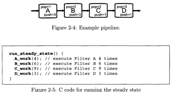
2-4 Example pipeline. . . . . 20

2-5 C code for running the steady state . . . . 20

3-1 Impact of execution scaling on performance. . . . . 27

4-1 Outline of the cache aware fusion algorithm . . . . 34

4-2 Our heuristic for calculating the scaling factor. . . . . 35

4-3 Example StreamIt code . . . . 37

4-4 Generated C code corresponding to the fused filter with no unrolling . 38 4-5 Generated C code corresponding to the fused filter with full unrolling and scalar replacement . . . . 38

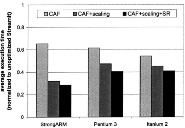
5-1 Impact on average execution time for our benchmark suite. . . . . 47

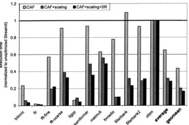
5-2 Performance results for StrongARM 1110 . . . . 49

5-3 Performance results for Pentium 3 . . . . 49

5-4 Performance results for Itanium 2 . . . . 49

5-5 Original StreamIt code for the buffer test. . . . . 51

5-6 Performance of buffer management strategies on a StrongARM 1110 . 52 5-7 Performance of buffer management strategies on a Pentium 3 . . . . . 52

5-8 Performance of buffer management strategies on an Itanium 2 . . . . 52

5-10 Performance of peek-scaling and cut-peek on a Pentium 3 . . . . 55

5-11 Performance of peek-scaling and cut-peek on an Itanium 2 . . . . 55

5-12 Comparison to full fusion on a StrongARM 1110 . . . . 57

5-13 Comparison to full fusion on a Pentium 3 . . . . 57

5-14 Comparison to full fusion on an Itanium 2 . . . . 57

5-15 Performance of cache optimizations after instruction limit modification on a Pentium 3 . . . . 59

5-16 Performance of cache optimizations after instruction limit modification on an Itanium 2 . . . . 59

List of Tables

5.1 Evaluation benchmark suite. . . . . 46

5.2 The best performing buffer management strategies for each

Chapter 1

Introduction

As processor speeds continue to increase, the memory bottleneck remains a primary impediment to attaining performance. Effective use of the memory hierarchy can result in significant performance gains. Current practices for hiding memory latency are invariably expensive and complex. For example, superscalar processors resort to out-of-order execution to hide the latency of cache misses. This results in large power expenditures and also increases the cost of the system. Compilers have also employed computation and data reordering to improve locality, but this requires a heroic analysis due to the obscured parallelism and communication patterns in traditional languages such as C.

For performance-critical programs, the complexity inevitably propagates all the way to the application developer. Programs are written to explicitly manage paral-lelism and to reorder the computation so that the instruction and data working sets fit within the cache. For example, the inputs and outputs of a procedure might be ar-rays that are specifically designed to fit within the data cache on a given architecture; loop bodies are written at a level of granularity that matches the instruction cache. While manual tuning can be effective, the end solutions are not portable. They are also exceedingly difficult to understand, modify, and debug.

The recent emergence of streaming applications presents an opportunity to miti-gate these problems using simple transformations in the compiler. Stream programs are rich with parallelism and regular communication patterns that can be exploited by

the compiler to automatically tune memory performance. Streaming codes encompass a broad spectrum of applications, including embedded communications processing, multimedia encoding and playback, compression, and encryption. They also range to server applications, such as HDTV editing and hyper-spectral imaging. It is natural to express a stream program as a high-level graph of independent components, or

actors. Actors communicate using explicit FIFO channels and can execute whenever

a sufficient number of data items are available on their input channels. In a stream graph, actors can be freely combined and reordered to improve caching behavior as long as there are sufficient inputs to complete each execution. Such transformations can serve to automate tedious approaches that are performed manually using today's languages; they are too complex to perform automatically in hardware or in the most aggressive of C compilers.

1.1

Overview

A naive way to execute a stream program on a uniprocessor is to execute all program components in some precomputed order. However, the size of the instruction footprint of the whole program may not fit into the instruction cache. Thus we need to divide the stream program into parts such that each part has an instruction footprint that fits into the instruction cache; we then scale the execution of the parts to amortize the instruction and data cache misses associated with loading the instructions and state variables associated with each part into the instruction and data cache. The execution scaling needs to be judicious so that the data produced by a scaled stream program part does not exceed the data cache.

This thesis presents four memory optimizations for stream programs: (i) cache aware fusion, (ii) execution scaling, (iii) scalar replacement, and (iv) optimized buffer management. This thesis also presents a simple quantitative model of caching behav-ior for streaming workloads, providing a foundation to reason about the transforma-tions that improve cache usage. Work in this thesis is done in the context of the Synchronous Dataflow [18] model of computation, in which each actor in the stream

graph has a known input and output rate. This is a popular model for a broad range of signal processing and embedded applications.

Cache aware fusion combines adjacent actors into a single function. This allows the compiler to optimize across actor boundaries. The fusion algorithm presented in this thesis is cache aware in that it never fuses a pair of actors that will result in an overflow of the data or the instruction cache. However, our experimental evaluation will show that on some architectures we can relax the instruction cache constraint to

allow more aggressive optimization across actor boundaries.

Execution scaling is a transformation that improves instruction locality by exe-cuting each fused actor in the stream graph multiple times before moving on to the next actor. Since an actor that has been produced using cache aware fusion usually fits within the cache, the repeated executions serve to amortize the cost of loading the actors instruction stream and state from off-chip memory. However, as the cache model will show, actors should not be scaled excessively, as their outputs will eventu-ally overflow the data cache. This thesis presents a simple and effective algorithm for calculating a scaling factor that respects both instruction and data constraints. The cache aware fusion in conjunction with execution scaling represent a unified approach that simultaneously considers the instruction and data working sets.

As actors are fused together, new buffer management strategies become possible. The most aggressive of these, termed scalar replacement, serves to replace an array with a series of local scalar variables. Unlike array references, scalar variables can be register allocated, leading to large performance gains.

We also present several optimized buffer management strategies for FIFO channels that always have to retain a set of live items. We compare two implementations: using a circular buffer, and periodically shifting the live items to the start of the buffer. Our experimental evaluation suggests that shifting the live items is the best implementation if the shifting is performed infrequently.

The memory optimizations presented in this thesis are implemented as part of StreamIt, a language and compiler infrastructure for stream programming [27]. We evaluate the optimizations on three architectures. The StrongARM 1110 represents an

embedded system without a secondary cache, the Pentium 3 represents a superscalar processor and the Itanium 2 represents a VLIW processor. We find that cache aware fusion, scalar replacement, execution scaling and optimized buffer management each offer significant performance gains, and the most consistent speedups result when all are applied together. Compared to unoptimized StreamIt code, the optimizations presented in this thesis yield a 257% speedup on the StrongARM, a 154% speedup on the Pentium 3, and a 152% speedup on Itanium 2. These numbers represent averages over our streaming benchmark suite.

1.2

Organization

This thesis is organized as follows. Chapter 2 gives background information on the StreamIt language. Chapter 3 lays the foundation for the cache optimizations by pre-senting a quantitative model of caching behavior for any sequence of actor executions. Chapter 4 describes cache aware fusion, execution scaling, scalar replacement and op-timized buffer management in detail. Chapter 5 evaluates optimizations proposed in this thesis as they were implemented in the StreamIt compiler. Finally, Chapter 6 describes related work and Chapter 7 concludes the thesis.

Chapter

2

Background

In this chapter we present Streamlt, a high level stream programming language [27].

2.1

Streamlt

StreamIt is an architecture independent language that is designed for stream pro-gramming. In StreamIt, programs are represented as graphs where nodes represent computation and edges represent FIFO-ordered communication of data over tapes. See [27], [10], [28], [17] and [14] for more information and research about Streamlt.

2.1.1

Hierarchical Streams

In Streamlt, the basic programmable unit (i.e., an actor) is a filter. Each filter contains a special function (called work function) that executes atomically, popping (i.e., reading) a fixed number of items from the filter's input tape and pushing (i.e., writing) a fixed number of items to the filter's output tape. A filter may also peek at a given index on its input tape without consuming the item; this makes it simple to represent computation over a sliding window. The push, pop, and peek rates are declared as part of the work function, thereby enabling the compiler to construct a static schedule of filter executions. An example implementation of a Finite Impulse Response (FIR) filter appears in Figure 2-1.

float->float filter FIRFilter (int N, float[] weights) {

// declare work function along with I/O rates work push 1 pop 1 peek N {

float sum = 0;

for (int i = 0; i < N; i++)

// examine items on the input queue

sum += peek(i) * weights[i];

}

pop(); // remove an item from the input queue

push (sum); // enqueue the sum onto the output queue

}

Figure 2-1: StreamIt code for an FIR filter

stream splitter

I joiner

stream

I stream ..-.-.-.- stream stream stream

stream

s _*

stream joiner

(a) pipeline (b) splitjoin (c) feedback loop Figure 2-2: Hierarchical streams in StreamIt.

The work function is invoked (fired) whenever there is sufficient data on the input tape. For the FIR example in Figure 2-1, the filter requires at least N elements before it can execute. The value of N is known at compile time when the filter is constructed. A filter is akin to a class in object oriented programming with the work function serving as the main method. The parameters to a filter (e.g., N and weights) are equivalent to parameters passed to a class constructor.

In StreamIt, the application developer focuses on the hierarchical assembly of the stream graph and its communication topology, rather than on the explicit manage-ment of the data buffers between filters. StreamIt provides three hierarchical struc-tures for composing filters into larger stream graphs (see Figure 2-2). The pipeline construct composes streams in sequence, with the output of one connected to the input of the next. An example of a pipeline appears in Figure 2-3.

Figure 2-3: Example pipeline with FIR filter.

The splitjoin construct distributes data to a set of parallel streams, which are then joined together in a roundrobin fashion. In a splitjoin, the splitter performs the data scattering, and the joiner performs the gathering. A splitter is a specialized filter with a single input and multiple output channels. On every execution step, it can distribute its output to any one of its children in either a duplicate or a roundrobin manner. For the former, incoming data are replicated to every sibling connected to the splitter. For the latter, data are scattered in a roundrobin manner, with each item sent to exactly one child stream, in order. The splitter type and the weights for distributing data to child streams are declared as part of the syntax (e.g., split duplicate or split roundrobin (wi,... , wn)). The splitter counterpart is the joiner. It is a specialized

filter with multiple input channels but only one output channel. The joiner gathers data from its predecessors in a roundrobin manner (declared as part of the syntax) to produce a single output stream.

StreamIt also provides a feedback loop construct for introducing cycles in the graph.

2.1.2

Execution Model

As noted earlier, an actor (i.e., a filter, splitter, or joiner) executes whenever there are enough data items on its input tape. In Streamlt, actors have two epochs of execution: one for initialization, and one for the steady state. The initialization primes the input tapes to allow filters with peeking (i.e. peek rate > pop rate) to execute the very first

instance of their work functions. A steady state is an execution that does not change the buffering in the channels: the number of items on each channel after the execution is the same as it was before the execution. Every valid stream graph has a steady state [18], and within a steady state, there are often many possibilities for interleaving

float -> float pipeline Maino { Source

add Sourceo; // code for Source not shown 4

add FIRO; IFIRi

pOp=1 pop=2 pop=2 pop=3

-e A

B

C

D

-push=3 push=3

H

Figure 2-4: Example pipeline.

runsteady-state() {

A-work(4); // execute Filter A 4 times

B-work(6); / execute Filter B 6 times

C_work(9); // execute Filter C 9 times

D-work(3); / execute Filter D 3 times

}

Figure 2-5: C code for running the steady state

actor executions. An example of a steady state for the pipeline in Figure 2-4 requires filter A to fire 4 times, B 6 times, C 9 times, and D 3 times.

2.1.3

Compilation Process

The StreamIt compiler derives the initialization and steady state schedules [15] and outputs a C program that includes the initialization and work functions, as well as a driver to execute each of the two schedules. The compilation process allows the StreamIt compiler to focus on high level optimizations, and relies on existing compil-ers to perform machine-specific optimizations such as register allocation, instruction scheduling, and code generation-this two-step approach affords us a great deal of portability (e.g., code generated from the StreamIt compiler is compiled and run on

three different machines as reported in Chapter 5).

For example, referring to Figure 2-4, the compiler generates C code for running the steady state that is shown in Figure 2-5.

To execute the program, the steady state is wrapped with another loop that invokes the steady state a designated number of times. Preceding the steady state, a similar initialization schedule is run to prime the data buffers.

2.1.4

Implementation of Cache Optimizations

The cache optimization algorithm presented in this thesis and described in more detail in the Chapter 4 has been implemented in the StreamIt optimizing stream compiler. The cache optimization algorithm first uses cache aware fusion to combine adjacent actors such that each fused actor can fit its instruction and data footprint within the instruction and data cache. The cache optimization algorithm then optimizes fused actors by performing aggressive loop unrolling, scalar replacement, constant propagation and other optimizations supported by the StreamIt compiler. A special compiler pass has been implemented by the author that creates the top level function that invokes the work functions of granularity adjusted actors, scales their execution and implements optimized buffer management strategy.

Chapter 3

Cache Model

From a caching point of view, it is intuitively clear that once an actor's instruction working set is fetched into the cache, we can maximize instruction locality by running the actor as many times as possible. This of course assumes that the total code size for all actors in the steady state exceeds the capacity of the instruction cache. For the benchmarks used in this thesis, the total code size for a steady state ranges from 2 Kb to over 135 Kb (and commonly exceeds 16 Kb). Thus, while individual actors may have a small instruction footprint, the total footprint of the actors in a steady state exceeds a typical instruction cache size. From these observations, it is evident that we must scale the execution of actors in the steady state in order to improve temporal locality. In other words, rather than running a actor n times per steady state, we scale it to run m x n times. We term m the scaling factor.

The obvious question is: to what extent can we scale the execution of actors in the steady state? The answer is non-trivial because scaling, while beneficial to the instruction cache behavior, may overburden the data cache as the buffers between actors may grow to prohibitively large sizes that degrade the data cache behavior. Specifically, if a buffer overflows the cache, then producer-consumer locality is lost.

This chapter presents a simple and intuitive cache model to estimate the instruc-tion and data cache miss rates for a steady state sequence of actor firings. The model serves as a foundation for reasoning about the cache aware optimizations introduced in this thesis. We develop the model first for the instruction cache, and then generalize it to account for the data cache.

3.1

Instruction Cache

A steady state execution is a sequence of actor firings S = (ai, ... , an), and a program

execution corresponds to one or more repetitions of the steady state. We use the

notation S[i] to refer to the actor a that is fired at logical time i, and |S| to denote the length of the sequence.

Our cache model is simple in that it considers each actor in the steady state sequence, and determines whether one or more misses are bound to occur. The miss determination is based on the the instruction reuse distance (IRD), which is equal to the number of unique instructions that are referenced between two executions of the actor under consideration (as they appear in the schedule). The steady state is a compact representation of the whole program execution, and thus, we simply account for the misses within a steady state, and generalize the result to the whole program. Within a steady state, an actor is charged a miss penalty if and only if the number of referenced instructions since the last execution (of the same actor) is greater than the instruction cache capacity.

Formally, let phase(S, i) for 1

<

S:

phase(S, i)

=

(S[i],

S[i

+ 1], ... , S[i + k

-

1])

where k E [1, S] is the smallest integer such that S[i+k] = S[i]. In other words, a

phase is a subsequence of S that starts with the specified actor (S[i]) and ends before the next occurrence of the same actor (i.e., there are no intervening occurrences of S[i] in the phase). Note that because the steady state execution is cyclic, the construction of the subsequence is allowed to wrap around the steady state1. For example, the steady state Si = (AABB) has phase(SI, 1) = (A), phase(S, 2) = (ABB),

phase(Si, 3) = (B), and phase(S1, 4) = (BAA),

'In other words, the subsequence is formed from a new sequence S' = SIS where I represents concatenation.

Let

1(a)

IRD(S, i) =

I(a)

a

where the sum is over all distinct actors a occurring in phase(S, i). We can then determine if a specific actor will result in an instruction cache miss (on its next firing) by evaluating the following step function:

IMISS(Si) = 0 if IRD(S, i) < CI; hit: no cache refill, (3.1) 1 otherwise; miss: (some) cache refill.

In the equation, C represents the instruction cache size.

Using Equation 3.1, we can estimate the instruction miss rate (IMR) of a steady state as:

Isi

IMR(S) = IMISS(S, i). (3.2)

Our cache model allows us to rank the quality of an execution ordering: schedules that boost temporal locality result in miss rates closer to zero, and schedules that do not exploit temporal locality result in miss rates closer to one.

For example, in the steady state Si = (AABB), assume that the combined

instruc-tion working sets exceed the instrucinstruc-tion cache, i.e., I(A) +I (B) > CI. Then, we expect to suffer a miss at the start of every steady state because the phase that precedes the execution of A (at S1[1]) is phase(Si, 2) with an instruction reuse distance greater than the cache size (IRD(Si, 2) >

C).

IMR(Si) = 2/4 whereas for the following variant S2 = (ABAB), IMR(S₂) = 1. In the

case of S2, we know that since the combined instruction working sets of the actors

exceed the cache size, when actor B is fired following A, it evicts part of actor A's instruction working set. Hence when we transition back to fire actor A, we have to

refetch certain instructions, but in the process, we replace parts of actor B's working

set. In terms of the cache model, IRD(S2, i) > C, for every actor in the sequence,

i.e.,

1

1-Note that the amount of refill is proportional to the number of cache lines that are replaced when swapping actors, and as such, we may wish to adjust the cache miss step function (IMISS). One simple variation is to allow for some partial re-placement without unduly penalizing the overall value of the metric. Namely, we can allow the constant Cr to be some fraction greater than the actual cache size. Alterna-tively, we can use a more complicated miss function with a more uniform probability distribution.

Temporal Locality According to our model, the concept of improving temporal instruction locality translates to deriving a steady state where, in the best case, every actor has only one phase that is longer than unit-length. For example, a permutation of the actors in S2 (where all phases are of length two) that improves temporal locality will result in S1, which we have shown has a relatively lower miss rate.

Execution Scaling Another approach to improving temporal locality is to scale the execution of the actors in the steady state. Scaling increases the number of consecutive firings of the same actor. A scaled steady state has a greater number

of unit-length phases (i.e., a phase of length one and the shortest possible reuse distance).

We represent a scaled execution of the steady state as S" = (a ... , a'): the steady state S is scaled by m, which translates to m - 1 additional firings of every actor. For example, scaling S, = (AABB) by a factor of two results in S2 = (AAAABBBB) and scaling S2 = (ABAB) by the same amount results in S22 = (AABBAABB);

From Equation 3.1, we observe that unit-length phases do not increase the in-struction miss rate as long as the size of the actor's inin-struction working set is smaller than the cache size; we assume this is always the case. Therefore, scaling has the effect of preserving the pattern of miss occurrences while also lengthening the steady

14.5 14 13.5 - 13 8 ,S 12.5 E 12 11 10.5 10 0 5 10 15 20 25 30 35 40 scaling factor

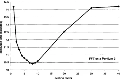
Figure 3-1: Impact of execution scaling on performance.

state. Mathematically, we can substitute into Equation 3.2:

|Stm IMR(Sm) = ]S 1 IMISS(SmIi) 1

Es IMISS(Sm 0.

The last step is possible because IMISS is zero for m - 1 out of m executions of every scaled actor. The result is that the miss rate is inversely proportional to the scaling

factor.

In Figure 3-1 we show a representative curve relating the scaling factor to overall performance. The data corresponds to a coarse-grained implementation of a Fast Fourier Transform (FFT) running on a Pentium 3 architecture. The x-axis represents the scaling factors (with increasing values from left to right). The y-axis represents the execution time and is an indirect indicator of the miss rate (the two measures are positively correlated). The execution time improves in accord with the model: the running time is shortened as the scaling factor grows larger. There is however an

eventual degradation, and as the sequel will show, it is attributed to the data cache performance.

3.2

Data Cache

The results in Figure 3-1 show that scaling can reduce the running time of a program, but ultimately, it degrades performance. This section provides a basic analytical model that helps in reasoning about the relationship between scaling and the data cache miss rate.

We distinguish between two types of data working sets. The static data working set of an actor represents state, e.g., weights in the FIR example (Figure 2-1). The dynamic data working set is the data consumed (poped) from the input channel and generated (pushed) to the output channel by the work function. Both of these working sets impact the data cache behavior of an actor.

Intuitively, the presence of state suggests that it is prudent to maximize that working set's temporal locality. In this case, scaling positively improves the data cache performance. To see that this is true, we can define a data miss rate (DMR) based on a derivation similar to that for the instruction miss rate, replacing C, with

CD _{in Equation 3.1, and 1(a) with State(a) when calculating the reuse distance. Here,}

CD represents the data cache size, and State(a) represents the total size of the static

data in the specified actor.

Execution scaling however also increases the I/O requirements of a scaled actor. Let pop and push denote the declared pop and push rates of an actor, respectively. The scaling of an actor by a factor m therefore increases the pop rate to m x pop and the push rate to m x push. Combined, we represent the dynamic data working set of an actor a as IO(a, m) = m x (pop + push). Therefore, we measure the data reuse

distance (DRD) of an execution S with scaling factor m as follows:

DRD(Sm

, i)

where the sum is over all distinct actors a occurring in phase(Sm, i). While this simple measure double-counts data that are both produced and consumed within a phase, such duplication could be roughly accounted for by using IO'(a, m) = IO(a, m)/2.

We can determine if a specific work function will result in a data cache miss (on its next firing) by evaluating the following step function:

DMISS(S"',

, i) _< CD; hit: no cache refill, (3.4)

1 otherwise; miss: (some) cache refill.

Finally, to model the data miss rate (DMR):

DMR(Sm) = DMISS(S

ISi=Z MS(S1 35

It is evident from Equation 3.5 that scaling can lead to lower data miss rates, as the coefficient 1/Smi = 1/(m x ISI) is inversely proportional to m. However, as

the scaling factor m grows larger, more of the DMISS values transition from 0 to 1 (they increase monotonically with the I/O rate, which is proportional to m). For sufficiently large m, DMR(Sm) = 1. Thus, scaling must be performed in moderation to avoid negatively impacting the data locality.

Note that in order to generalize the data miss rate equation so that it properly accounts for the dynamic working set, we must consider the amount of data reuse within a phase. This is because any actor that fires within phase(Si) might consume some or all of the data generated by S[i]. The current model is simplistic, and leads to exaggerated I/O requirements for a phase. We also do not model the effects of cache conflicts, and take an "atomic" view of cache misses (i.e., either the entire working set hits or misses).

Chapter 4

Optimization Algorithm

In this chapter we describe our memory optimizations that are geared toward im-proving the memory behavior of streaming programs. First, we describe cache aware

fusion which performs a series of granularity adjustments to the actors in the steady

state. The fusion serves to (i) reduce the overhead of switching between actors,

(ii) create coarser grained actors for execution scaling, and (iii) enable novel buffer

management techniques between fused actors. Second, we describe execution

scal-ing which scales a steady state to improve instruction locality, subject to the data

working set constraints of the actors in the stream graph. Third, we describe scalar replacement which enables register allocation of intermediate values that are passed between fused filters. Last, we discuss an optimized management strategy for the data in the FIFO channels to support peeking, that reduce the number of memory accesses without introducing substantial computational overhead.

4.1

Cache Optimizations

The cache aware fusion in conjunction with execution scaling represent a unified cache

optimization that simultaneously considers the instruction and data working sets of

actors that make up a stream program.

4.1.1

Cache Aware Fusion

In StreamIt, the granularity of actors is determined by the application developer, according to the most natural representation of an algorithm. When compiling to a cache-based architecture, the presence of a large number of actors exacerbates the transition overhead between work functions. It is the role of the compiler to adjust the granularity of the stream graph to mitigate the execution overhead.

In this section we describe an actor coarsening technique we refer to as cache

aware

fusion

function is equivalent to its constituents. For example, let an actor A fire n times, and an actor B fire 2n times per steady state: S' = (A"B"B"). Fusing A and B results in an actor F that is equivalent to one firing of A and two firings of B; F fires n times per steady state (Sn = (Fn)). In other terms, the work function for actor F inlines the work functions of A and B.

When two actors are fused, their executions are scaled such that the output rate of one actor matches the input rate of the next. In the example, A and B represent a producer-consumer pair of filters within a pipeline, with filter A pushing two items per firing, and B popping one item per firing. The fusion implicitly scales the execution of B so that it runs twice for every firing of A.

Fusion also reduces the overhead of switching between work functions. In our infrastructure, the steady state is a loop that invokes the work functions via method calls. Thus, every pair of fused actors eliminates a method call (per invocation of the actors). The impact on performance can be significant, but not only because method calls are removed: the fusion of two actors also enables the compiler to optimize across actor boundaries. In particular, for actors that exchange only a few data items, the

compiler can allocate the data streams to registers. The data channel between fused actors is subject to special buffer management techniques (e.g. scalar replacement) as described in the Section 4.2.

There are, however, downsides to fusion. First, as more and more actors are fused, the instruction footprint can dramatically increase, possibly leading to poor use of the instruction cache. Second, fusion increases the data footprint when the fused actors maintain state (e.g., coefficient arrays and lookup tables). Our fusion algorithm is cache aware in that it is cognizant of the instruction and data sizes.

The CAF algorithm uses a greedy fusion heuristic to determine which filters should be fused. It continuously fuses actors until the addition of a new actor causes the fused actor to exceed either the instruction cache capacity, or a fraction of the data cache capacity. For the former, we estimate the instruction code size using a simple count of the number of operations in the intermediate representation of the work function. For the latter, we allow the state of the new fused actor to occupy up to some fraction of the data cache capacity (e.g. 50%).

The algorithm illustrated in Figure 4-1 leverages the hierarchical nature of the stream graph, starting at the leaf nodes and working upward. For pipeline streams, the algorithm identifies the connection in the pipeline with the highest steady-state I/O rate, i.e., the pair of filters that communicate the largest number of items per steady state. These two filters are fused, if doing so respects the instruction and data cache constraints. To prevent fragmentation of the pipeline, each fused filter is further fused with its upstream and downstream neighbors so long as the constraints are met. The algorithm then repeats this process with the next highest-bandwidth connection in the pipeline, continuing until no more filters can be fused. For splitjoin streams, the CAF algorithm fuses all parallel branches together if the combination satisfies the instruction and data constraints. Partial fusion of a splitjoin is not helpful, as the child streams do not communicate directly with each other; however, complete fusion can enable further fusion in parent pipelines.

//

Following recursive algorithm can be used to find a set of

//

partitions for each pipeline or splitjoin such that all actors

//

within a partition can be fused without violating instruction or

//

data cache constraint.

//

For each partition that is returned for the top level pipeline

//

all actors within that partition are fused into a new actor.

//

To find partitions for a pipeline:

Calculate the number of partitions required for each child, if for any child this is > 1 then remember those partitions.

For each sequence (i..J) of children where for each child

number of partitions is 1 use function Interval(ij) to find partitions.

Interval(ij)

"

Find maximum bandwidth connection between children (in the interval (i..j)), let this be a pair m and m + 1.

Estimate instruction and data footprint of fused m and m + 1.

If fused m and m + 1 violates any cache constraint, use Interval(i,m) and Interval(m + 1,j) to find two sets of partitions.

If fused m and m + 1 do not violate any cache constraint, start with

m and m + 1 fused, try fusing up or down until can not fuse up or down

without violating a cache constraint. Let this result in a partition (a..b), use Interval(i,a - 1) and Interval(b + 1,j) to find remaining partitions."

//

To find partitions for a splitjoin:

Calculate the number of partitions required for each child.

If each child can be fused into a single partition, estimate instruction and

data footprint of a fused splitjoin, if this does not violate any cache constraint return a single partition.

Otherwise, return the set of partitions required for each child. Figure 4-1: Outline of the cache aware fusion algorithm

//

//

//

//

//

{

create array M of size ISI

for i = 1 to |SI

{

//

c' = a x (c - State(a))

//

//

M[i] = round(c' / 1O(a, 1))

}

sort M into ascending numerical order

i = [ (1 -p) x IS1

J

return M[i]

}

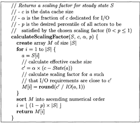
Figure 4-2: Our heuristic for calculating the scaling factor.

4.1.2

Execution Scaling

After we have applied the cache aware fusion algorithm the next step is to scale the granularity adjusted actors in order to reduce the cache-miss rate. According to our instruction cache model, increasing the number of consecutive firings of the same actor leads to lower instruction cache miss rates. However, scaling increases the data buffers that are maintained between actors. Thus it is prudent that we account for the data working set requirements as we scale a steady state.

Our approach is to scale the entire steady state by a single scaling factor, with the constraint that only a small percentage of the actors are allowed to overflow the data cache. Our two-staged algorithm is outlined in Figure 4-2.

First, the algorithm calculates the largest possible scaling factor for every actor that appears in the steady state. To do this, it calculates the amount of data consumed and produced by each actor firing and divides the available data cache size by this data production rate. In addition, the algorithm can toggle the effective cache size to account for various eviction policies.

Second, it chooses the largest factor that allows a fraction p of the steady state actors to be scaled safely (i.e., the cache is adequate for their I/O requirements). For example, the algorithm might calculate mA = 10, mB = 20, mc = 30, and mD = 40, for four actors in some steady state. That is, scaling actor A beyond 10 consecutive iterations will cause its dynamic I/O requirements to exceed the data cache. Therefore, the largest m that allows p = 90% of the actors to be scaled

without violating the cache constraints is 10. Similarly, to allow for the safe scaling of p = 75% of the actors, the largest factor we can choose is 20.

In our implementation, we use a 90-10 heuristic. In other words, we set p = 90%.

We empirically determined this value via a series of experiments using our benchmark suite. See Appendix A for an experimental evaluation of our heuristic.

Note that our algorithm adjusts the effective cache size that is reserved for an actor's dynamic working set (i.e., data accessed via pop and push). This adjustment allows us to control the fraction of the cache that is used for reading and writing data-and affords some flexibility in targeting various cache organizations. For ex-ample, architectures with highly associative and multilevel caches may benefit from scaling up the effective cache size (i.e., a > 1), whereas a direct mapped cache that is more prone to conflicts may benefit from scaling down the cache (i.e., a < 1). In our

implementation, we found a = 2/3 to work well on desktop processors Pentium 3 and

Itanium 2, and a = 4/3 to work well on an embedded processor StrongARM 1110. We note that the optimal choice for the effective cache size is a complex function of the underlying cache organization and possibly the application as well; this is an interesting issue that warrants further investigation.

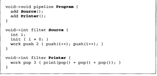
Figure 4-3: Example StreamIt code

4.2

Scalar Replacement

After two filters have been fused into a single work function using cache aware fusion, the buffer that contains the intermediate values can be replaced by a set of scalar variables. Such transformation allows the C compiler to register allocate intermediate values and it also eliminates the need to keep track of the current index within the buffer while adding to or removing items from the buffer. In order for the scalar

replacement to be possible all instructions that access the buffer must access it with

a constant index. As our example will show, we can guarantee this property by performing sufficient loop unrolling.

4.2.1

Scalar Replacement Example

Consider a StreamIt program shown in Figure 4-3. The program consists of two filters (Source and Printer) that have mis-matched rates (filter Source pushes two items and filter Printer pops three items). If the two filters are fused the compiler will create a pair of loops to match the production and consumption rates as shown in the Figure 4-4. Note that we can not replace the buffer with scalar variables yet since each instruction that accesses the buffer uses a non-constant subscript. To allow

scalar replacement we need to fully unroll the loops. Note that the result will have

three copies of instructions that correspond to the filter Source and two copies of

void->void pipeline Program { add Source);

add Printer(;

I

void->int filter Source { int i;

init { i = 0;

work push 2 { push(i++); push(i++); }

I

void->int filter Printer {

work pop 3 { print(pop() + pop() + pop(); I

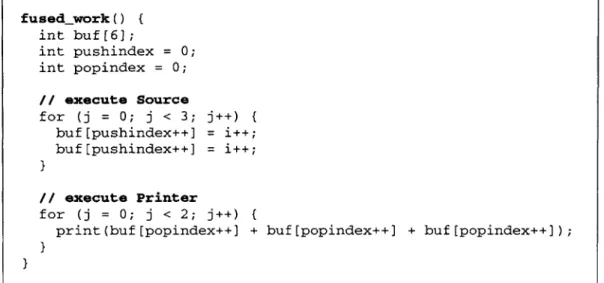
fused work() int buf[6]; int pushindex = 0; int popindex = 0; // execute Source for (j = 0; j < 3; j++) { buf[pushindex++] = i++; buf[pushindex++] = i++; } // execute Printer for (j = 0; j < 2; j++)

print(buf[popindex++] + buf[popindex++] + buf[popindex++]);

}

}

Figure 4-4: Generated C code corresponding to the fused filter with no unrolling

fusedwork() {

int bufO, buf1, buf2, buf3, buf4, buf5;

buf0 = i++; bufl = i++; // execute Source

buf2 = i++; buf3 = i++; // execute Source

buf4 = i++; buf5 = i++; // execute Source

print(buf0 + buf1 + buf2); // execute Printer

print(buf3 + buf4 + buf5); // execute Printer

}

Figure 4-5: Generated C code corresponding to the fused filter with full unrolling and scalar replacement

instructions that correspond to the filter Printer. Figure 4-5 shows the C code that has been generated after StreamIt compiler has performed full loop unrolling and

scalar replacement.

4.2.2

Implications for the Cache Aware Fusion

The goal of fusion is to allow aggressive optimization across actor boundaries. Our cache aware fusion algorithm is modified to only fuse a group of filters if a given unroll limit will allow all intermediate buffers to be scalar replaced. For our StreamIt example in Figure 4-3 the filters Source and Printer will only be fused if the loop unrolling limit is greater than or equal to 3 (otherwise the loop around the statements

corresponding to filter Source in the fused work function will not be fully unrolled). For our benchmark suite we use an unrolling limit of 128 to allow as much fusion and scalar replacement as possible. The cache aware fusion algorithm also keeps track of the code size expansion due to loop unrolling, so that the instruction size of the new actor after unrolling does not exceed the instruction cache.

4.2.3

Implications for Unrolling

We need to perform aggressive unrolling to maximize the number of buffers that are replaced by scalars. However, not all loops should be fully unrolled. For example fully unrolling a loop that does not perform any push or pop operations unnecessarily increases the instruction size of the actor (this may limit our ability to fuse an actor with other actors without exceeding the instruction cache). Therefore loops that do not perform push or pop operations are unrolled no more than 4 times.

4.3

Optimized Buffering of Live Items

For FIFO channels where the consumer only examines (peeks) the same items that it consumes during each iteration (peek < pop) a simple buffer of sufficient size can be used. The buffer is first filled up by the producer and subsequently emptied by the consumer. As shown in the previous section such buffers can be replaced with a set of scalar variables if the two filters are fused and sufficient loop unrolling is performed.

For FIFO channels where the consumer examines more items than it consumes

(peek > pop) the buffer will be primed during the initialization phase to allow the

consumer to execute. Subsequently, the buffer is never completely emptied by the consumer. This imposes a difficult decision on our StreamIt compiler of how to best implement a buffer that has to retain a set of live items for consumption during subsequent steady state cycles.

We explore two basic strategies for implementing buffers that must retain live items between steady state executions. The first strategy, termed modulation, im-plements a traditional circular buffer that is indexed via a wrap-around head and tail pointers. The second strategy, termed copy-shift, avoids modulo operations by shifting the buffer contents to the start of the buffer after a certain number of execu-tions. Our experimental evaluation demonstrates that, while a naive implementation of copy-shift can be 2x to 3x slower than modulation, optimizations that utilize execution scaling can boost the performance of copy-shift to be significantly faster than modulation (51% speedup on StrongARM, 48% speedup on Pentium 3, and 5% speedup on Itanium 2).

4.3.1

Modulation

The modulation scheme uses a traditional circular-buffer approach. Three vari-ables are introduced: a BUFFER to hold all items transferred between the actors, a push-index to indicate the buffer location that will be written next, and a pop-index to indicate the buffer location that will be read next (i.e., the location corresponding to peek(O)). The communication primitives are translated as follows:

push(val); ==> BUFFER[push-index] := val;

push-index := (pushindex + 1) % BUF_SIZE;

pop(); := BUFFER[pop-index];

pop-index := (pop-index + 1) % BUFSIZE;

peek(i) := BUFFER[(pop-index + i) % BUFSIZE]

Note that, for performance reasons the StreamIt compiler converts the modulo oper-ations to bitwise-and operoper-ations by scaling the buffer to a power of two.

4.3.2

Copy-Shift

A copy-shift implementation allows us to eliminate the bitwise-and operations, by

not allowing the head and tail pointers to wrap around the buffer. Instead, the live items are periodically copied to the start of the buffer and the head and tail pointers are decreased. The communication primitives are translated as follows:

push(val); ==> BUFFER[push index++] := val;

pop(); := BUFFER[popjindex++];

peek(i) := BUFFER[pop-index + i]

An unoptimized implementation of copy-shift in our StreamIt compiler copies the live items after each execution of the consumer that has been scaled only to match rates with other fused actors. The cost of copying a substantial amount of data frequently makes the unoptimized copy-shift substantially less efficient than simple modulation as our experimental evaluation will show.

4.3.3

Optimized Copy-Shift

We can reduce the cost of copy-shift by increasing the size of the data buffer. This allows us to reduce the frequency at which the live items are copied over to the beginning of the buffer. We evaluate two transformations of a stream program that allow us to reduce the frequency of copying the live items.

Peek-Scaling Implementation

A simple transformation, that allows us to reduce the number of times the live items

are copied, is to replace every filter that peeks (i.e., peek > pop) with a filter that executes the original filter N times. N is chosen sufficiently large such that the cost of copying items per execution of the original filter is reduced (since live items will be copied to the beginning of the buffer N times less). After scaling, the new

filter has a pop rate equal to pop, = N * popo and a peek rate equal to peek, =

N * popo + (peeko - popo), where popo and peek, are the pop and peek rates of the

original filter, and pop, and peek, are the pop and peek rates of the replaced filter.

The compiler choses N such that (peek, - pop.) <; popn/4 (the original filter is

executed N times such that the new filter consumes at least 4x as many items than are copied over to the start of buffer after every iteration of the new filter). As our experimental evaluation will show this transformation allows copy-shift to outperform modulation for our synthetic benchmark. However, this transformation can lead to significant performance reduction for some of our application benchmarks, since the loop that is introduced by the peek-scaling will be unrolled to allow scalar replacement leading to an increase in the instruction footprint. Also the loops enclosing other fused actors will have larger iteration counts to match the new consumption/production rate of the replaced filter; this leads to increased code size due to unrolling. Lastly, the sum of input and output data consumed during a steady state for some actor after the peek-scaling transformation might exceed the size of the data cache leading to bad data cache performance.

Cut-Peek Implementation

Another approach that allows us to decrease the frequency at which live items are copied to the start of the buffer is to modify our cache aware fusion algorithm to never fuse a producer consumer pair if the consumer performs any peeking (i.e., peek > pop).

This ensures that after we perform execution scaling we can copy the live items only once per execution of the scaled consumer (which might be fused with filters that consume its output). The cut-peek implementation presents a unified optimization framework for reducing cache miss rates and achieving good performance for our copy-shift buffer implementation.

Chapter 5

Experimental Evaluation

In this chapter we evaluate the merits of the proposed memory optimizations and buffer management strategies. We use three different architectures: a 137 MHz

Stron-gARM 1110, a 600 MHz Pentium 3 and a 1.3 GHz Itanium 2. The StronStron-gARM results

reflect performance for an embedded target; it has a 16 Kb Li instruction cache, an 8 Kb Li data cache, and no L2 cache. The StrongARM also has a separate 512-byte minicache (not targeted by our optimizations). The Pentium 3 and Itanium 2 reflect desktop performance; they have a 16 Kb Li instruction cache, 16 Kb Li data cache,

and 256 Kb shared L2 cache.

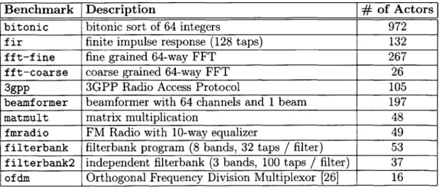
Our benchmark suite (see Table 5.1) consists of 11 StreamIt applications. They are compiled with the StreamIt compiler which applies the optimizations described in this thesis, as well as aggressive loop unrolling (by a factor of 128 for all benchmarks) to facilitate scalar replacement (see Chapter 4). The StreamIt compiler outputs a functionally equivalent C program that is compiled with gcc (v3.4, -03) for the StrongARM and for the Pentium 3, and with ecc (v7.0, -03) for the Itanium 2. Each benchmark is then run five times, and the median user time is recorded.

As the StrongARM does not have a floating point unit, we converted all of our floating point applications (i.e., every application except for bitonic) to operate on integers rather than floats. In practice, a detailed precision analysis is needed in converting such applications to fixed-point. However, as the control flow within these applications is very static, we are able to preserve the computation pattern for the

Benchmark Description

#

of Actors

bitonic bitonic sort of 64 integers 972

f ir finite impulse response (128 taps) 132

f f t-f ine fine grained 64-way FFT 267

fft-coarse coarse grained 64-way FFT 26

3gpp 3GPP Radio Access Protocol 105

beamf ormer beamformer with 64 channels and 1 beam 197

matmult matrix multiplication 48

fmradio FM Radio with 10-way equalizer 49

filterbank filterbank program (8 bands, 32 taps

/

filterbank2 independent filterbank (3 bands, 100 taps

/

of dm Orthogonal Frequency Division Multiplexor [26] 16

Table 5.1: Evaluation benchmark suite.

sake of benchmarking by simply replacing every floating point type with an integer type.

We also made an additional modification in compiling to the StrongARM: our execution scaling heuristic scales actors until their output fills 4/3 of the data cache, rather than 2/3 used for the Pentium 3 and the Itanium 2. This modification accounts for the 32-way set-associative Li data cache in the StrongARM. Due to the high degree of associativity, there is a smaller chance that the actor outputs will repeatedly evict the state variables of the actor, thereby making it worthwhile to further fill the data cache. Note, that, since 4/3 > 1, we expect the data produced by the actor to overwrite the data consumed without evicting the state. Using 4/3 instead of 2/3 on StrongARM yields up to 30% improvement on some benchmarks.