Certifiably correct SLAM

(1)

Certifiably Correct SLAM

by

David M. Rosen

B.S., California Institute of Technology (2008)

M.A., The University of Texas at Austin (2010)

Submitted to the Department of Electrical Engineering and Computer

Science

in partial fulfillment of the requirements for the degree of

Doctor of Science

at the

MASSACHUSETTS INSTITUTE OF TECHNOLOGY

September 2016

c

○ David M. Rosen, MMXVI. All rights reserved.

The author hereby grants to MIT permission to reproduce and to

distribute publicly paper and electronic copies of this thesis document

in whole or in part in any medium now known or hereafter created.

Author . . . .

Department of Electrical Engineering and Computer Science

August 31, 2016

Certified by. . . .

Professor John J. Leonard

Samuel C. Collins Professor of Mechanical and Ocean Engineering

Thesis Supervisor

Accepted by . . . .

Professor Leslie A. Kolodziejski

Chair, EECS Committee on Graduate Students

(2)

(3)

Certifiably Correct SLAM

by

David M. Rosen

Submitted to the Department of Electrical Engineering and Computer Science on August 31, 2016, in partial fulfillment of the

requirements for the degree of Doctor of Science

Abstract

The ability to construct an accurate model of the environment is an essential capabil-ity for mobile autonomous systems, enabling such fundamental functions as planning, navigation, and manipulation. However, the general form of this problem, simul-taneous localization and mapping (SLAM), is typically formulated as a maximum-likelihood estimation (MLE) that requires solving a nonconvex nonlinear program, which is computationally hard. Current state-of-the-art SLAM algorithms address this difficulty by applying fast local optimization methods to compute a critical point of the MLE. While this approach has enabled significant advances in SLAM as a practical technology by admitting the development of fast and scalable estimation methods, it provides no guarantees on the quality of the recovered estimates. This lack of reliability in existing SLAM algorithms in turn presents a serious barrier to the development of robust autonomous systems generally.

To address this problem, in this thesis we develop a suite of algorithms for SLAM that preserve the computational efficiency of existing state-of-the-art methods while additionally providing explicit performance guarantees. Our contribution is threefold. First, we develop a provably reliable method for performing fast local optimization in the online setting. Our algorithm, Robust Incremental least-Squares Estimation (RISE), maintains the superlinear convergence rate of existing state-of-the-art online SLAM solvers while providing superior robustness to nonlinearity and numerical ill-conditioning; in particular, we prove that RISE is globally convergent under very mild hypotheses (namely, that the objective is twice-continuously differentiable with bounded sublevel sets). We show experimentally that RISE’s enhanced convergence properties lead to dramatically improved performance versus alternative methods on SLAM problems exhibiting strong nonlinearities, such as those encountered in visual mapping or when employing robust cost functions.

Next, we address the lack of a priori performance guarantees when applying local optimization methods to the nonconvex SLAM MLE by proposing a post hoc verifica-tion method for computaverifica-tionally certifying the correctness of a recovered estimate for pose-graph SLAM. The crux of our approach is the development of a (convex) semidef-inite relaxation of the SLAM MLE that is frequently exact in the low to moderate

(4)

measurement noise regime. We show that when exactness holds, it is straightforward to construct an optimal solution 𝑍* _{for this relaxation from an optimal solution 𝑥}* _of

the SLAM problem; the dual solution 𝑍* _{(whose optimality can be verified directly}

post hoc) then serves as a certificate of optimality for the solution 𝑥* _{from which}

it was constructed. Extensive evaluation on a variety of simulated and real-world pose-graph SLAM datasets shows that this verification method succeeds in certifying optimal solutions across a broad spectrum of operating conditions, including those typically encountered in application.

Our final contribution is the development of SE-Sync, a pose-graph SLAM in-ference algorithm that employs a fast purpose-built optimization method to directly solve the aforementioned semidefinite relaxation, and thereby recover a certifiably globally optimal solution of the SLAM MLE whenever exactness holds. As in the case of our verification technique, extensive empirical evaluation on a variety of simulated and real-world datasets shows that SE-Sync is capable of recovering globally optimal pose-graph SLAM solutions across a broad spectrum of operating conditions (includ-ing those typically encountered in application), and does so at a computational cost that scales comparably with that of fast Newton-based local search techniques.

Collectively, these algorithms provide fast and robust inference and verification methods for pose-graph SLAM in both the online and offline settings, and can be straightforwardly incorporated into existing concurrent filtering smoothing architec-tures. The result is a framework for real-time mapping and navigation that preserves the computational speed of current state-of-the-art techniques while delivering certi-fiably correct solutions.

Thesis Supervisor: Professor John J. Leonard

(5)

Acknowledgments

While there may only be one author listed on the title page of this document, the production of a doctoral thesis, like most scientific endeavors, is a team effort, and I am deeply grateful to the many friends and colleagues who have contributed to the success of this enterprise.

First and foremost, I would like to thank my doctoral advisor John Leonard for enabling me to come to MIT, and for his unwavering and enthusiastic support of my research program, especially for those projects in which the approach was unortho-dox and the outcome far from certain at the outset. Having the freedom to pursue investigations wherever they lead at an institution as intellectually vibrant as MIT has been a truly superlative experience.

I have also been privileged to collaborate with an extraordinarily talented and generous group of postdoctoral scholars and research scientists over the course of my graduate studies. I am particularly indebted to Michael Kaess, whose work on online mapping methods inspired me to seek out the Marine Robotics Group at CSAIL, and who very graciously supported my rooting around in the codebase for his signature algorithms as part of my first real research project as a graduate student.1 _{I have}

likewise been extraordinarily fortunate to collaborate with Luca Carlone and Afonso Bandeira on the development of the semidefinite relaxation methods for pose-graph SLAM that form the second half of this thesis; if I could have drafted my own fantasy team of researchers for this project, I would have picked them, and working alongside them on it has been an absolute joy.

I would also like to thank the other members and affiliates of the Marine Robotics Group for being such wonderful colleagues. Special thanks to Maurice Fallon, Liam Paull, Andrea Censi, Michael Novitzky, Mark van Middlesworth, Ross Finman, De-hann Fourie, Sudeep Pillai, Janille Maragh, Julian Straub, Pedro Teixeira, and Mei Cheung for putting up with me for as long as they have. Their good humor and willingness to engage in regular “vigorous intellectual exercise” have made going to

(6)

work (and particularly conferences) both edifying and tremendously fun.

Aside from work, I am beyond grateful for the many friends both here in Cam-bridge and around the world that have made this six-year period the wonderful ex-perience that it has been; this has truly been an embarrassment of riches far beyond what could properly be accounted here. Special thanks to the extended Sidney-Pacific Graduate Community (particularly Ahmed Helal, Burcu Erkmen, Jit Hin Tan, Matt and Amanda Edwards, George Chen, Boris Braverman, Dina El-Zanfaly, Rachael Harding, Fabián Kozynski, Jenny Wang, Brian Spatocco, and Tarun Jain) for mak-ing MIT feel like home, to the extended Lloyd House alumni (particularly Kevin Watts and Melinda Jenkins, Tim and Chelsea Curran, Joe Donovan, Vamsi Chavakula and Christina Weng, Vivek and Karthik Narsimhan, Matt Lew, Hanwen Yan, Chi Wan Ko, and Stephen Cheng) for friendship that has spanned decades(!) and continents, and to Christina Zimmermann for her patience, support, and good humor during the final hectic sprint to complete my defense and this document.

And finally, tremendous thanks to my family for their enduring patience and support throughout my time at MIT. Special thanks to my mom, who has been the recipient of more than her fair share of odd-hours dark-night-of-the-soul phone calls during the more difficult periods of this research (years 4–5),2 _{and to my grandfather}

Arthur Adam, for showing me the pleasure of finding things out. Without them, none of this would have been possible.

(7)

List of Figures

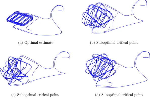
1-1 Examples of suboptimal estimates in pose-graph SLAM . . . 19

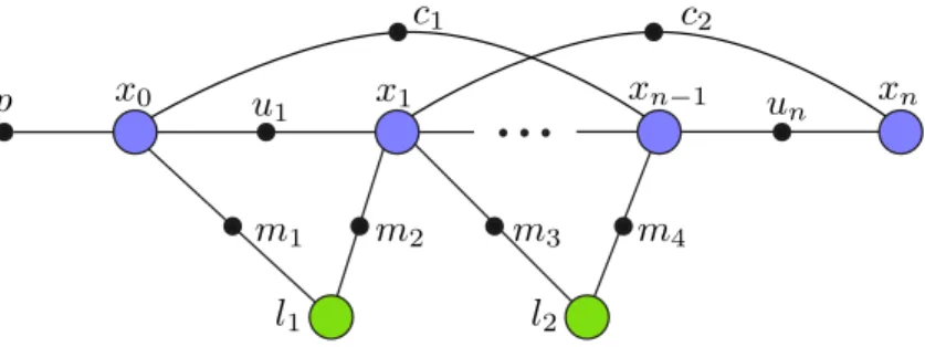
2-1 Factor graph representation of the SLAM maximum-likelihood estimation 32 2-2 Pose-graph SLAM . . . 35

3-1 Computing the Powell’s Dog-Leg update step . . . 45

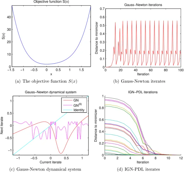
3-2 Failure of the Gauss-Newton method . . . 56

3-3 Exact trust-region and Powell’s Dog-Leg update paths . . . 61

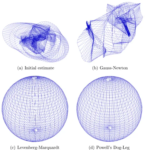
3-4 Example results for batch nonlinear least-squares methods on the sphere2500 dataset . . . 80

3-5 Incremental visual mapping using a calibrated monocular camera . . 84

4-1 An example realization of the cube dataset . . . 99

4-2 Characterizing the exactness of the relaxation Problem 9 . . . 100

5-1 Results for the cube experiments. . . 117

5-2 Visualizations of optimal solutions recovered by SE-Sync for large-scale 3D pose-graph SLAM datasets . . . 118

(12)

(13)

List of Tables

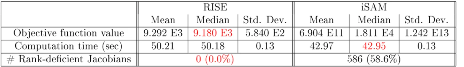
3.1 Summary of results for batch nonlinear least-squares methods on the sphere2500 dataset . . . 80 3.2 Summary of results for incremental nonlinear least-squares methods on

the sphere2500 dataset . . . 82 3.3 Summary of results for the incremental nonlinear least-squares

meth-ods in online visual mapping . . . 84 4.1 Results for large-scale pose-graph SLAM solution verification

experi-ments . . . 101 5.1 Results of applying SE-Sync to large-scale 3D pose-graph SLAM

(14)

(15)

List of Algorithms

3.1 Updating the trust-region radius ∆ . . . 59

3.2 The trust-region minimization method . . . 59

3.3 Computing the dog-leg step ℎ𝑑𝑙 . . . 63

3.4 The indefinite Gauss-Newton-Powell’s Dog-Leg algorithm . . . 65

3.5 The RISE algorithm . . . 74

3.6 The RISE2 algorithm . . . 77

5.1 The Riemannian Staircase . . . 109

5.2 Rounding procedure for solutions of Problem 11 . . . 113

(16)

(17)

Chapter 1 Introduction

1.1 Motivation

The preceding decades have witnessed remarkable advances in both the capability and reliability of autonomous robots. As a result, robotics is now on the cusp of transitioning from an academic research project to a ubiquitous technology in industry and in everyday life. Over the coming years, the increasingly widespread utilization of robotic technology in applications such as transportation [77, 130, 138], medicine [21, 126, 127], and disaster response [42, 63, 103] has tremendous potential to increase productivity, alleviate suffering, and preserve life.

At the same time however, the very applications for which robotics is poised to realize the greatest benefit typically carry a correspondingly high cost of poor performance. For example, in the case of transportation, the failure of an autonomous vehicle to function correctly may lead to destruction of property, severe injury, or even loss of life [141]. This high cost of poor performance presents a serious barrier to the widespread adoption of robotic technology in the high-impact but safety-critical applications that we would most like to address, absent some guarantee of “good behavior” on the part of the autonomous agent(s). While such guarantees (viz. of correctness, feasibility, optimality, bounded suboptimality, etc.), have long been a feature of algorithms for planning [111] and control [1, 120], to date it appears that the development of practical algorithms with guaranteed performance for robotic

(18)

perception has to a great extent remained an open problem.

One particularly salient example of this general trend is the problem of simulta-neous localization and mapping (SLAM). As its name suggests, this is the perceptual problem in which a robot attempts to estimate a model of its environment (mapping) while simultaneously estimating its position and orientation within that model (lo-calization). Mathematically, this problem entails the joint estimation of the absolute configurations of a collection of entities (typically the robot’s pose(s) and the pose(s) of any interesting object(s) discovered in the environment) in some global coordi-nate system based upon a set of noisy measurements of relative geometric relations amongst them. This latter formulation, however, immediately generalizes far beyond the estimation of maps: in this broader view, SLAM is the problem of estimating global geometry from local measurements. The need to perform such geometric esti-mation is ubiquitous throughout robotics and autoesti-mation, as the resulting estimates are required for such fundamental functions as planning, navigation, object learning and discovery, and manipulation (cf. e.g. [131] generally). In consequence, SLAM is an essential enabling technology for mobile robots, and the development of fast and reliable algorithms for solving this problem is of considerable practical import.

Current state-of-the-art approaches to SLAM formulate this inference problem as an instance of maximum-likelihood estimation (MLE) under an assumed probability distribution for the errors corrupting a robot’s available measurements [118]. This formulation is attractive from a theoretical standpoint due to the powerful analytical framework and strong performance guarantees that maximum-likelihood estimation affords [43]. However, actually obtaining the maximum-likelihood estimate requires solving a high-dimensional nonconvex nonlinear program, which is a fundamentally hard computational problem. As a result, these algorithms instead focus upon the ef-ficient computation of (hopefully) high-quality approximate solutions by applying fast first- or second-order smooth numerical optimization methods to compute a critical point of the SLAM MLE. This approach is particularly attractive because the rapid convergence speed of second-order optimization methods [96], together with their ability to exploit the measurement sparsity that typically occurs in naturalistic

(19)

prob-(a) Optimal estimate (b) Suboptimal critical point

(c) Suboptimal critical point (d) Suboptimal critical point

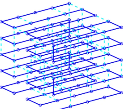
Figure 1-1: Examples of suboptimal estimates in pose-graph SLAM. This figure shows several estimates for the trajectory of a robot as it enters and explores a multi-level parking garage, obtained as critical points of the corresponding pose-graph SLAM maximum-likelihood estimation. Fig. 1-1(a) shows the globally optimal trajectory estimate, obtained using SE-Sync (Chp. 5), while 1-1(b), 1-1(c), and 1-1(d) are sub-optimal critical points of the MLE obtained using local search.

lem instances [34], enables these techniques to scale effectively to large problem sizes while maintaining real-time operation. Indeed, there now exist a variety of mature algorithms and software libraries based upon this approach that are able to process SLAM problems involving tens of thousands of latent states in a matter of minutes using only a single thread on a commodity processor [35, 52, 68, 73, 75, 84, 107].

However, while the efficient computation that these fast approximate algorithms afford has been crucial in reducing SLAM to a practically-solvable problem, this computational expedience comes at the expense of reliability, as the restriction to local search leaves these methods vulnerable to convergence to significantly suboptimal critical points. Indeed, it is not difficult to find even fairly simple real-world examples where estimates recovered by local search methods are so poor as to be effectively unusable (Fig. 1-1). Given the crucial role that the estimates supplied by SLAM

(20)

systems play in enabling the basic functions of mobile robots, this lack of reliability in existing SLAM inference methods represents a serious barrier to the development of robust autonomous agents generally.

1.2 Contributions

Motivated by the preceding considerations, this thesis addresses the problem of devel-oping algorithms for SLAM that preserve the computational speed of existing state-of-the-art techniques while additionally providing explicit guarantees on the quality of the recovered estimates. Our contributions are threefold:

1. We develop RISE, an incremental trust-region method for robust online sparse least-squares estimation, to perform fast and numerically stable local optimiza-tion in the online SLAM setting. RISE preserves the computaoptimiza-tional speed and superlinear convergence rate of existing state-of-the-art online SLAM solvers while providing superior robustness to nonlinearity and numerical ill-conditioning; in particular, RISE is globally convergent under very mild hypotheses (namely, that the objective is twice-continuously differentiable with bounded sublevel sets). We show experimentally that RISE’s enhanced convergence proper-ties lead to dramatically improved performance versus existing state-of-the-art techniques for SLAM problems exhibiting strong nonlinearities, such as those encountered in visual mapping or when employing robust cost functions [104, 105, 107].

2. We address the lack of a priori performance guarantees when applying local optimization methods to the nonconvex SLAM maximum-likelihood estima-tion by developing a post hoc verificaestima-tion method for computaestima-tionally certifying the correctness (i.e. global optimality) of a recovered estimate for pose-graph SLAM. The crux of our approach is the development of a (convex) semidefinite relaxation of the SLAM MLE that is frequently exact in the low to moderate measurement noise regime. We show that when exactness holds, it is

(21)

straight-forward to construct an optimal solution 𝑍* _{for this relaxation from an optimal}

solution 𝑥* _{of the SLAM problem; the dual solution 𝑍}* _{(whose optimality can}

be verified directly post hoc) then serves as a certificate of optimality for the solution 𝑥* _{from which it was constructed. Extensive evaluation on a variety}

of simulated and real-world pose-graph SLAM datasets shows that this verifi-cation method succeeds in certifying optimal solutions across a broad spectrum of operating conditions, including those typically encountered in application [26, 109, 136].

3. We develop SE-Sync, a pose-graph SLAM inference algorithm that employs a fast purpose-built optimization method to directly solve the aforementioned semidefinite relaxation, and thereby recover a certifiably globally optimal so-lution of the SLAM MLE whenever exactness holds. As in the case of our verification technique, extensive empirical evaluation on a variety of simulated and real-world datasets shows that SE-Sync is capable of recovering globally optimal pose-graph SLAM solutions across a broad spectrum of operating con-ditions (including those typically encountered in application), and does so at a computational cost that scales comparably with that of the fast Newton-based local search techniques that form the basis of current state-of-the-art SLAM algorithms [109].

Collectively, the algorithms developed herein provide fast and robust inference and verification methods for pose-graph SLAM in both the online and offline settings, and can be straightforwardly incorporated into existing concurrent filtering and smoothing architectures [146]. The result is a framework for real-time mapping and navigation that preserves the computational speed of current state-of-the-art techniques while delivering certifiably correct solutions.

(22)

1.3 Notation and mathematical preliminaries

Before proceeding, in this section we collect some notation and mathematical prelim-inaries that will be of use throughout the remainder of this thesis.

Miscellaneous sets: The symbol Z denotes the integers, N the nonnegative integers, Q the rational numbers, R the real numbers, and we write [𝑛] , {1, . . . , 𝑛} for 𝑛 > 0 as a convenient shorthand notation for sets of indexing integers. We use |𝑆| to denote the cardinality of a set 𝑆.

Differential geometry and Lie groups: We will encounter several smooth manifolds and Lie groups, and will often make use of both the intrinsic and extrinsic formulations of the same manifold as convenience dictates; our notation will generally be consistent with that of [144] in the former case and [55] in the latter. When consid-ering an extrinsic realization ℳ ⊆ R𝑑_{of a manifold ℳ as an embedded submanifold}

of a Euclidean space and a function 𝑓 : R𝑑_{→ R, it will occasionally be important for}

us to distinguish the notions of 𝑓 considered as a function on R𝑑 _{and 𝑓 considered as}

a function on the submanifold ℳ; in these cases, to avoid confusion we will always reserve ∇𝑓 and ∇2_𝑓 _{for the gradient and Hessian of 𝑓 with respect to the usual}

metric on R𝑑_{, and write grad 𝑓 and Hess 𝑓 to refer to the Riemannian gradient and}

Hessian of 𝑓 considered as a function on ℳ (equipped with the metric inherited from its embedding) [10].

We let O(𝑑), SO(𝑑), and SE(𝑑) denote the orthogonal, special orthogonal, and special Euclidean groups in dimension 𝑑, respectively. For computational convenience we will often identify the (abstract) Lie groups O(𝑑) and SO(𝑑) with their realizations as the matrix groups:

O(𝑑) ∼= {𝑅 ∈ R𝑑×𝑑 | 𝑅T𝑅 = 𝑅𝑅T = 𝐼𝑑} (1.1a)

(23)

and SE(𝑑) with the semidirect product R𝑑

o SO(𝑑) with group operations:

(𝑡1, 𝑅1) · (𝑡2, 𝑅2) = (𝑡1+ 𝑅1𝑡2, 𝑅1𝑅2). (1.2a)

(𝑡, 𝑅)−1 = (−𝑅−1𝑡, 𝑅−1). (1.2b)

The set of orthonormal 𝑘-frames in R𝑛 (𝑘 ≤ 𝑛):

St(𝑘, 𝑛) ,{︀𝑌 ∈ R𝑛×𝑘 | 𝑌T_{𝑌 = 𝐼} 𝑘

}︀

(1.3) is also a smooth compact manifold, called the Stiefel manifold; we equip St(𝑘, 𝑛) with the Riemannian metric induced by its embedding into R𝑛×𝑘 _{[3, Sec. 3.3.2].}

Linear algebra: In addition to the matrix groups defined above, we write Sym(𝑑) for the set of real 𝑑×𝑑 symmetric matrices; 𝐴 ⪰ 0 and 𝐴 ≻ 0 indicate that 𝐴 ∈ Sym(𝑑) is positive semidefinite and positive definite, respectively. For general matrices 𝐴 and 𝐵, 𝐴 ⊗ 𝐵 indicates the Kronecker (matrix tensor) product, 𝐴† the Moore-Penrose pseudoinverse, and vec(𝐴) the vectorization operator that concatenates the columns of 𝐴 [59, Sec. 4.2]. We write 𝑒𝑖 ∈ R𝑑 and 𝐸𝑖𝑗 ∈ R𝑚×𝑛 for the 𝑖th unit coordinate

vector and (𝑖, 𝑗)-th unit coordinate matrix, respectively, and 1𝑑 ∈ R𝑑 for the all-1’s

vector.

We will also frequently consider various (𝑑 × 𝑑)-block-structured matrices, and it will be useful to have specialized operators for them. To that end, given square matrices 𝐴𝑖 ∈ R𝑑×𝑑 for 𝑖 ∈ [𝑛], we let Diag(𝐴1, . . . , 𝐴𝑛) denote their matrix direct

sum. Conversely, given a (𝑑 × 𝑑)-block-structured matrix 𝑀 ∈ R𝑑𝑛×𝑑𝑛 _{with 𝑖𝑗-block}

𝑀𝑖𝑗 ∈ R𝑑×𝑑, we let BlockDiag𝑑(𝑀 ) denote the linear operator that extracts 𝑀’s

(𝑑 × 𝑑)-block diagonal: BlockDiag_𝑑_{(𝑀 ) , Diag(𝑀}11, . . . , 𝑀𝑛𝑛) = ⎛ ⎜ ⎜ ⎜ ⎝ 𝑀11 ... 𝑀𝑛𝑛 ⎞ ⎟ ⎟ ⎟ ⎠ (1.4)

(24)

and SymBlockDiag𝑑 its corresponding symmetrized form:

SymBlockDiag_𝑑_{(𝑀 ) ,} 1

2BlockDiag𝑑(︀𝑀 + 𝑀

T_{)︀ .} _(1.5)

Finally, we let SBD(𝑑, 𝑛) denote the set of symmetric (𝑑 × 𝑑)-block-diagonal matrices in R𝑑𝑛×𝑑𝑛_:

SBD(𝑑, 𝑛) , {Diag(𝑆1, . . . , 𝑆𝑛) | 𝑆1, . . . , 𝑆𝑛 ∈ Sym(𝑑)}. (1.6)

Graph theory: An undirected graph is a pair 𝐺 = (𝒱, ℰ), where 𝒱 is a finite set and ℰ is a set of unordered pairs {𝑖, 𝑗} with 𝑖, 𝑗 ∈ 𝒱 and 𝑖 ̸= 𝑗. Elements of 𝒱 are called vertices or nodes, and elements of ℰ are called edges. An edge 𝑒 = {𝑖, 𝑗} ∈ ℰ is said to be incident to the vertices 𝑖 and 𝑗; 𝑖 and 𝑗 are called the endpoints of 𝑒. We write 𝛿(𝑣) for the set of edges incident to a vertex 𝑣.

A directed graph is a pair ⃗𝐺 = (𝒱, ⃗ℰ), where 𝒱 is a finite set and ⃗ℰ ⊂ 𝒱 × 𝒱 is a set of ordered pairs (𝑖, 𝑗) with 𝑖 ̸= 𝑗.1 _{As before, elements of 𝒱 are called vertices or}

nodes, and elements of ⃗ℰ are called (directed) edges or arcs. Vertices 𝑖 and 𝑗 are called the tail and head of the directed edge 𝑒 = (𝑖, 𝑗), respectively; 𝑒 is said to leave 𝑖 and enter 𝑗 (we also say that 𝑒 is incident to 𝑖 and 𝑗 and that 𝑖 and 𝑗 are 𝑒’s endpoints, as in the case of undirected graphs). We let 𝑡, ℎ: ⃗ℰ → 𝒱 denote the functions mapping each edge to its tail and head, respectively, so that 𝑡(𝑒) = 𝑖 and ℎ(𝑒) = 𝑗 for all 𝑒 = (𝑖, 𝑗) ∈ ⃗ℰ. Finally, we again let 𝛿(𝑣) denote the set of directed edges incident to 𝑣, and 𝛿−_(𝑣) _{and 𝛿}+_(𝑣) _{denote the sets of edges leaving and entering vertex 𝑣,}

respectively.

Given an undirected graph 𝐺 = (𝒱, ℰ), we can construct a directed graph ⃗𝐺 = (𝒱, ⃗ℰ) from it by arbitrarily ordering the elements of each pair {𝑖, 𝑗} ∈ ℰ; the graph

⃗

𝐺 so obtained is called an orientation of 𝐺.

A weighted graph is a triplet 𝐺 = (𝒱, ℰ, 𝑤) comprised of a graph (𝒱, ℰ) and a weight function 𝑤 : ℰ → R defined on the edges of this graph; since ℰ is finite, we can

1_{Note that our definitions of directed and undirected graphs explicitly exclude the possibility of}

(25)

alternatively specify the weight function 𝑤 by simply listing its values {𝑤𝑖𝑗}𝑖𝑗∈ℰ on

each edge. Any unweighted graph can be interpreted as a weighted graph equipped with the uniform weight function 𝑤 ≡ 1.

We can associate to a directed graph ⃗𝐺 = (𝒱, ⃗ℰ) with 𝑛 = |𝒱| and 𝑚 = |⃗ℰ| the incidence matrix 𝐴( ⃗𝐺) ∈ R𝑛×𝑚 whose rows and columns are indexed by 𝑖 ∈ 𝒱 and

𝑒 ∈ ⃗ℰ, respectively, and whose elements are determined by:

𝐴( ⃗𝐺)𝑖𝑒 = ⎧ ⎪ ⎪ ⎪ ⎪ ⎪ ⎨ ⎪ ⎪ ⎪ ⎪ ⎪ ⎩ +1, 𝑒 ∈ 𝛿+_(𝑖) −1, 𝑒 ∈ 𝛿−(𝑖), 0, otherwise. (1.7)

Similarly, we can associate to an undirected graph 𝐺 an oriented incidence matrix 𝐴(𝐺) obtained as the incidence matrix of any of its orientations ⃗𝐺. We obtain a re-duced (oriented) incidence matrix

¯

𝐴(𝐺)by removing the final row from the (oriented) incidence matrix 𝐴(𝐺).

Finally, we can associate to a weighted undirected graph 𝐺 = (𝒱, ℰ, 𝑤) with 𝑛 = |𝒱| the Laplacian matrix 𝐿(𝐺) ∈ Sym(𝑛) whose rows and columns are indexed by 𝑖 ∈ 𝒱, and whose elements are determined by:

𝐿(𝐺)𝑖𝑗 = ⎧ ⎪ ⎪ ⎪ ⎪ ⎪ ⎨ ⎪ ⎪ ⎪ ⎪ ⎪ ⎩ ∑︀ 𝑒∈𝛿(𝑖)𝑤(𝑒), 𝑖 = 𝑗, −𝑤(𝑒), 𝑖 ̸= 𝑗 and 𝑒 = {𝑖, 𝑗} ∈ ℰ, 0, otherwise. (1.8)

A straightforward computation shows that the Laplacian of a weighted graph 𝐺 and the incidence matrix of one of its orientations ⃗𝐺 are related by:

𝐿(𝐺) = 𝐴( ⃗𝐺)𝑊 𝐴( ⃗𝐺)T, (1.9)

where 𝑊 , Diag(𝑤(𝑒1), . . . , 𝑤(𝑒𝑚)) is the diagonal matrix containing the weights of

(26)

Probability and statistics: We write 𝒩 (𝜇, Σ) for the multivariate Gaussian distribution with mean 𝜇 ∈ R𝑑 and covariance matrix 0 ⪯ Σ ∈ Sym(𝑑), and

Langevin(𝜅, 𝑀 ) for the isotropic Langevin distribution with mode 𝑀 ∈ SO(𝑑) and concentration parameter 𝜅 ≥ 0; the latter is the distribution on SO(𝑑) whose proba-bility density function is given by:

𝑝(𝑅; 𝜅, 𝑀 ) = 1 𝑐𝑑(𝜅)

exp(︀𝜅 tr(𝑀T𝑅))︀ (1.10)

with respect to the Haar measure [31]. With reference to a hidden parameter 𝑋 whose value we wish to infer, we will write

¯

𝑋 for its true (latent) value, ˜𝑋 to denote a noisy observation of

¯

𝑋, and ˆ𝑋 to denote an estimate of ¯ 𝑋.

1.4 Overview

The remainder of this thesis is organized as follows. Chapter 2 provides a review of the maximum-likelihood formulation of the full or smoothing SLAM problem that will form the basis of our subsequent development, its representation by means of probabilistic graphical models, and an overview of related work on the formulation and solution of this problem. Chapter 3 develops the RISE algorithm. Chapter 4 introduces the semidefinite relaxation that will form the basis of our work on pose-graph SLAM, and then shows how to exploit this relaxation to produce our solution verification method. Chapter 5 continues with the development of SE-Sync. Finally, Chapter 6 concludes with a summary of this thesis’s contributions and a discussion of future research directions.

(27)

Chapter 2 A review of graphical SLAM

This chapter provides a brief self-contained overview of the maximum-likelihood for-mulation of the full or smoothing SLAM problem that will form the foundation of our subsequent development.1 _{We begin with a first-principles derivation of this problem}

formulation in Section 2.1, and describe its corresponding representation via factor graphs in Section 2.2. Section 2.3 discusses the important special case of pose-graph SLAM and its associated specialized graphical model, the pose-graph. Finally, Section 2.4 provides an overview of prior work on the formulation and solution of the SLAM inference problem, focusing in particular on graphical SLAM techniques. Readers already familiar with this general background material may safely skip ahead to the remaining chapters of this thesis.

2.1 The maximum-likelihood formulation of SLAM

Here we review the maximum-likelihood formulation of the full or smoothing SLAM problem. Our presentation will be fairly abstract in order to emphasize the broad generality of the approach, as well as the essential mathematical features of the result-ing inference problem. Readers interested in a more concrete or application-oriented

1_{In the robotics literature, this formulation is often referred to as graphical SLAM [53], as current}

state-of-the-art algorithms and software libraries for solving it heavily exploit its representation in the form of a probabilistic graphical model [71] to achieve both efficient inference (through the exploitation of conditional independence relations as revealed in the graph’s edge structure) and concise problem specification.

(28)

introduction, or alternative formulations of the SLAM problem, are encouraged to consult the excellent standard reference [131, Chp. 10] or the survey articles [37, 118]. Let us consider a robot exploring some initially unknown environment. As the robot explores, it uses a complement of onboard sensors to collect a set of mea-surements ˜𝑍 = {˜𝑧𝑖}𝑚𝑖=1 that provide information about some set of latent states

Θ = {𝜃𝑖}𝑛𝑖=1 that we would like to estimate. Typically, the latent states Θ are

com-prised of the sequence of poses2 _{that the robot moves through as it explores the}

environment, together with a collection of parameters that describe any interesting environmental features that the robot discovers during its exploration (these may include, for example, the positions of any distinctive landmarks, or the poses of any objects, that the robot detects using e.g. an onboard laser scanner or camera system). In general, each measurement ˜𝑧𝑖 collected by one of the sensors carried aboard

a mobile robot arises from the interaction of a small subset Θ𝑖 = {𝜃𝑖𝑘}

𝑛𝑖

𝑘=1 of the

complete set Θ of latent states that we are interested in estimating. For example, the position measurement reported by a GPS receiver (if one is available) depends only upon the robot’s immediate position at the moment that measurement is obtained (and not, e.g., on its position five minutes previously). Similarly, an individual mea-surement collected by a laser scanner provides information about the location of a point relative to the scanner itself, and so depends only upon the absolute pose of that scanner and the absolute position of that point in some global coordinate frame at the moment the measurement is collected.

We can make these dependencies explicit by associating to the 𝑖th measurement ˜

𝑧𝑖 a corresponding measurement function ℎ𝑖(·) that encodes how the latent states Θ𝑖

upon which that measurement depends combine to produce an idealized exact (i.e. noiseless) observation 𝑧𝑖:

𝑧𝑖 = ℎ𝑖(Θ𝑖); (2.1)

in this equation, the functional form of ℎ𝑖(·) (including its arity), as well as the

domains in which the latent states Θ𝑖 = {𝜃𝑖1, . . . , 𝜃𝑖𝑘} and idealized measurement 𝑧𝑖

2_{The pose of an object is its position and orientation in an ambient Euclidean space R}𝑑_{; this is}

(29)

lie, depend upon what kind of measurement is being described, and are determined by the geometry of the sensing apparatus. For example, in the case of odometry measurements, ℎ𝑖(·) is binary (since an odometry measurement relates two robot

poses), Θ𝑖 = {𝑥𝑖1, 𝑥𝑖2} with 𝑥𝑖1, 𝑥𝑖2 ∈ SE(𝑑), and the measurement function ℎ𝑖(·) is given explicitly by ℎ(𝑥𝑖1, 𝑥𝑖2) = 𝑥

−1

𝑖1 𝑥𝑖2, where the operations on the right-hand side of this equation are to be interpreted using SE(𝑑)’s group inversion and multiplication operations (1.2). Similarly, in the case that (2.1) describes a measurement made with a monocular camera, ℎ𝑖(·) is a ternary measurement function ℎ𝑖(𝑡𝑖, 𝑥𝑖, 𝐾𝑖) encoding

the pinhole camera projection model [58, Sec. 6.1], which describes how the camera’s pose 𝑥𝑖 ∈ SE(3) and intrinsic calibration 𝐾𝑖 ∈ R3×3, together with the position of

the imaged point 𝑡𝑖 ∈ R3 in the world, determine the projection 𝑧𝑖 ∈ R2 of that point

onto the camera’s image plane.

Of course, in reality each of the measurements ˜𝑧𝑖 is corrupted by some amount of

measurement noise, and so in practice, following the paradigm of probabilistic robotics [131, Chp. 1], we attempt to explicitly account for the presence of this measurement error (and our resulting uncertainty about the value of the “true” measurement 𝑧𝑖) by

considering each observation ˜𝑧𝑖 to be a random realization drawn from a conditional

measurement distribution:

˜

𝑧𝑖 ∼ 𝑝𝑖(·|Θ𝑖); (2.2)

here the specific form of the distribution on the right-hand side of (2.2) is determined by both the idealized measurement model (2.1) and the form of the noise that is hypothesized to be corrupting the observation ˜𝑧𝑖. For example, under the common

assumption that ˜𝑧𝑖 is the result of corrupting an idealized measurement 𝑧𝑖 = ℎ𝑖(Θ𝑖)

with additive mean-zero Gaussian noise with covariance Σ𝑖 ∈ Sym(𝑑𝑖):

˜

𝑧𝑖 = ℎ𝑖(Θ𝑖) + 𝜖𝑖 𝜖𝑖 ∼ 𝒩 (0, Σ𝑖), (2.3)

(30)

(2.2) can be written in closed form as: 𝑝𝑖(˜𝑧𝑖|Θ𝑖) = (2𝜋)−𝑑𝑖/2|Σ𝑖|−𝑑𝑖/2exp (︂ −1 2‖˜𝑧𝑖− ℎ𝑖(Θ𝑖)‖ 2 Σ𝑖 )︂ , (2.4) where ‖𝑥‖Σ , √

𝑥T_Σ𝑥 denotes the Mahalanobis distance determined by Σ. Explicit

forms of the conditional densities (2.2) corresponding to other choices of noise model can be derived in an analogous fashion.

Now, under the assumption that the errors corrupting each individual measure-ment ˜𝑧𝑖 are independent, the conditional distribution 𝑝( ˜𝑍|Θ) for the complete set of

observations ˜𝑍 given the complete set of latent states Θ factors as the product of the individual measurement distributions (2.2):

𝑝( ˜𝑍|Θ) =

𝑚

∏︁

𝑖=1

𝑝𝑖(˜𝑧𝑖|Θ𝑖). (2.5)

By virtue of (2.5), we may therefore obtain a maximum-likelihood estimate ˆΘMLE for

the latent states Θ based upon the measurements ˜𝑍 according to: Problem 1 (SLAM maximum-likelihood estimation).

ˆ Θ_MLE _{, argmax} Θ 𝑝( ˜𝑍|Θ) = argmin Θ 𝑚 ∑︁ 𝑖=1 − ln 𝑝𝑖(˜𝑧𝑖|Θ𝑖). (2.6)

Our focus in the remainder of this thesis will be on the development of efficient and reliable methods for actually carrying out the minimization indicated in (2.6).

2.2 The factor graph model of SLAM

Equation (2.5) provides a decomposition of the joint conditional density 𝑝( ˜𝑍|Θ)that appears in the SLAM maximum-likelihood estimation Problem 1 in terms of the conditional densities (2.2) that model the generative process for each individual mea-surement ˜𝑧𝑖. In general, the existence of a factorization of a joint probability

(31)

variables that distribution describes. It is often convenient to associate to such a factorization a probabilistic graphical model [71], a graph whose edge structure makes explicit the corresponding conditional independence relations implied by that fac-torization. Conversely, one can also use a probabilistic graphical model to specify a complicated joint distribution by describing how it can be “wired together” from simpler conditional distributions, as in (2.5). Here we briefly describe one class of probabilistic graphical models, factor graphs [74, 82], and their use in modeling the SLAM problem (2.6), following the presentation given in our prior work [106, 110]. Readers interested in a more detailed exposition of the use of factor graph models in SLAM are encouraged to consult the excellent references [33, 34].

Formally, a factor graph is a bipartite graph that encodes the factorization of a function 𝑓(Θ) of several variables Θ = {𝜃1, . . . , 𝜃𝑛}: given the factorization

𝑓 (Θ) =

𝑚

∏︁

𝑖=1

𝑓𝑖(Θ𝑖), (2.7)

with Θ𝑖 ⊆ Θfor all 1 ≤ 𝑖 ≤ 𝑚, the corresponding factor graph 𝒢 = (ℱ, Θ, ℰ) is:

ℱ = {𝑓1, . . . , 𝑓𝑚},

Θ = {𝜃1, . . . , 𝜃𝑛},

ℰ = {{𝑓𝑖, 𝜃𝑗} | 𝑖 ∈ [𝑚], 𝜃𝑗 ∈ Θ𝑖} .

(2.8)

By (2.8), the elements of the vertex set ℱ (called factor nodes) are in one-to-one correspondence with the factors 𝑓𝑖(·)in (2.7), the elements of the vertex set Θ (called

variable nodes) are in one-to-one correspondence with the arguments 𝜃𝑗 of 𝑓(·), and

𝒢 has an edge between a factor node 𝑓𝑖 and a variable node 𝜃𝑗 if and only if 𝜃𝑗 is an

argument of 𝑓𝑖(·) in (2.7).

Fig. 2-1 depicts a representative snippet from the factor graph model of a typical pose-and-landmark SLAM problem. The use of such models provides several advan-tages as a means of specifying the SLAM inference problem (2.6). First, the edge set in a factor graph explicitly encodes the conditional independence relations amongst

(32)

Figure 2-1: The factor graph representation of the SLAM maximum-likelihood esti-mation Problem 1. This figure depicts a representative snippet from the factor graph model of a typical pose-and-landmark SLAM problem. Here variable nodes are shown as large circles and factor nodes as small solid circles. The variables consist of robot poses 𝑥 and landmark positions 𝑙, and the factors are odometry measurements 𝑢, a prior 𝑝 on the initial robot pose 𝑥0, loop closure measurements 𝑐, and landmark

measurements 𝑚. Each of the factor nodes in this diagram corresponds to a factor 𝑝𝑖(˜𝑧𝑖|Θ𝑖)on the right-hand sides of (2.5) and (2.6).

the random variables that it models. The deft exploitation of these conditional in-dependences is crucial for the design of efficient algorithms for performing inference over the probabilistic generative model that the factor graph encodes. By making them explicit, factor graphs thus expose these independence relations in a way that can be algorithmically exploited to enable the automatic generation of efficient in-ference procedures [67]. Second, because factor graphs are abstracted at the level of probability distributions, they provide a convenient modular architecture that en-ables the straightforward integration of heterogeneous data sources, including both sensor observations and prior knowledge (specified in the form of prior probability distributions). This “plug-and-play” framework provides a formal model that greatly simplifies the design and implementation of complex systems while ensuring the cor-rectness of the associated inference procedures. Finally, factor graphs lend themselves to straightforward implementation and manipulation in software via objected-oriented programming, making them a convenient formalism to apply in practice.

In light of these advantages, it has become common practice to specify SLAM inference problems of the form (2.6) in terms of their factor graph representations (or specializations thereof), and indeed current state-of-the-art inference algorithms and software libraries typically require a specification of this form [52, 68, 75, 107].

(33)

Consequently, in the sequel we will assume the availability of such representations without comment, and will exploit several of their graph-theoretic properties in the design of our algorithms.

2.3 Pose-graph SLAM

One particularly important special case of the general maximum-likelihood SLAM formulation (2.6) is pose-graph SLAM [53]; in this case, the latent states of interest are a collection of robot poses 𝑥1, . . . , 𝑥𝑛 ∈ SE(𝑑), and the observations consist of

noisy measurements ˜𝑥𝑖𝑗 ∈ SE(𝑑) of a subset of the pairwise relative transforms 𝑥−1𝑖 𝑥𝑗

between them. Letting ⃗ℰ ⊂ [𝑛]×[𝑛] denote the subset of ordered pairs3_{for which there}

is an available measurement ˜𝑥𝑖𝑗, the corresponding instance of the SLAM

maximum-likelihood estimation Problem 1 is thus:

Problem 2 (Pose-graph SLAM maximum-likelihood estimation). ˆ 𝑥_MLE= argmin 𝑥∈SE(𝑑)𝑛 ∑︁ (𝑖,𝑗)∈ ⃗ℰ − ln 𝑝𝑖𝑗(˜𝑥𝑖𝑗|𝑥𝑖, 𝑥𝑗) (2.9)

This formulation of the SLAM problem arises when one uses measurements of the external environment as a means of estimating the relative transforms between pairs of poses at which scans were collected (as is the case, for example, when applying laser scan matching or stereoframe matching). The appeal of this formulation is that it eliminates the external environmental features from the estimation problem; as there are often orders of magnitude more environmental features than poses in a typical pose-and-landmark SLAM problem, this represents a significant savings in terms of both computation and memory. At the same time, however, it is easy to see from the structure of the pose-and-landmark factor graph in Fig. 2-1 that the estimates of the landmark locations in the environment are conditionally independent given an estimate for the set of robot poses 𝑥1, . . . 𝑥𝑛 (this follows from the fact that

3_{The ordering here is important because the measurement distributions 𝑝}_𝑖_(˜_𝑥_𝑖𝑗_|𝑥_𝑖_{, 𝑥}_𝑗₎_appearing

(34)

landmarks only connect to robot poses, and not, for example, to each other). This implies that, having obtained an estimate for the set of robot poses by solving Problem 2, reconstructing a model of the environment given this estimate reduces to solving a collection of (small) independent estimation problems, one for each environmental feature. Consequently, pose-graph SLAM provides a particularly convenient, compact and computationally efficient formulation of the SLAM problem, and for this reason has become arguably the most important and common formulation in the robotics literature.4

Now as Problem 2 specializes Problem 1, there is an associated specialization of the SLAM factor graph model of Section 2.2 to Problem 2, called a pose graph. Observe that since each factor 𝑝𝑖𝑗(˜𝑥𝑖𝑗|𝑥𝑖, 𝑥𝑗)in (2.9) has two arguments,5 every factor

node 𝑝𝑖𝑗 in the factor graph model of Problem 2 is binary. But in that case, rather

than associating pairs of variable nodes 𝑥𝑖 and 𝑥𝑗 with an explicit binary factor node

𝑝𝑖𝑗, it would serve just as well to associate 𝑥𝑖 and 𝑥𝑗 with a directed edge (𝑖, 𝑗) that

models the presence of 𝑝𝑖𝑗. Concretely then, the pose-graph model associated with

Problem 2 is the directed graph ⃗𝒢 = (𝒳 , ⃗ℰ) whose vertices 𝒳 = {𝑥𝑖}𝑛𝑖=1are in

one-to-one correspondence with the poses 𝑥𝑖 to be estimated, and whose directed edges are

in one-to-one correspondence with the binary conditional measurement distributions 𝑝𝑖𝑗(˜𝑥𝑖𝑗|𝑥𝑖, 𝑥𝑗) in (2.9). Fig. 2-2 depicts a snippet from a representative pose-graph.

Finally, the specific version of the pose-graph SLAM maximum-likelihood esti-mation Problem 2 that appears in the robotics literature typically assumes that the conditional measurement densities 𝑝𝑖𝑗(˜𝑥𝑖𝑗|𝑥𝑖, 𝑥𝑗) correspond to additive mean-zero

Gaussian noise corrupting the translational observations and multiplicative noise cor-rupting the rotational observations that is obtained by exponentiating an element of

4_{Historically, pose-graph SLAM was also the first instantiation of the general maximum-likelihood}

smoothing formulation (2.6) to appear in the robotics literature, as it was this specific form of Problem 1 that appeared in the original paper proposing this paradigm [85].

(35)

𝑥1 𝑥2 𝑥3 𝑥4 𝑥5 𝑥6 𝑥𝑖 ˜ 𝑥12 𝑥˜23 ˜𝑥34 ˜ 𝑥45 ˜ 𝑥56 ˜𝑥52 ˜𝑥61

Figure 2-2: This figure depicts a representative snippet from the pose graph corre-sponding to a typical instance of pose-graph SLAM. Here the vertices and directed edges are in one-to-one correspondence with the robot poses 𝑥𝑖 and conditional

mea-surement distributions 𝑝𝑖𝑗(˜𝑥𝑖𝑗|𝑥𝑖, 𝑥𝑗) in Problem 2, respectively.

so(𝑑)sampled from a mean-zero Gaussian distribution: ˜ 𝑡𝑖𝑗 = ¯𝑡𝑖𝑗 + 𝛿 𝑡 𝑖𝑗, 𝛿 𝑡 𝑖𝑗 ∼ 𝒩 (0, Σ 𝑡 𝑖𝑗), ˜ 𝑅𝑖𝑗 = ¯ 𝑅𝑖𝑗exp(𝛿𝑖𝑗𝑅), 𝛿 𝑅 𝑖𝑗 ∼ 𝒩 (0, Σ 𝑅 𝑖𝑗), (2.10) where ¯ 𝑥𝑖𝑗 = (

¯𝑡𝑖𝑗,𝑅¯𝑖𝑗) ∈ SE(𝑑) denotes the true (latent) value of the 𝑖𝑗-th relative transform. The appeal of the measurement model (2.10) is that the assumption of Gaussian sensor noise leads to a maximum-likelihood estimation (2.9) that takes the form of a sparse nonlinear least-squares problem:

ˆ 𝑥 = argmin 𝑥∈SE(𝑑)𝑛 ∑︁ (𝑖,𝑗)∈ ⃗ℰ ⃦ ⃦ ⃦log (︁ 𝑅−1_𝑗 𝑅𝑖𝑅˜𝑖𝑗 )︁⃦ ⃦ ⃦ 2 Σ𝑅 𝑖𝑗 +⃦⃦˜𝑡_𝑖𝑗 − 𝑅−1_𝑖 (𝑡_𝑗 − 𝑡_𝑖) ⃦ ⃦ 2 Σ𝑡 𝑖𝑗 . (2.11)

Sparse nonlinear least-squares problems of this form can be processed very efficiently in practice using sparsity-exploiting second-order optimization methods [96].

2.4 Overview of related work

As befits one of the most important problems in robotics, there is a vast body of prior work on SLAM. Since our interest in this thesis is in the development of methods for the exact solution of the maximum-likelihood formulation of this problem (2.6), our coverage here will focus primarily on work related to the development of this specific

(36)

formalism and algorithms for its exact solution. Readers interested in a broader overview of prior work on SLAM, including a more detailed description of alternative (although now largely outdated) formulations, or a discussion of other aspects of the problem unrelated to the solution of (2.6), are encouraged to consult the standard references [131, Chp. 10] and [37] and the excellent recent surveys [22, 118].

Geodesy and photogrammetry

Given that one of the principal motivations for the development of SLAM was to equip robots with the means of generating maps, it is perhaps unsurprising that estimation problems similar to (2.6) first arose in the context of geodesy. Indeed the specific formulation of Problem 1 (viz., the estimation of the geometric configuration of a set of states by means of maximum-likelihood estimation over a network of measurements of relative geometric relations, cf. Fig. 2-1) dates at least as far back as 1818, when Gauss applied this estimation procedure (in the form of least-squares estimation under the assumption of additive Gaussian errors) as part of his celebrated triangulation of the Kingdom of Hanover [56, pg. 56].6 _{This basic idea of mapping}

by applying maximum-likelihood estimation to relative geometric measurements in (often continent-scale) triangulation networks subsequently formed the foundation of geodetic mapping methods from the mid-19th century until the widespead adoption of GPS.7 _{Over a century later, in the late 1950s essentially the same estimation}

procedure was applied to photogrammetry (in form of the photogrammetric bundle method, i.e. bundle adjustment [135]) for application to aerial cartography [17, 18]. However, despite the historical precedence of these geodetic and photogrammetric methods, the robotics community appears to have developed early formulations of SLAM largely independently of them.

6_{In fact, it was actually Gauss’s interest in the solution of this first SLAM problem (as we would}

understand it today) that catalyzed some of his later work in the development of the method of least squares [47].

7_{Interested readers are encouraged to consult the recent survey [4] for a very interesting discussion}

(37)

EKF-SLAM

Within the field of robotics itself, the earliest formulation of the spatial perception problem as a probabilistic inference problem over a network of uncertain geometric relations amongst several entities is due to the series of seminal papers [29, 115, 116]; these proposed to explicitly represent the uncertainty in the estimated spatial rela-tions (including the correlarela-tions amongst them) by maintaining a jointly Gaussian belief over them, and updating this belief using an extended Kalman filter (EKF) [69]. Consequently, the earliest operational SLAM systems were based on this EKF-SLAM formalism [78, 94]. However, it quickly became apparent that EKF-SLAM suffers from two serious drawbacks. First, the standard formulation of the Kalman Filter used in EKF-SLAM marginalizes all but the current robot pose from the estimated states; as can be seen by applying the elimination algorithm [71, Chp. 9] to the odo-metric backbone in the factor graph model shown in Fig. 2-1, this marginalization leads to a completely dense state covariance matrix. Since general (i.e. dense) Kalman filter measurement updates have 𝑂(𝑛2₎computational cost, vanilla EKF-SLAM

tech-niques do not scale well to maps containing more than a few hundred states. The second serious drawback concerns the incorporation of observations corresponding to nonlinear measurement functions (2.1): in the extended Kalman filter, nonlinear mea-surements are fused using a linearization of the measurement function ℎ𝑖(·)evaluated

at the current state estimate, and then discarded. In the context of EKF-SLAM, robot pose estimates can be subject to significant drift after dead-reckoning during exploratory phases; when these high-error pose estimates are used to linearize ℎ𝑖(·)

in order to fuse new measurements and then subsequently marginalized, these erro-neous linearizations then become irreversibly baked into all subsequent joint state estimates. While the former of these two drawbacks can be mitigated to some extent through the use of a (possibly approximate) sparse information form of the extended Kalman filter [41, 129, 142], the latter is intrinsic to the filtering paradigm, and is well-known to lead to inconsistency in the resulting SLAM estimates [6, 60, 64].

(38)

Particle filtering methods

As an alternative to EKF-SLAM, another major SLAM paradigm proposes to replace the extended Kalman filter in EKF-SLAM with a (nonparametric) sequential Monte Carlo (SMC) estimator (i.e. particle filter) [81]. This approach exploits the condi-tional independence of the environmental observations given the complete sequence of robot poses (cf. Fig. 2-1) to factor the SLAM posterior distribution into a (large) posterior distribution over the robot’s path and the product of many small posterior distributions for the individual environmental features given this path; this factor-ization enables the implementation of an efficient Rao-Blackwellized particle filter in which the estimation over the robot path is performed via sequential Monte Carlo inference, and each sample maintains a collection of independent posterior distri-butions corresponding to the environmental features via a collection of independent extended Kalman filters [91, 95]. The principal advantage of this approach versus EKF-SLAM is that it provides a formally exact method for decoupling the estima-tion of the environmental features into independent subproblems with constant time updates, and thereby avoids the quadratic computational cost associated with main-taining a single joint environmental state estimate in an EKF. Consequently, early particle-filtering-based methods for SLAM were able to scale to environments that were orders of magnitude larger than what contemporary EKF-SLAM algorithms could process [91]. However, this new approach does not come without its own set of drawbacks: unlike EKF-SLAM, in which only the current robot pose remains in the filter’s state estimate, particle-filtering SLAM methods must maintain the entire robot path in order to take advantage of the SLAM problem’s conditional indepen-dence structure. Consequently, the dimension of the robot state that must be esti-mated using SMC grows continuously as the robot operates. Since the number of samples that are required to cover a state space with a specified density grows expo-nentially in the dimension of that space, the use of sample-based SMC methods to estimate the (very high-dimensional) robot path renders these techniques vulnerable to particle depletion. Furthermore, because the sample propagation and resampling

(39)

steps in the particle filter construct the next sample set by modifying the current one, once significant estimation errors have accumulated in the sampled set of robot paths (due to e.g. the aforementioned particle depletion problem or the accumulation of significant dead-reckoning error during exploratory phases), these errors also become irreversibly baked into the filter in a manner analogous to the case of EKF-SLAM. As before, while this drawback can be alleviated to some extent through the use of more efficient proposal distributions and resampling strategies [49, 92, 117, 139], or by enabling particles to “share” maps efficiently (thereby increasing the number of samples that can be tractably maintained in the filter) [39, 40], it too is an intrin-sic limitation of performing sequential Monte Carlo over high-dimensional parameter spaces.

Graphical SLAM

In consequence of the potential inconsistency of EKF- and SMC-based methods, the SLAM community has now largely settled upon Problem 1 as the standard formula-tion of the SLAM problem: this approach elegantly addresses the major drawbacks of the previous paradigms by performing joint maximum-likelihood estimation over the entire network of states and measurements, thereby ensuring the consistency of the recovered estimates. However, actually obtaining these estimates requires solving the large-scale nonconvex nonlinear program (2.6), which is a computationally hard problem. As a result, much of the work on graphical SLAM over the preceding two decades has been devoted to the development of optimization procedures that are capable of processing large-scale instances of Problem 1 efficiently in practice.

Within robotics, the original formulation of SLAM as an instance of Problem 1 is due to Lu & Milios [85], who proposed to solve it using the Gauss-Newton method. This approach remains perhaps the most popular, with many well-known SLAM algorithms [45, 54, 68, 72, 73, 75, 84, 128] differing only in how they solve the corresponding normal equations. Lu & Milios themselves [85] originally proposed to use dense matrix inversion, but the 𝑂(𝑛3₎ computational cost of this technique is

(40)

com-putational speeds by exploiting symmetric positive definiteness and sparsity in the Gauss-Newton Hessian approximation using iterative methods such as sparse pre-conditioned conjugate gradient [35, 72] or (multiresolution) Gauss-Seidel relaxation [45]. Thrun & Montemerlo [128] exploited the sparse block structure of the Hessian in a direct method by using the Schur complement to solve first the (dense but low-dimensional) system corresponding to the robot pose update and then the (large but sparse) system corresponding to the landmark update. Grisetti et al. [54] exploited sparsity by implementing a hierarchical version of Gauss-Newton on a multiresolution pyramid and using lazy evaluation when propagating updates downward.

To further exploit sparsity, Dellaert & Kaess [34] conducted a thorough investiga-tion of direct linear-algebraic techniques for efficiently solving the sparse linear system determining the Gauss-Newton update step. One surprising result of this analysis was the primacy of variable ordering strategies as a factor in the computational cost of solving these systems; indeed, the use of fast sparse matrix factorization algorithms (such as sparse multifrontal QR [89] or Cholesky [30] decompositions) coupled with good variable ordering heuristics [32] enables these linear systems to be solved in a fraction of the time needed to simply construct it (i.e. evaluate the Jacobian or Hes-sian). These insights in turn eventually led to the development of iSAM and iSAM2 [66–68]; these methods achieve fast computation in the online version of Problem 1 by applying incremental direct updates to the linear system used to compute the Gauss-Newton update step whenever a new observation ˜𝑧𝑖 is incorporated, rather than

recomputing this linear system de novo. This completely incremental approach is the current state of the art for superlinear optimization methods for the online SLAM estimation (2.6), and is capable of solving problems involving tens of thousands of latent states in real-time on a single processor.

Alternatively, some SLAM approaches propose to solve Problem 1 using first-order methods. By omitting (approximate) Hessian operations entirely, these methods are able to scale to SLAM problems involving hundreds of thousands of latent states, although the lack of access to curvature information limits them to a much slower (linear) convergence rate. Olson et al. [98] proposed to overcome this slow

(41)

conver-gence by using a deterministic variation of Jacobi-preconditioned stochastic gradient descent in combination with a clever relative state parameterization that enables the algorithm to make more rapid progress through the state space. While originally con-ceived as a batch algorithm, Olson’s method was later adapted to the online setting through the use of spatially-varying learning rates and lazy evaluation [99]. Grisetti et al. [50] improved upon Olson’s original parameterization by ordering variables using a spanning tree through the network of constraints rather than temporally. These approaches were later unified to produce TORO [51], a state-of-the-art linear opti-mization algorithm for large-scale SLAM problems.

The state of the art

The graph-based maximum-likelihood SLAM algorithms described in the preceding subsection represent the current state of the art, providing fast and scalable infer-ence procedures for recovering high-accuracy SLAM estimates. The development and refinement of these methods has been critical in reducing SLAM to a practically-solvable problem. At the same time, however, these methods are not without their own limitations. In our view, the most serious of these concern the issue of reliability. In the online SLAM setting, incremental Gauss-Newton-based algorithms [66, 68, 100] have become the method of choice for most problems, due to their fast (super-linear) convergence rate and their ability to exploit the sequential structure of the underlying inference problem. However, it is well-known that the Gauss-Newton op-timization method upon which these algorithms are based can exhibit poor (even globally divergent [44, pg. 113]) behavior when applied to optimization problems ex-hibiting significant nonlinearity. This is frequently the case for SLAM, due to e.g. the presence of (non-Euclidean) orientation estimates in robot poses, the use of (nonlin-ear) camera projection models (2.1), and the introduction of robust loss functions [62] to attenuate the ill effects of grossly corrupted measurements, among other sources. This lack of robustness to nonlinearity presents a serious challenge to the reliable operation of these methods.

(42)

ap-plication of fast local optimization methods, which can only guarantee convergence to a first-order critical point, rather than a globally optimal solution (i.e., the actual maximum-likelihood estimate). This restriction to local rather than global solutions is particularly pernicious in the case of the SLAM maximum-likelihood estimation (2.6), where the combination of a high-dimensional state space and highly nonlinear objective give rise to complex cost surfaces containing many significantly suboptimal local minima in which these local search methods can become entrapped (Fig. 1-1). Some recent research has attempted to address this shortcoming by proposing, e.g., the use of stochastic gradient methods in conjunction with a clever state parameteri-zation [50, 51, 98, 99] in an effort to promote escape from local minima, or the use of more advanced initialization schemes [25, 27] to initiate the search (hopefully) close to the correct solution. Ultimately, however, these methods are all heuristic: at present, existing graphical SLAM algorithms provide no guarantees on the correctness of the estimates that they recover.

The remainder of this thesis is devoted to the development of algorithms for graphical SLAM that can address these limitations, while preserving the desirable computational properties of existing state-of-the-art techniques.

(43)

Chapter 3 Robust incremental least-squares

estimation

Many point estimation problems in robotics, computer vision, and machine learn-ing can be formulated as instances of the general problem of minimizlearn-ing a sparse nonlinear sum-of-squares objective. For example, the standard formulations of SLAM [131, Chp. 9] and bundle adjustment [58, 135] (corresponding to Problem 1 of Section 2.1 under the assumption of additive mean-zero Gaussian errors, as in (2.3) and (2.4)) and sparse (kernel) regularized least-squares classification and regression [9, 112] all belong to this class. For inference problems of this type, each input datum gives rise to a summand in the objective function, and therefore performing online inference (in which the data are collected sequentially and the estimate updated after the incorpo-ration of each new datum) corresponds to solving a sequence of sparse least-squares problems in which additional summands are added to the objective function over time.

In practice, these online inference problems are often solved by computing each estimate in the sequence as the solution of an independent minimization problem us-ing standard sparse least-squares techniques (most commonly Levenberg-Marquardt [80, 87, 96]). While this approach is general and produces good results, it is

(44)

tationally expensive, and does not exploit the sequential structure of the underlying inference problem; this limits its utility in real-time online applications, where speed is crucial.

More sophisticated solutions achieve faster computation by directly exploiting the sequentiality of the online inference problem. The canonical example is online gra-dient descent, which is attractive for its robustness, simplicity, and low memory and per-iteration computational costs, but its first-order rate can lead to painfully slow convergence [96]. Alternatively, some more recent work has led to the development of incrementalized Gauss-Newton methods [66, 68, 100] such as iSAM, that are specifi-cally designed to efficiently solve online least-squares estimation problems by applying direct updates to the system of equations defining the Gauss-Newton step whenever new data is acquired. This incremental approach, together with the Gauss-Newton method’s superlinear convergence rate, enables these techniques to achieve computa-tional speeds unmatched by iterated batch techniques. However, the Gauss-Newton method can exhibit poor (even globally divergent) behavior when applied to objective functions with significant nonlinearity (such as those encountered in visual mapping or when employing robust cost functions), which restricts the class of problems to which these Gauss-Newton-based methods can be reliably applied.

To that end, in this chapter we develop Robust Incremental least-Squares Esti-mation (RISE), an incrementalized version of the Powell’s Dog-Leg numerical opti-mization algorithm [96, 101] suitable for use in online sequential sparse least-squares problems. As a trust-region method (Fig. 3-1), Powell’s Dog-Leg is naturally ro-bust to objective function nonlinearity and numerical ill-conditioning, and enjoys excellent global convergence properties [28, 102, 113]; furthermore, it is known to perform significantly faster than Levenberg-Marquardt in batch sparse least-squares minimization while obtaining solutions of comparable quality [83]. By exploiting iSAM’s pre-existing functionality to incrementalize the computation of the dog-leg step, RISE maintains the speed of current state-of-the-art online sparse least-squares solvers while providing superior robustness to objective function nonlinearity and numerical ill-conditioning.

(45)

Figure 3-1: The Powell’s Dog-Leg update step ℎ𝑑𝑙 is obtained by interpolating the

(possibly approximate) Newton step ℎ𝑁 and the gradient descent step ℎ𝑔𝑑 using a

trust-region of radius ∆ centered on the current iterate 𝑥. By adapting ∆ online in response to the observed performance of the Newton steps near 𝑥, the algorithm is able to combine the rapid end-stage convergence speed of Newton-type methods with the reliability of gradient descent.

3.1 Problem formulation

We are interested in the general problem of obtaining a point estimate 𝑥*

∈ R𝑛_{of some}

quantity of interest 𝑋 as the solution of a sparse nonlinear least-squares problem: min 𝑥∈R𝑛𝑆(𝑥) 𝑆(𝑥) = 𝑚 ∑︁ 𝑖=1 𝑟𝑖(𝑥)2 = ‖𝑟(𝑥)‖2 (3.1) for 𝑟 : R𝑛

→ R𝑚 _{with 𝑚 ≥ 𝑛. Problems of this form frequently arise in probabilistic}

inference in the context of maximum likelihood (ML) or maximum a posteriori (MAP) parameter estimation; indeed, performing ML or MAP estimation over any probabil-ity distribution 𝑝: R𝑛 _{→ R}+ _{whose factor graph representation 𝒢 = (ℱ, 𝒳 , ℰ) [74] is}

sparse and whose factors are positive and bounded is equivalent to solving a sparse least-squares problem of the form (3.1) in which each summand 𝑟𝑖 corresponds to a

factor 𝑝𝑖 of 𝑝 [105]. Given the ubiquity of these models, robust and computationally

efficient methods for solving (3.1) are of significant practical import.

In the case of online inference, the input data are collected sequentially, and we wish to obtain a revised estimate for 𝑋 after the incorporation of each datum. Since

Certifiably correct SLAM

Certifiably Correct SLAM

by

David M. Rosen

B.S., California Institute of Technology (2008)

M.A., The University of Texas at Austin (2010)

Submitted to the Department of Electrical Engineering and Computer

Science

in partial fulfillment of the requirements for the degree of

Doctor of Science

at the

MASSACHUSETTS INSTITUTE OF TECHNOLOGY

September 2016

c

○

David M. Rosen, MMXVI. All rights reserved.

The author hereby grants to MIT permission to reproduce and to

distribute publicly paper and electronic copies of this thesis document

in whole or in part in any medium now known or hereafter created.

Author . . . .

Department of Electrical Engineering and Computer Science

August 31, 2016

Certified by. . . .

Professor John J. Leonard

Samuel C. Collins Professor of Mechanical and Ocean Engineering

Thesis Supervisor

Accepted by . . . .

Professor Leslie A. Kolodziejski

Chair, EECS Committee on Graduate Students

Certifiably Correct SLAM

by

David M. Rosen

Abstract

Acknowledgments

Contents

List of Figures

List of Tables

List of Algorithms

Chapter 1

Introduction

1.1 Motivation

1.2 Contributions

1.3 Notation and mathematical preliminaries

1.4 Overview

Chapter 2

A review of graphical SLAM

2.1 The maximum-likelihood formulation of SLAM

2.2 The factor graph model of SLAM

2.3 Pose-graph SLAM

2.4 Overview of related work

Chapter 3

Robust incremental least-squares

estimation

3.1 Problem formulation