Can we reconcile differences in estimates of carbon fluxes from land-use change and forestry for the 1990s?

(1)

HAL Id: hal-00303989

https://hal.archives-ouvertes.fr/hal-00303989

Submitted on 25 Feb 2008

HAL is a multi-disciplinary open access

archive for the deposit and dissemination of sci-entific research documents, whether they are pub-lished or not. The documents may come from teaching and research institutions in France or abroad, or from public or private research centers.

L’archive ouverte pluridisciplinaire HAL, est destinée au dépôt et à la diffusion de documents scientifiques de niveau recherche, publiés ou non, émanant des établissements d’enseignement et de recherche français ou étrangers, des laboratoires publics ou privés.

Can we reconcile differences in estimates of carbon

fluxes from land-use change and forestry for the 1990s?

A. Ito, J. E. Penner, M. J. Prather, C. P. de Campos, R. A. Houghton, T.

Kato, A. K. Jain, X. Yang, G. C. Hurtt, S. Frolking, et al.

To cite this version:

A. Ito, J. E. Penner, M. J. Prather, C. P. de Campos, R. A. Houghton, et al.. Can we reconcile differences in estimates of carbon fluxes from land-use change and forestry for the 1990s?. Atmospheric Chemistry and Physics Discussions, European Geosciences Union, 2008, 8 (1), pp.3843-3893. �hal-00303989�

(2)

ACPD

8, 3843–3893, 2008

Carbon fluxes from land-use change and

forestry A. Ito et al. Title Page Abstract Introduction Conclusions References Tables Figures ◭ ◮ ◭ ◮ Back Close

Full Screen / Esc

Printer-friendly Version

Interactive Discussion

EGU

Atmos. Chem. Phys. Discuss., 8, 3843–3893, 2008 www.atmos-chem-phys-discuss.net/8/3843/2008/ © Author(s) 2008. This work is licensed

under a Creative Commons License.

Atmospheric Chemistry and Physics Discussions

Can we reconcile differences in estimates

of carbon fluxes from land-use change

and forestry for the 1990s?

A. Ito1, J. E. Penner2, M. J. Prather3, C. P. de Campos4, R. A. Houghton5, T. Kato1, A. K. Jain6, X. Yang6, G. C. Hurtt7, S. Frolking7, M. G. Fearon7, L. P. Chini7, A. Wang8, and D. T. Price9

1

Frontier Research Center for Global Change, JAMSTEC, Yokohama, Japan

2

Department of Atmospheric, Oceanic and Space Sciences, University of Michigan, Ann Arbor, Michigan, USA

3

Earth System Science Department, University of California at Irvine, Irvine, California, USA

4

Petrobras Research and Development Center, Rio de Janeiro, Brazil

5

The Woods Hole Research Center, Woods Hole, Massachusetts, USA

6

Department of Atmospheric Science, University of Illinois, Urbana, Illinois, USA

7

Institute for the Study of Earth, Oceans, and Space, University of New Hampshire, Durham, New Hampshire, USA

8

Department of Renewable Resources, University of Alberta, Edmonton, Alberta, Canada

9

Natural Resources Canada, Northern Forestry Centre, Edmonton, Alberta, Canada

Received: 13 November 2007 – Accepted: 25 January 2008 – Published: 25 February 2008 Correspondence to: A. Ito (akinorii@jamstec.go.jp)

(3)

ACPD

8, 3843–3893, 2008

Full Screen / Esc

EGU

Abstract

The effect of Land Use Change and Forestry (LUCF) on terrestrial carbon fluxes can be regarded as a carbon credit or debit under the UNFCCC, but scientific uncertainty in the estimates for LUCF remains large. Here, we assess the LUCF estimates by exam-ining a variety of models of different types with different land cover change maps in the

5

1990s. Annual carbon pools and their changes are separated into different components for separate geographical regions, while annual land cover change areas and carbon fluxes are disaggregated into different LUCF activities and the biospheric response due to CO2fertilization and climate change. We developed a consolidated estimate of

the terrestrial carbon fluxes that combines book-keeping models with process-based

10

biogeochemical models and inventory estimates and yields an estimate of the global terrestrial carbon flux that is within the uncertainty range developed in the IPCC 4th As-sessment Report. We examined the USA and Brazil as case studies in order to assess the cause of differences from the UNFCCC reported carbon fluxes. Major differences in the litter and soil organic matter components are found for the USA. Differences in

15

Brazil result from assumptions about the LUC for agricultural purposes. The effects of CO₂fertilization and climate change also vary significantly in Brazil. Our consolidated estimate shows that the small sink in Latin America is within the uncertainty range from inverse models, but that the sink in the USA is significantly smaller than the in-verse models estimates. Because there are different sources of errors at the country

20

level, there is no easy reconciliation of different estimates of carbon fluxes at the global level. Clearly, further work is required to develop data sets for historical land cover change areas and models of biogeochemical changes for an accurate representation of carbon uptake or emissions due to LUC.

(4)

ACPD

8, 3843–3893, 2008

Full Screen / Esc

EGU

1 Introduction

Changes in the carbon pools for the terrestrial biosphere result in the uptake or re-lease of carbon dioxide (CO2) from the atmosphere and thus shape climate change

for the next century. During the 1990s fossil-fuel and industrial emissions averaged +6.4±0.4 PgC yr−1, the oceanic flux was −2.2±0.4 PgC yr−1 (uptake), and the

terres-5

trial flux was −1.0±0.6 PgC yr−1 (uptake) (AR4; Denman et al., 2007). The terres-trial flux can be split into that part specifically attributable to changes in land use (+1.6±1.1 PgC yr−1) and a residual component (−2.6±1.7 PgC yr−1) that accounts for other environmental changes. We denote changes in land use, including agricultural and forestry practices, collectively under the term Land Use, Land Use Change and

10

Forestry (LULUCF). These LULUCF fluxes are directly attributable to human activities and are reported for managed lands under the United Nations Framework Convention on Climate Change (UNFCCC) reporting guidelines. Over the past two decades, tropi-cal deforestation has been the dominant component of the global LUCF CO2flux, which

excludes the CO2fluxes from agricultural practices (Denman et al., 2007). Since global

15

CO₂flux from agricultural land use practices is much smaller than that from LUCF (UN-FCCC, 2000), tropical deforestation is also the dominant component of LULUCF. The residual terrestrial flux can be associated with a range of environmental changes (ENV) that include climate change (water and temperature), disease outbreaks, added nutri-ents (CO2 and nitrates), pollution damage (O3), and re-growth of vegetation in natural

20

(unmanaged) land which is not included under the UNFCCC reporting guidelines for LUCF. In many cases these ENV fluxes may be indirectly attributed to human activi-ties. As seen from the uncertainties above, it is difficult to separate LUCF and ENV emissions (House et al., 2003), much less to attribute national ENV fluxes.

Quantifying the net emissions from terrestrial sources is particularly important for

25

meeting climate stabilization goals, since individual countries can be given carbon credit or debits for LULUCF uptake and emissions for “managed lands” under the UNFCCC. Net Global Warming Potential (GWP) weighted CO₂ fluxes of CO₂, CH₄

(5)

ACPD

8, 3843–3893, 2008

Full Screen / Esc

EGU

and N₂O for LULUCF over the period 1990–2002 as reported to the UNFCCC were −832 Tg CO2−eq. yr−1 and −126 Tg CO2−eq. yr−1for the USA and the 15 Annex I

Eu-ropean countries, respectively (UNFCCC, 2000). This uptake offsets roughly 15% and 4% of these countries’ emissions from fossil fuel use and cement manufacture, respec-tively. Scientific uncertainty in such LULUCF emissions remains large (Prather et al.,

5

20071).

The reported flux from LULUCF for the Annex I less Russia (Annex I-R) countries from the UNFCCC database is of order −0.35 PgC yr−1_{while estimates based on three}

LUC data bases for cropland conversion (Ramankutty and Foley, 1998, 1999; Klein Goldewijk, 2001; Houghton, 2003) together with a carbon-cycle model using observed

10

temperatures and CO₂ concentrations (Jain and Yang, 2005) had fluxes from LUC varying between −0.1 and +0.1 PgC yr−1during this period (Prather et al., 2007). The differences between the UNFCCC-reported fluxes and those of the carbon cycle model are significantly larger than the uncertainty range determined by a sensitivity study that varied the carbon-cycle parameters that control the amount of ocean and land uptake

15

(Prather et al., 2007). The key question here is whether the official reporting and the carbon cycle models are including the same terrestrial components and LULUCF activities with the same definitions. The UNFCCC-reporting meets a political need for responsibility of reporting, but verification of these CO2 fluxes is not yet available

(e.g. U.S. Environmental Protection Agency, 2007). Thus, it is important to determine

20

the causes of such differences.

Carbon cycle models show a wide range in net CO2 emissions associated with

LUC activities due to the inclusion of different processes (McGuire et al., 2001). The range encompasses the result from the carbon-cycle model developed by Jain and Yang (2005) using the same land cover change data set (Ramankutty and Foley, 1998,

25

1999). Differences in the magnitudes of the modeled LUC fluxes are increased when different historical land cover databases (Houghton and Hackler, 1999; Houghton,

1

Prather, M., Penner, J. E., and Fuglestvedt, J. S., et al.: From human activities to climate change: Uncertainties in the causal chain, Nature, submitted, 2007.

(6)

ACPD

8, 3843–3893, 2008

Full Screen / Esc

EGU

2003) are used (Jain and Yang, 2005). Especially, large model differences exist in the tropics, where there are no reliable observations of gross LUC areas (House et al., 2003). The methods used to estimate the terrestrial carbon fluxes include inverse mod-els, bottom-up inventories and carbon cycle models. Inverse models directly solve for the net flux of CO₂from large continental-scale regions, have large uncertainties, and

5

are not able to associate the net fluxes with particular processes. Recent results from inversion models indicate a weak net Northern Hemisphere uptake (−1.5 PgC yr−1) and smaller net emissions in the tropics (0.1 PgC yr−1_{) for 1992–1996 (Stephens et}

al., 2007). Bottom-up inventories, such as those used by the UNFCCC, do not always include all processes. Some carbon cycle models, i.e. the so called book-keeping

ap-10

proach, only account for some types of LUCF (e.g. Houghton, 2003; de Campos et al., 2005) while others account for ocean uptake and possible environmental effects (e.g. climate change and CO2concentration increase), as well as LUC (e.g. McGuire

et al., 2001; House et al., 2003; Friedlingstein et al., 2006). The differences in carbon fluxes between top-down inversion estimates and bottom-up model studies are

consis-15

tent with estimates due to environmental changes from process-based carbon cycle models, but the latter have been criticized since they do not account for residual ter-restrial sinks due to agricultural land management, and export of wood products, nor do they account for transport of carbon from land areas to ocean via rivers (House et al., 2003). In general, the mean response of forest net primary productivity to elevated

20

CO2 from six dynamic global vegetation models based on a standard photosynthesis

model (Cramer et al., 2001) is in good agreement with that from measurements at forest sites (Norby et al., 2005), although comparisons of predicted aboveground car-bon uptake with regional-scale forest inventory measurements imply that conventional biogeochemical formulations of plant growth (Farquhar et al., 1980) overestimate the

25

response of plants to rising CO₂levels in forests (Albani et al., 2006).

The disparity of results between the estimated emissions reported to the UNFCCC and carbon cycle models such as those used by McGuire et al. (2001) may be caused by the definition of “managed lands” used by the UNFCCC, by differences in the

(7)

esti-ACPD

8, 3843–3893, 2008

Full Screen / Esc

EGU

mated carbon pools, carbon pool changes, or areas involved in LUC, or even by pro-cesses such as CO2fertilization which are as yet poorly quantified (Houghton and

Ra-makrishna, 1999). Here, we seek to understand the difference in net carbon emissions from different land cover change data sets and from different methods of calculating such changes.

5

This paper focuses on LUCF emissions and evaluates a wide range of models and data sets, ranging from the UNFCCC national reporting via the National Greenhouse Gas Inventory Program (NGGIP), to research-level tools. We particularly aim to recon-cile the differences with estimates used by the UNFCCC. First we examine differences in estimates at the global scale. The estimates for carbon pools, carbon pool changes,

10

and land cover change areas from the UNFCCC are difficult to acquire, since they reside in databases that are not available on a uniform basis for each country. As a result, we only focus a national scale reconciliation on two countries as case studies. The USA is chosen because of the large LUC in the past and the disparity between the detailed inventory-based estimates (Woodbury et al., 2007) and the model-based

esti-15

mates (Houghton et al., 1999; Hurtt et al., 2002; Houghton, 2003). In addition, Brazil is chosen because of recent estimates of large area changes in land use and because of the positive incentives for Reducing Emissions from Deforestation and Degradation (REDD) initiated at the request of several forest-rich developing countries by UNFCCC (Gullison et al., 2007; Oliveira et al., 2007). We concentrate our efforts on the period

20

since 1990 when the UNFCCC data sets began. In the following, Sect. 2 describes the different land cover change and carbon flux data sets. Section 3 shows comparisons between different data sets at the global or near-global level as well as as the two case studies for the USA and Brazil. Section 4 presents a summary of our findings.

2 Materials and methods

25

In order to compare available estimates of carbon fluxes from LUCF, we gathered dis-aggregated data from different LUCF activities and carbon pools. These data are

(8)

ana-ACPD

8, 3843–3893, 2008

Full Screen / Esc

EGU

lyzed and compared in Sect. 3. Here, we describe the data sets used in this study. We examine six different data sets of LUC areas (LUC; Table 1) and seven estimates of carbon fluxes (EMI; Table 2). Each data set provides estimates for the 1990s. Consol-idated carbon fluxes are constructed from six of the modeled estimates (EMI 1, 2, 4, 5, 6, and 7) for the USA and five are used to make a consolidated estimate for Latin

Amer-5

ica. We also constructed a consolidated estimate of global terrestrial carbon fluxes. 2.1 Land cover change area

Afforestation and reforestation (AR) activities refer to the conversion of non-forested land to a forested state according to the IPCC guidelines (2003). Afforestation means the human-induced conversion of lands that previously have not supported forests for

10

more than 50 years at the time of conversion; reforestation refers to the conversion of lands that have supported forests within the last 50 years and where the original forest product has been replaced with a different one (Brown et al., 1986). The use of estimates for the individual gains and losses of carbon from terrestrial ecosystems rather than net land use emission data is important because AR causes a gradual gain

15

in carbon stocks for many decades, while deforestation causes a rapid loss in carbon stocks. Since inventory methodologies for estimating emissions and removal of CO₂ from afforestation and reforestation are identical, the two activities can be treated as one for reporting and accounting purposes under the Kyoto Protocol. It is, however, important for modeling the carbon cycle to separate reforestation (continuous cycles of

20

harvest and replanting), because the carbon dynamics are different (e.g. Krankina et al., 2002; Ramankutty et al., 2007). Further, it is crucial to distinguish regions where large area fractions are occupied by regrowing secondary forest from regions domi-nated by undisturbed mature forest (Houghton et al., 2000; Hurtt et al., 2002), because the accumulation rate of carbon into the terrestrial biosphere varies substantially with

25

the age of trees (Brown and Lugo, 1992). In this study, we analyze six different data sets that provide the area associated with different land cover types and their change with time in order to investigate the potential reasons for large differences between

(9)

ACPD

8, 3843–3893, 2008

Full Screen / Esc

EGU

different estimates of terrestrial carbon fluxes. These data sets are LUC1 (Houghton, 2006, unpublished), LUC2 (de Campos et al., 2007), LUC3 (Kato et al., 20072), LUC4 and LUC5 (Hurtt et al., 2006), and LUC6 (Wang et al., 2006).

LUC1 (Houghton, 2006, unpublished) follows the methods reported in Houghton (2003) and used the annual rates of LUC for ten countries or regions

5

comprising the globe. The rates of LUC within each region are based on statistical reports and remote sensing surveys from the UN Food and Agriculture Organization (FAO). LUC1 uses the FAO (2006) report instead of FAO (2000) which was used by Houghton (2003). The more recent FAO estimate has lower estimates of tropical deforestation for the 1990s.

10

LUC2 (de Campos et al., 2007) follows methods reported in de Campos et al. (2005) and uses the History Database of the Global Environment (HYDE; Klein Goldewijk, 2001) data set for 1700–1990 and was extended to 2000 by linearly extrapolating the fraction of natural biomes in each country and year using the trend for the period be-tween 1970 and 1990. For 1961–2000, LUC2 starts with the fractions of natural biomes

15

derived from HYDE but then adjusts the changes in total natural biomes areas by up-dating the changes in the agriculture and pasture national rates of change in the FAO Statistical Database (FAOSTAT, 2005).

LUC3 (Kato et al., 2007) uses the reconstruction of cropland developed at the Center for Sustainability and the Global Environment (SAGE; Ramankutty and Foley, 1998,

20

1999) and pasture land from HYDE for 1900, 1950, 1970 and 1990. For the years in between these, the annual fractional cover of pasture was linearly interpolated in time, and then the pasture and/or crop fractions were modified to ensure that the 2 fractions did not exceed unity (Betts et al., 2007). In LUC3, the SAGE and HYDE data are aggregated onto a model grid of about 2.8◦ longitude by 2.8◦ latitude (T42) over

25

land areas. Consequently, when natural land is cleared for agricultural purposes while

2

Kato, T., Ito, A., and Kawamiya, M.: Multi-temporal scale variability during the 20th century in global carbon dynamics simulated by a coupled climate-terrestrial carbon cycle model, Clim. Dyn., submitted, 2007.

(10)

ACPD

8, 3843–3893, 2008

Full Screen / Esc

EGU

managed land is abandoned within the same aggregated cell, the model treats a net area change that is smaller than the total individual areas experiencing LUC. Thus, total LUC is masked for this data set by the interpolation to a T42 grid. The areas of the natural vegetation lands within the grids are then adjusted to compensate for those vacated or occupied by cropland and pastureland. LUC3 used zero net LUC areas

5

after 1991 on the basis of the assumption that forest areas did not change appreciably in the 1990s (Wang et al., 2006). In our comparison analysis, the LUC3 data set for 1989–1990 was used.

LUC4 and LUC5 (GLM; Hurtt et al., 2006) provide global gridded estimates of LUC for the period 1700–2000. LUC4 uses the HYDE land-use history data sets for 1700–

10

1990. The fractional pastureland area change for the years between 1990 and 2000 was determined for each country based on FAOSTAT (2004). The data for pastureland in the year 2000 were derived by applying the ratio of pastureland between 2000 and 1990 from FAOSTAT (2004) data to the 1990 values at a 1 degree grid. Annual values were then interpolated linearly between 1990 and 2000. LUC5 also used the HYDE

15

data set but replaced their cropland data with that from the SAGE data products for 1700, 1750, 1800, 1850, 1870, 1890, 1900, 1910, 1930, 1950, 1970, and 1990, re-taining the HYDE data for pasture land but reducing HYDE pasture estimates for grid cells where there was not enough land area to accommodate both SAGE crop esti-mates and HYDE pasture estiesti-mates. Data for years between these was determined

20

by a linear interpolation and data for 1990–2000 by a linear extrapolation based on national statistics (FAOSTAT, 2004) as in LUC4 for pastureland. The original data was aggregated from a 0.5 degree grid to a 1 degree grid.

LUC6 (Wang et al., 2006) combined the annual SAGE data for 1850–1992 with a simple classification from present-day satellite data (GLC2000; Bartholom ´e and

Bel-25

ward, 2005). LUC6 assumed that changes in the area fractions of all natural plant functional types (PFTs) were inversely proportional to changes in the area fractions of crop PFTs taken from the SAGE data set.

(11)

ACPD

8, 3843–3893, 2008

Full Screen / Esc

EGU

2.2 Carbon fluxes

We describe five approaches for determining carbon fluxes: (1) an inventory approach (UNFCCC, 2000; Olivier and Berdowski, 2001; Hurtt et al., 2006), (2) a book-keeping approach (Houghton, 2006, unpublished; de Campos et al., 2007), (3) a process-based biogeochemical modeling approach (Hurtt et al., 2002; Kato et al., 2007; Jain and

5

Yang, 2005), (4) a consolidated estimate based on (1), (2), and (3), and (5) an inverse modeling approach (Baker et al., 2006). We calculated annual mean carbon fluxes from the biosphere to the atmosphere by averaging net carbon fluxes at the processing time step for each carbon cycle model. We calculated annual carbon stock changes by subtracting carbon stocks in the current year from those in the previous year. According

10

to the IPCC Guidelines (1997), the sign for C sequestration/uptake is always negative (−) and that for emissions positive (+).

2.2.1 Inventory

Inventory-based approaches (EMI2, 3, and 4) generally multiply average rates of con-version by representative values of carbon mass in the ecosystems to estimate large

15

scale carbon fluxes. For EMI2, the data are those from the UNFCCC (2000). All An-nex I countries and most of the non-AnAn-nex I parties report greenhouse gas emissions due to LULUCF and update their estimates according to the IPCC guidelines (2003). The methodology in the IPCC guidelines (1997) for the UNFCCC reporting assumes that net emissions equals carbon stock changes in the existing biomass between two

20

points in time. For EMI2, only the methods used for carbon flux estimates provided in the USA (U.S. Environmental Protection Agency, 2007) and Brazil (Brazil Ministry of Science and Technology, 2004) reports are summarized here.

In the USA, annual estimates of carbon stocks are based on interpolating or ex-trapolating as necessary to assign a carbon stock to each year. Periodic estimates of

25

carbon stocks are compiled for forest, agricultural lands (i.e. cropland and pastureland) and landfills. In addition, emissions of CO2due to the application of crushed limestone

(12)

ACPD

8, 3843–3893, 2008

Full Screen / Esc

EGU

and dolomite to managed land (i.e. soil liming) are reported. Carbon stocks and fluxes in forests are reported for live aboveground and live belowground biomass (i.e. coarse living roots), dead trees, forest floor litter, and soil organic matter (IPCC, 2003). The forest carbon stocks (except soil organic matter) were derived from an empirical model referred to as FORCARB2 (Birdsey and Heath, 1995, 2001; Heath et al., 2003, Smith

5

et al., 2004a), which provides inventory-based estimates of the carbon stocks from in-ventory variables (e.g. stand age, forest areas, and volumes), conversion factors and model coefficients. Forest land includes land that is at least 10 percent stocked with trees of any size. Timberland represents most of the forest land in the conterminous USA (79%; Smith et al., 2004b). The remaining portion of forest land is classified as

10

either reserved forest land, which is forest land withdrawn from timber use by statute or regulation, or other forest land, which includes less productive forests on which tim-ber is growing at a rate less than 140 m3km−2yr−1. The carbon stocks in trees reflect carbon changes associated with forest management, growth, mortality, harvest, and changes in land use. Thus the forest inventory approach implicitly accounts for

emis-15

sions due to disturbances such as forest fires. The IPCC definition of soil organic car-bon (SOC) includes all organic material in soil to a depth of 1 m but excludes the coarse roots of the biomass or dead wood pools. Estimates of SOC in forests are based on the spatially disaggregated national State Soil Geographic (STATSGO) database (USDA, 1991), and the general approach described by Amichev and Galbraith (2004).

20

In Brazil, annual estimates of carbon fluxes were split into four categories: (1) Changes in forest and other woody biomass stocks; (2) Forest conversion to other uses; (3) Abandonment of managed lands; and (4) CO₂ emissions and removal from soils. For forest and other woody biomass stocks, only the changes in the stocks of forest planted for economic purposes are considered. Thus changes in carbon stock in

25

native forest that are not a result of LUC were not included in the inventory. For forest conversion to other uses and abandonment of managed lands, the annual LUC areas due to deforestation and regrowth and above-ground biomass estimates were applied to calculate net CO₂emissions. The spatial distributions of deforestation and regrowth

(13)

ACPD

8, 3843–3893, 2008

Full Screen / Esc

EGU

areas for two different years (1988 and 1994) were obtained through a visual analysis of sampled Landsat satellite images by the National Institute for Space Research (INPE). Major areas of regrowth were found in the Amazon forest (82.3×103km2) and in the Cerrado (17.7×103km2). The enhancement of regrowth due to environmental changes may be implicitly included in these estimates, since the satellite images capture only

5

the net area changes due to LUC and thus cannot exclude the changes in forest areas modified by environmental factors (e.g. CO2fertilization-enhanced production rates of

plants in re-growing forest, woody invasion in savanna-like cerrado). The mean esti-mates of above-ground carbon densities were calculated for each type of vegetation based on data gathered in over 2500 sampled sites, and these densities were overlaid

10

on a vegetation type map. Thus this estimate does not include any time lag due to decay of biomass (i.e. wood products dumped in landfills or burned in incinerators and residuals after slash and burn). In addition to the deforestation, selective harvest of timber occurs in Amazonia to exploit marketable tree species mainly along roads that are useful for log transport. The areas affected by selective logging can be later

sub-15

ject to deforestation or abandonment. Thus double counting of the carbon affected by selective logging can occur when the carbon stock changes due to the deforestation are estimated from the differences between two different years and those due to selec-tive logging are derived from independent methods (e.g. Nepstad et al., 1999; Asner et al., 2005). Because of the need for a more elaborate analysis, CO₂emissions from

20

selective logging have not been explicitly included in this inventory.

EMI3 (EDGAR3; Olivier and Berdowski, 2001) estimated only large-scale vegetation fires (thus no fluxes due to other LUCF) based on FAO reports following the methodol-ogy described in the IPCC guidelines (1997). It was assumed that 50% of the biomass is burned and there were no emissions due to the decay of biomass. For

account-25

ing purposes, net CO₂ emissions from savanna fires have been assumed to be zero since the vegetation burned in savanna re-grows on a timescale of about one year. It was also assumed that deforestation in industrialized regions occurred primarily dur-ing the preindustrial period and most temperate vegetation fires were neglected (van

(14)

ACPD

8, 3843–3893, 2008

Full Screen / Esc

EGU

Aardenne et al., 2001).

EMI4 (Hurtt et al., 2006) compiled national wood harvest data and estimated the carbon emission only due to global logging and fuelwood use. Wood harvest was increased by 30% to account for non-harvested losses on the basis of statistical re-ports. The harvested wood and additional 30% were counted as carbon removed from

5

forests.

2.2.2 Book-keeping models

Book-keeping models (EMI1 and EMI5) consider the impacts of LUCF, based on re-constructed country/regional historical land use data (Houghton et al., 1983). The detailed methods for simulating the carbon fluxes have been presented in earlier

stud-10

ies (Houghton et al., 1983, 1999, 2000; Houghton and Hackler, 1999, 2003; Houghton, 2003; de Campos et al., 2005).

EMI1 (Houghton, 2006, unpublished) assumed that expanding plantation areas drove deforestation in Latin America so that the values categorized into “afforesta-tion” could be positive (i.e. a net source) in this particular region. EMI1 reanalyzed

15

Africa and included reforestation. Fire suppression leading to woody encroachment and thickening is only considered in the USA (Houghton et al., 1999). Soil degradation is only included in the analysis of China (Houghton and Hackler, 2003).

EMI5 (IVIG; de Campos et al., 2007) uses the same approach as that in de Campos et al. (2005) and is resolved at the country level, but uses carbon contents taken from

20

Jain and Yang (2005). EMI5 consists of two carbon pools (vegetation pools, and “soil organic carbon” which includes litter pools and soil reservoirs).

2.2.3 Biogeochemical models

Biogeochemical models (EMI6 and EMI7) calculate carbon fluxes due to various pro-cesses (e.g. photosynthesis, respiration, and decomposition) using physiological

re-25

(15)

global-ACPD

8, 3843–3893, 2008

Full Screen / Esc

EGU

scale applications in response to LUC. EMI6 (Sim-CYCLE; Ito and Oikawa, 2002; Kato et al., 2007) contains five components (leaf, stem, root, litter and mineral soil) for ap-plication in an integrated earth system model (Kawamiya et al., 2005), while a more recent off-line version treats more components (18 carbon pools; Ito et al., 2006; Ito et al., 2007a). The LUC was based on LUC3. EMI7 (ISAM; Jain and Yang, 2005)

5

considered changes in atmospheric CO2, climate and land cover due to cropland

con-versions. The LUC was based on SAGE between 1900 and 1992 and extended by linearly extrapolating the cropland fraction at each grid cell and year using the trend for the period between 1985 and 1992. EMI7 consists of eight carbon pools (three vegetation pools, two litter pools and three soil reservoirs).

10

The carbon dynamics in the soil carbon pools due to LUC are important, especially in the early phase of cultivation, because SOC is often large prior to cultivation and quickly loses a large fraction of the stored C soon after the initial cultivation (e.g. Janzen et al., 2004). Jones et al. (2005) used the Hadley Centre general circulation model and found that soil C losses and gains were slower with a multi-pool model (Jenkinson, 1990)

15

than with a single pool model. While the multi-pool model is a major improvement over the single-pool model for simulating changes in soil C stocks (e.g. Knorr et al., 2005), a consensus has not emerged on the applicability of a simple model for use in climate change studies (Davidson and Janssens, 2006). Changes in climate (soil temperature and moisture) can be important for SOC, because the decomposition rates strongly

20

depend on them. In EMI6, these parameters were calculated by a land surface model (MATSIRO; Takata et al., 2003), while in EMI7 the monthly climatic water budget model of Thornthwaite and Mather (1957) as implemented by Pastor and Post (1985) was used. The model-based estimates of SOC pools and fluxes are also sensitive to the self-initialization procedures, which generate the initial states for different combinations

25

of vegetation and climate (Pietsch and Hasenauer, 2006).

Biogeochemical models (EMI6 and EMI7) typically include the effect of CO2

fertil-ization and climate change, in contrast to book-keeping models. Thus an additional simulation of the Kato et al. (2007) (EMI6) model was performed here to estimate the

(16)

ACPD

8, 3843–3893, 2008

Full Screen / Esc

EGU

marginal effect of crop and pasture land establishment and abandonment (McGuire et al., 2001). Results from an additional experiment, where only land cover changes for cropland were varied over a historical time period, were obtained from the Jain and Yang (2005) (EMI7) model, extended to the year of 2000. These simulations enable the models to separate the effects of LUC from those of CO2 fertilization and climate

5

change.

In the coterminous USA, EMI4 (ED model; Hurtt et al., 2002) used a mechanistic ecosystem model to estimate carbon stocks and fluxes. Atmospheric CO2

concentra-tions and climate condiconcentra-tions were held constant throughout the simulaconcentra-tions to focus on the consequences of land-use and fire-management changes.

10

Responses of terrestrial ecosystems to climate change are highly complex (e.g., Heimann and Reichstein, 2008; Gruber and Galloway, 2008). We note that none of the three models that we examined accounts for an explicit treatment of the nitrogen cycle, which may determine the magnitude of the CO₂ fertilization effect when nitro-gen is limiting (Reich et al., 2006; Thornton et al., 2007). Further, the specific rate of

15

heterotrophic respiration (i.e., the respiration rate per unit respiring carbon) is typically assumed to increase with temperature, but there is an ongoing debate about the eco-logical importance of temperature acclimation, which could offset temperature-induced increases in respiratory activity (Giardini and Ryan, 2000; Luo et al., 2001; Knorr et al., 2005).

20

2.2.4 Consolidated estimates

As summarized above, biogeochemical modeling studies can estimate the impacts of (1) CO2fertilization and climate change in addition to (2) LUC due to crop land

conver-sion and (3) pastureland converconver-sion, while the book-keeping approach includes other processes such as (4) shifting cultivation, (5) harvest of wood, (6) afforestation (e.g. of

25

temperate region grasslands with evergreen trees), (7) fire suppression, and (8) land degradation, which are not considered in biogeochemical models. In addition, other fluxes such as fluxes from (9) urban trees, agricultural soils, and domestic organic

(17)

ACPD

8, 3843–3893, 2008

Full Screen / Esc

EGU

refuse can be reported in inventory methods. Here, we developed estimates of terres-trial carbon fluxes due to six of these processes for the 1990s from six data sets for the USA (Table 3) and due to seven of these processes from five data sets for Latin America (Table 4). The values in parentheses in the tables were not used for our con-solidated data set, because they may include effects, which are not considered by the

5

other data sets (e.g. nitrogen deposition in forests, decay of biomass and wild fires). We also constructed a consolidated estimate of global terrestrial carbon fluxes from five data sets (EMI1, 2, 5, 6, and 7) for the ten regions defined by Houghton (2003): Latin America, Tropical Asia, Tropical Africa, Canada, Europe, Former Soviet Union, China, Pacific Developed Countries, North Africa and Middle East. Only net fluxes due

10

to LUC were consolidated because gross LUC (i.e. conversion from non-forest to for-est and vice versa) is masked by the aggregation to different resolutions (i.e. region, country, and different grid sizes) and/or by differing simplifying assumptions adopted in compiling data sets. The consolidated estimates were constructed from the average for each flux category when available for a given data set while the uncertainty range

15

was calculated from the minima and maxima fluxes in each category. 2.2.5 Inverse models of CO2fluxes

In the simplest case, inverse modeling of CO₂fluxes combines atmospheric measure-ments of the trace gas abundance with a model for atmospheric transport and an a priori estimate of the emission pattern (Enting, 2002). Most measurements used in

20

global atmospheric inversions are made at remote sites far from polluted areas. Al-though the observed fluctuations in CO2 abundance downwind from a continent give

evidence for uptake or emission, the inverse models place no constraint on the cause (e.g. fossil fuel use vs. LUCF) and few constraints in terms of national boundaries. Recent work has evaluated continental-scale net emissions using a wide range of

at-25

mospheric models (Gurney et al., 2002, 2004) and extended the inversion to include oceanic measurements, transport, and biogeochemistry (Jacobson et al., 2007). For the most part, current inverse-model estimates of CO2fluxes are limited by the sparse

(18)

ACPD

8, 3843–3893, 2008

Full Screen / Esc

EGU

network of surface-based observations, although the promise of global space-based observations may eventually improve the accuracy and resolution of retrieved fluxes (Pak and Prather, 2001; Chevallier et al., 2007). Regional-scale inversions include tower sites (Wang et al., 2007) and intensive aircraft campaigns where regional sources are evaluated (Gerbig et al., 2003; Sarrat et al., 2007); however, footprints of these

in-5

versions still do not respect national boundaries. In Subsect. 3.4, we compare fluxes from inverse models with other estimates for the USA and Latin America.

3 Results and discussion

3.1 Land-use change area

Figure 1 shows a comparison of the global sum of LUC areas in forests (102km2yr−1)

10

due to crop and pasture land conversions over the 1990s. The signs for deforesta-tion are negative (−) and for abandonment positive (+). LUC2 and LUC4 used HYDE and FAOSTAT but show significantly different net changes in forest areas due to crop and pasture land conversions, while the agreement between LUC2 and LUC5 is co-incidental, because different primary databases were used. Klein Goldewijk and

Ra-15

mankutty (2004) assessed the differences between SAGE and HYDE and found that there are major differences due to many different choices: i.e. in the use of a fractional versus single land-use type approach (i.e. grid cells are classified as a single type of land cover), different modeling assumptions, and inventory data sets. Significant differences are found in the net changes in forest areas due to cropland conversions

20

between LUC3, LUC5, and LUC6, all of which used the SAGE data. Even though the same primary data sets may be used by different researchers, secondary data sets have been developed based on different natural vegetation maps, resolutions, and methodologies. In Subsubsect. 3.4.2, the data sets associated with each LUC type in Brazil are analyzed in detail.

(19)

ACPD

8, 3843–3893, 2008

Full Screen / Esc

EGU

3.2 Carbon pools

In order to identify major differences in carbon pool changes, carbon pools were col-lected for each category considered in each LUCF data set. Table 5 presents the global sum of the terrestrial carbon pools (PgC) in the 1990s from EMI1, EMI5, EMI6, and EMI7. Large differences are found in the litter (LIT) and soil organic matter categories.

5

The LIT+SOC ranges from 817 to 1796 PgC, while vegetation carbon (VC) ranges from 507 to 788 PgC. Recent global estimates for the upper one meter of soil indicate about 1500 PgC with a large error associated with the inventory approach (e.g. estimating the mean C content of any ecologically or taxonomically based mapping unit) (Amundson, 2001). While this estimate is in good agreement with EMI6 and EMI7, EMI7 stores

10

more carbon in LIT as a resistant material (99% of LIT). Matthews (1997) estimated a global fine litter pool of 80 PgC and coarse woody debris (CWD) of 75 PgC from a measurement compilation. A more recent review of available data on CWD stores and decomposition rates indicates that global stores of carbon in CWD may range be-tween 114 and 157 PgC, depending on the estimation procedure (Harmon et al., 2001).

15

Combining the fine litter and CWD yields an inventory-based estimate of LIT (194 to 237 PgC) that is higher than those of EMI1 (15 PgC) and EMI6 (95 PgC) and lower than that of EMI7 (478 PgC). The carbon pool data for the USA are analyzed in detail in Subsubsect. 3.4.1.

3.3 Net carbon fluxes and changes in carbon pools

20

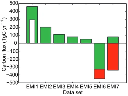
Table 6 presents terrestrial carbon fluxes for each LULUCF activity considered in the different LULUCF data sets. We note for this comparison that the total of LULUCF fluxes is only for the UNFCCC reporting countries. Thus the totals in Table 6 are slightly different from the global totals in Table 7 but the differences between the two values are much smaller than those between different data sets. Although 137 non-Annex I

coun-25

tries report total carbon fluxes, only 19 non-Annex I countries provide detailed carbon fluxes. Therefore, the total carbon fluxes for specific categories in EMI2 were

(20)

calcu-ACPD

8, 3843–3893, 2008

Full Screen / Esc

EGU

lated for the non-Annex I countries by scaling each country’s total fluxes by the ratios of the specific categories’ fluxes to the total for the 19 countries. EMI6 estimates a net sink of −465 TgC yr−1due to crop and pasture land conversions, while EMI7 shows the net emission of 474 TgC yr−1due to crop land conversion. In contrast to the other data sets, both EMI6 and EMI7 include the effects of environmental changes on fluxes of

5

carbon. Even though EMI6 and EMI7 consider different activities and their net fluxes are large and of opposite sign, the sums of their fluxes from all categories are in better agreement (i.e. −1393 and −958 TgC yr−1 _{for EMI6 and EMI7, respectively). These}

comparisons demonstrate the need to reconcile the different processes considered in different data sets.

10

Table 7 presents the change in carbon stocks (TgC yr−1_{) for EMI5, EMI6, and EMI7}

and the net carbon fluxes for EMI1, EMI3, and EMI4 for each pool considered in the different LUCF data sets in the 1990s. We note that carbon stock changes in a single pool are not necessarily equal to the emission or removal of CO₂from the atmosphere, because some carbon stock changes result from carbon transfers among pools rather

15

than exchanges with the atmosphere. Even though the total fluxes are in good agree-ment between EMI6 and EMI7, this does not indicate good agreeagree-ment, because the relative contributions of the VC, LIT, and SOC are significantly different between these data sets. These comparisons demonstrate the necessity of reconciling the different classifications of carbon pools used in the different data sets.

20

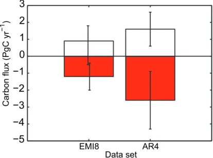
Figure 2 shows a comparison of the global consolidated LUCF flux and residual terrestrial sink (PgC yr−1) in the 1990s with the estimates from AR4 (Denman et al., 2007). The global flux for EMI8 was calculated by summing the consolidated esti-mates from the ten regions (i.e. those described by Houghton, 2003) that are rep-resented in all data sets. The EMI8 estimate of LUCF emissions (0.9 PgC yr−1) is

25

smaller than that from AR4 but within the uncertainty range given in that assessment (1.6±1.2 PgC yr−1) which was based on the higher values of Houghton (2003) and the lower of DeFries et al. (2002). The satellite estimate of carbon flux in the tropics due to LUC (0.95 Pg C yr−1) (Achard et al., 2002, 2004; DeFries et al., 2002) is significantly

(21)

ACPD

8, 3843–3893, 2008

Full Screen / Esc

EGU

smaller than the FAO-based estimate of 2.3 PgC yr−1 (Fearnside, 2000; Houghton, 2003). The EMI8 estimate of the global net terrestrial carbon flux (−0.4 PgC yr1) is also smaller than that given in the AR4 assessment but is within their uncertainty range (−1.0±0.6 PgC yr−1). This confirms that at the global level, our estimate is reason-able for further anaylsis, althouh this is not a validation of the consolidated estimate.

5

The AR4 estimate of the residual terrestrial sink (−2.6±1.7 TgC yr−1_{) is determined by}

subtraction of the LUC emissions from the net land-to-atmosphere flux estimated by inverse models and includes both climate feedback and CO2fertilization effects (which

are of order −1.2 PgC yr−1_{in EMI8), as well as nitrogen fertilization and other effects.}

3.4 Country analysis

10

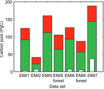
3.4.1 USA

A more detailed analysis is presented here for the USA. Figure 3 presents the sum of the terrestrial carbon pools (PgC) in the 1990s for EMI1, 2, 5, 6, and 7. Major differences are found in the LIT and SOC pools. The total soil organic matter is much smaller in the National inventory report to the UNFCCC (EMI2) than those in the other

15

estimates. The inventory data in EMI2 are reported only for the category of forest land remaining as forest land, while the other EMI estimates include non-forested lands. The different estimated amounts of SOC are partly due to the inclusion of non-forested lands. Guo et al. (2006) used the STATSGO database to estimate the SOC in the upper 1.0 m of the conterminous USA as in the USA report (EMI2) and restricted

20

their analysis to forested lands by overlaying the geo-referenced national land cover data (NLCD) based on 30 m resolution Landsat Thematic Mapper data acquired in the early 1990s with the STATSGO. In the NLCD, forestlands were divided into two parts: forested upland (228×104km2) and woody wetlands (21×104km2). The total forest area is in good agreement with the Forest Inventory Analysis (FIA) forest area used

25

in EMI2, but smaller than LUC3 (551×104km2) and LUC6 (338×104km2). The SOC value from EMI2 (15 PgC) is within the range for forested upland and woody wetlands

(22)

ACPD

8, 3843–3893, 2008

Full Screen / Esc

EGU

reported by Guo et al. (2006) (i.e. 8.5 to 42.5 PgC). The other model estimates are within the range from 25.4 to 113.1 PgC for total lands reported by Guo et al. (2006). EMI5 and EMI6 make separate estimates of the SOC pool for the forest carbon pools. Their contributions from non-forest lands (36 PgC for EMI6) partly offset the differences in the totals shown in Fig. 3. When Alaska is separated from the conterminous USA in

5

EMI6, the SOC in forests of the conterminous USA is calculated to be 39 PgC. EMI6 uses a potential vegetation map, so that the forest area in EMI6 is larger than the present-day FIA forest area. In addition, Guo et al. (2006) estimated an additional 2.3 to 16.4 PgC in the amount of SOC stored from 1.0 m to 2.0 m depth for forest and wetland. The SOC below 1.0 m may explain some of the differences in SOC between

10

EMI2 and EMI6. Consequently, SOC reported by EMI6 may be similar to that for EMI2 if comparison is restricted to the upper 1.0 m of soils in present-day forests within the conterminous USA. Although those from the other inventories are still large compared to EMI2, they should be compared for the same depth and forest area. Coarse woody debris (92% of LIT) is rather large in EMI7 and as large as woody tree parts (VC).

15

Harmon and Hua (1991) report that the ratio of CWD to live wood biomass is about 20–25% for subtropical, temperate, and boreal forests, which is consistent with EMI2.

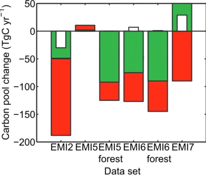
Figure 4 presents carbon stock changes for EMI2, EMI5, EMI6 and EMI7. The in-ventory data from EMI2 represent only forests including VC, LIT and SOC. The con-tributions of carbon stock changes for non-forests are insignificant for EMI6, because

20

woody invasions into grasslands are not considered in this model. However, signifi-cant differences in the carbon fluxes in forest lands and all lands are found for EMI5 mainly due to LUC emissions in cultivated areas and pasturelands. The averaged car-bon stock changes for forests show an accumulation of carcar-bon in LIT + SOC for EMI2 (−49 TgC yr−1), EMI5 (−92 TgC yr−1) and EMI6 (−90 TgC yr−1), as opposed to EMI7

25

which reports 51 TgC yr−1_{for all land cover types. Litter in EMI2 increases as the tree}

biomass increases, because estimates for dead wood are based on the ratio of downed dead wood to live tree biomass, while that in the process-based models does not in-crease linearly with tree biomass, but is determined by the models calculations, which

(23)

ACPD

8, 3843–3893, 2008

Full Screen / Esc

EGU

depend on the changes in climate (soil temperature and moisture).

Table 3 presents terrestrial carbon fluxes for each LUCF activity considered in the different LUCF data sets for the USA in the 1990s. We note that EMI4 represents the data of Hurtt et al. (2002) for this analysis in the USA. Only EMI1, EMI2 and EMI4 include the effects of fire suppression on LUCF fluxes, but EMI2 excludes woody

en-5

croachment in non-forests. The terrestrial carbon flux in EMI1 (−108 Tg C yr−1) is in good agreement with that of EMI6 excluding environmental factors (−114 TgC yr−1), but this agreement is fortuitous, because there is a large sink in EMI1 due to fire suppression (−130 TgC yr−1) which is not considered in EMI6. The overall fire sup-pression sink in EMI1 for the 1980s (−155 TgC yr−1) is in good agreement with that in

10

EMI4 (−150 TgC yr−1_{), but the fractions of VC and SOC could be different, because the}

changes in SOC associated with woody encroachment are assumed to be negligible in EMI1. When the comparison is restricted to forested lands, the UNFCCC reported carbon flux (−187 TgC yr−1_{) is in better agreement with that of EMI4 (−230 TgC yr}−1₎

but the difference is non-negligible. The sinks due to CO2 fertilization and climate

15

change predicted in EMI6 (−45 TgC yr−1) and EMI7 (−7 TgC yr−1) are relatively minor components, which is consistent with Caspersen et al. (2000) who used the FIA data to estimate the effects of environmental factors.

We compare inverse model fluxes for Temperate North America (TNA) (including the conterminous USA, most of Mexico, and southern Canada) with the bottom-up

20

inventories examined here for the USA, under the assumption that most of the esti-mated inverse flux would be associated with the USA. In Gurney et al. (2004) the net biospheric flux for TNA for 1992–1996 is −0.9 PgC yr−1, while more recent updates (Baker et al., 2006) give −1.1±0.23 PgC yr−1 _{for the decade 1991–2000. Depending}

on the use of all sites (i.e. ocean and land) versus only ocean observations, Patra et

25

al. (2006) estimated the TNA sink in the range from −0.56 to −0.69 PgC yr−1 for the 1999–2001 period. Based on many models’ inability to match observed CO₂profiles, Stephens et al. (2007) argue for 38% smaller uptake fluxes over northern lands but do not report values for TNA. These fluxes have the fossil-fuel and industrial sources

(24)

re-ACPD

8, 3843–3893, 2008

Full Screen / Esc

EGU

moved and represent the sum of changes due to LUCF and the environment (CO₂and nitrate fertilization, O3damage (Sitch et al., 2007), and climate). The decadal averaged

estimate for the total terrestrial uptake for TNA (Baker et al., 2006) is significantly larger than the sum of our consolidated estimate (−0.24 PgC yr−1 averaged over 1990–1999; EMI8) and other sinks such as carbon accumulated in sediments of reservoirs and

5

rivers and the balance of exports and imports by rivers and commerce (e.g. food and wood) (−0.08 to −0.17 PgC yr−1; Pacala et al., 2001). Examining this result together with the significant uncertainties in carbon pools and fluxes for non-forests (e.g. woody invasion) may imply that ENV factors (i.e. warming climate and fertilization) have played a larger role than estimated in EMI8.

10

3.4.2 Brazil

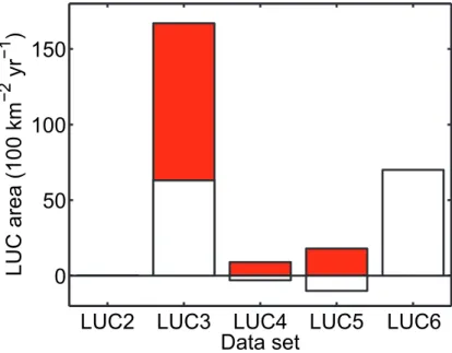
Figure 5 shows a comparison of the net LUC area changes in forests (102km2yr−1) due to conversion of forest to/from crop and pasture land in Brazil in 1990. Comparison of LUC3 and LUC6 both of which are based on SAGE for cropland conversions shows that the LUC3 net increase in forest areas (63×102km2yr−1) due to cropland

conver-15

sion is consistent with that in LUC6 (70×102km2yr−1). However, the sum of the gross decrease in forest and grassland areas in LUC3 (−29×102km2yr1) due to conversion of forest to crop and pasture land is smaller than that in LUC6 (−34×102km2yr−1_{) from}

1989 to 1990 in Brazil. The difference is mainly due to the simple interpolation to T42 in the case of LUC3, because the estimate was −34×102km2yr−1on the original grid.

20

Further, the gross decrease in forests in LUC3 (−28×102km2yr−1_{) due to crop and}

pasture land conversions is larger than that in LUC6 (−8×102km2yr−1) due to crop land conversion from 1989 to 1990 in Brazil. Therefore, LUC3 accounts for major de-forestation due to LUC, as opposed to LUC6. As a result, the net change due to LUC in Fig. 5 is similar but the gross deforestation is different. Regarding the conversion

25

of natural forests to cropland, there are two reasons that could cause differences be-tween the data sets: (1) the satellite based classifications used for the present-day natural vegetation cover versus classification based on ground observations and (2)

(25)

ACPD

8, 3843–3893, 2008

Full Screen / Esc

EGU

the use of fractional natural plant functional types (PFTs) versus a single land-use type approach for each grid area. The first factor determines what types of natural vegeta-tion were assumed to exist on the Earth’s surface (e.g. forests, grasses or bare land), which could vary between different data sources. In LUC6, the GLC2000 data set was combined with 1992 satellite data, and the grid cells were adjusted to have the same

5

fractions of tree covered land, bare ground and inland water as in GLC2000 and to have the same cropland and grassland fractions as in 1992. In the biogeochemical models (EMI6 and EMI7), forest grid cells may include non-forest areas, but they are treated as forests. LUC3 uses the simplified vegetation map from the Matthews (1983) global ecosystem data set. Moreover, these data are significantly different from those

10

reported by LUC5 which includes secondary forest based on SAGE and other sources, mainly because LUC5 used a linear interpolation between 1970 and 1990, while other data sets used a database based on a single year. As opposed to LUC5, the LUC3 and LUC6 data sets did not track LUC activities, and therefore they represent a “net” change of areas associated with tree PFTs that were converted to cropland area, i.e.

15

the primary (or secondary) forest area that was converted to crops, minus any crop (and pasture) area converted back to secondary forest. Areas converted from crop and pasture could include both active human conversions (e.g. short-rotation forestry in Brazil) and the passive reversion of abandoned crop or pasture land to “natural” (but possibly degraded) forest. The errors implicit in this approach might have significant

20

impacts on carbon dynamics resulting from the changes in land cover at small spa-tial scales and shorter term durations. LUC2 and LUC4 show small net changes in LUC areas. LUC4 in the 1990s presents substantial gross changes of deforestation (−73×102km2yr−1) and AR (79×102km2yr1), while LUC2 assigned all the changes in cropland areas to non-forest conversions and thus has a zero net change in forest

25

areas. Even though LUC2, LUC4 and LUC5 use the FAOSTAT for crop and pasture lands, the net forest area changes in LUC2 (zero), LUC4 (6×102km2yr−1), and LUC5 (7×102km2yr−1) in the 1990s are substantially smaller than that for 1990–2000

(26)

re-ACPD

8, 3843–3893, 2008

Full Screen / Esc

EGU

ported by FAO (2006) (−268×102km2yr−1). According to Ara ´ujo et al. (20073), the allocations of deforestated areas due to pasture and agriculture expansions in HYDE used by de Campos et al. (2005) do not match those in INPE, primarily due to dif-ferences between the HYDE and INPE databases in the basic methodology and the concept of deforestation. These comparisons demonstrate the need to constrain the

5

rate of conversions of natural forest areas in each specific LUC activity for the calcula-tion of LUC.

Figure 6 presents terrestrial carbon fluxes (TgC yr−1) for each LUCF activity consid-ered in the different emission data sets for Brazil in the 1990s. EMI1 shows a ma-jor source of carbon fluxes to the atmosphere due to forest conversion to pasture.

10

Carbon fluxes due to land conversions are opposite in sign for Brazil between EMI6 (−327 TgC yr−1_{) and EMI7 (79 TgC yr}−1_{). The SAGE data show high-clearing rates in}

eastern Brazil during 1960 – 1980 and extensive cropland abandonment during 1980– 1992 except for southeastern Brazil. When the comparison is restricted to the early 1990s, because different secondary assumptions are used for land cover changes in

15

the 1990s, EMI6 indicates a 500 (TgC yr−1) sink due to LUC, while EMI7 shows exten-sive emissions due to conversion of forest to cropland during the same period. This might be partly due to the inclusion of pasture land conversion, because the net forest area change (104×102km2) due to pasture conversion is larger than that due to crops in LUC3 (Fig. 5). Since FAO (2006) reports a decrease in forest areas in Brazil between

20

1990 and 2000, the positive sign (i.e. net source) in EMI7 is consistent with EMI1. The emissions in inventory approaches (EMI2, EMI3, and EMI4) are not directly compara-ble to the other emissions shown in Fig. 6, because there is a time delay in emissions into the atmosphere that are accounted for only in EMI1, EMI5, EMI6 and EMI7. The annual gross emission due to deforestation in EMI2 can be compared with that in EMI3,

25

as follows. If we assume that 100% of the above-ground biomass in EMI3 is

immedi-3

Ara ´ujo, M. S. M., Silva, C., and Campos, C. P.: Land use change sector contribution to the carbon historical emissions and the sustainability case study of the Brazilian Legal Amazon, Renewable Sustainable Rev., accepted, 2007.

(27)

ACPD

8, 3843–3893, 2008

Full Screen / Esc

EGU

ately removed from the forest as in EMI2, the gross emissions due to deforestation are in better agreement between EMI2 (251 TgC yr−1_{) and EMI3 (222 TgC yr}−1_{) as well}

as the deforestation area between the INPE report (−313×102km2yr−1) from 1988 to 1994 and that from FAO (1993) (−367×102km2yr−1) from 1981 to 1990. EMI2 does not account for the fate of the carbon removed from the forests. If we assume that

5

the carbon is either emitted to the atmosphere or harvested, combining the emissions to the atmosphere in EMI3 (111 TgC yr−1) and the harvested wood including slash in EMI4 (79 TgC yr−1_{) yields a smaller gross emission due to deforestation than that in}

EMI2 (251 TgC yr−1). However, Asner et al. (2005) reported that selectively logged ar-eas ranged from 121 to 198 (×102km2yr−1) between 1999 and 2002, equivalent to 60

10

to 123% of the deforestation area reported by INPE. This may suggest that selective logging has been implicitly taken into account in the net emissions since the selective logging area could have been deforested or regenerated between the years 1988 and 1994 when satellite estimates were possible. In Brazil, climate and CO₂responses are significantly different between EMI6 and EMI7, whereas they were insignificant in the

15

USA.

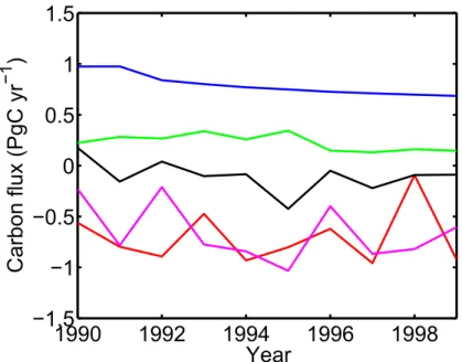
We can compare the available inverse model fluxes for Tropical (1.07±0.69 PgC yr−1₎

and South America (−0.64 ±0.51 PgC yr−1) from Baker et al. (2006) with our con-solidated bottom-up method for the decade 1991 – 2000. The total emission for Latin America in EMI8 (−0.17 PgC yr−1_{) is smaller than that from the inverse}

mod-20

els (0.43±0.86 PgC yr−1) but within the uncertainty range. The interannual variability of CO2 flux in EMI8 for Latin America (Fig. 7) is significantly smaller than the inverse

estimates (Baker et al., 2006). The bottom-up estimates of LUCF may capture the averaged changes of the net LUCF emissions but may not fully account for the timing of CO2 flux changes. Further, there are significant uncertainties in selective logging

25

(e.g. Nepstad et al., 1999; Asner et al., 2005) and open vegetation burning (e.g. van der Werd et al., 2004; Jain et al., 2006; Ito et al., 2007b). This may imply that accurate estimates of the short-term flux would play a key role in closing the gap between the bottom-up and top-down estimates.

(28)

ACPD

8, 3843–3893, 2008

Full Screen / Esc

EGU

4 Summary and conclusions

There are large differences in the processes included in different LUCF data sets at the global level. Thus, model estimates for LUCF emissions without climate feed-back range from −0.5 to 1.4 PgC yr−1. The Houghton et al. (2006) emissions are the highest of these emissions but this data set includes the most complete set of LUCF

5

processes. We constructed a consolidated estimate of global LULUCF fluxes from dif-ferent processes which used the Houghton et al. (2006) estimates if not included in the other models and an average of the estimates for each process when indepen-dent data sets were available. This yields a global estimate for LUCF emissions of 0.9 PgC yr1 for the 1990s. The global estimate of LUCF emissions in the consolidated

10

estimate (i.e. 0.9 with a range from –0.6 to 1.8 Pg yr−1) is consistent with AR4 as-sessment (1.6±1.2 PgC yr−1). Overall, climate feedback and fertilization effects could significantly decrease the net global emissions from LUCF, but more research will be needed to better quantify these effects. Climate feedback and fertilization effects in the 2 biogeochemical cycle models reviewed here lead to a C sink ranging from −0.9

15

to −1.4 Pg yr−1_{, which is smaller than that of the AR4 estimate of the residual}

terres-trial sink but within their uncertainty range (−2.6±1.7 TgC yr−1). The AR4 estimate may include nitrogen fertilization and other effects that are not in the 2 biogeochemical mod-els. Our consolidated estimate of the net global terrestrial carbon flux (i.e. the sum of emissions and uptake, −0.4 PgC yr−1) is also smaller than that of the AR4 assessment,

20

but still just within the uncertainty range derived from a combination of inverse models and observations (−1.0±0.6 PgC yr−1_).

Estimates of LULUCF emissions from the UNFCCC that are nearly global in scope are −0.25 PgC yr−1. The UNFCCC guidelines suggest that this estimate should in-clude all processes as does our consolidated estimate. However, these two estimates

25

are not always comparable. In order to investigate the possible reasons for the large differences between the different estimates, we investigated two specific countries. For example, our consolated estimate includes carbon fluxes in non-forested areas