HAL Id: hal-03215525
https://hal.archives-ouvertes.fr/hal-03215525
Submitted on 3 May 2021
HAL is a multi-disciplinary open access
archive for the deposit and dissemination of
sci-entific research documents, whether they are
pub-lished or not. The documents may come from
teaching and research institutions in France or
abroad, or from public or private research centers.
L’archive ouverte pluridisciplinaire HAL, est
destinée au dépôt et à la diffusion de documents
scientifiques de niveau recherche, publiés ou non,
émanant des établissements d’enseignement et de
recherche français ou étrangers, des laboratoires
publics ou privés.
seasonal amplitude increase of carbon fluxes in
terrestrial ecosystems: a multimodel analysis
Fang Zhao, Ning Zeng, Ghassem Asrar, Pierre Friedlingstein, Akihiko Ito,
Atul Jain, Eugenia Kalnay, Etsushi Kato, Charles Koven, Ben Poulter, et al.
To cite this version:
Fang Zhao, Ning Zeng, Ghassem Asrar, Pierre Friedlingstein, Akihiko Ito, et al.. Role of CO2, climate
and land use in regulating the seasonal amplitude increase of carbon fluxes in terrestrial ecosystems:
a multimodel analysis. Biogeosciences, European Geosciences Union, 2016, 13 (17), pp.5121-5137.
�10.5194/bg-13-5121-2016�. �hal-03215525�
www.biogeosciences.net/13/5121/2016/ doi:10.5194/bg-13-5121-2016
© Author(s) 2016. CC Attribution 3.0 License.
Role of CO
2
, climate and land use in regulating the seasonal
amplitude increase of carbon fluxes in terrestrial
ecosystems: a multimodel analysis
Fang Zhao1,2, Ning Zeng1,3, Ghassem Asrar4, Pierre Friedlingstein5, Akihiko Ito7, Atul Jain8, Eugenia Kalnay1, Etsushi Kato9, Charles D. Koven10, Ben Poulter11, Rashid Rafique4, Stephen Sitch6, Shijie Shu8, Beni Stocker12, Nicolas Viovy13, Andy Wiltshire14, and Sonke Zaehle15
1Department of Atmospheric and Oceanic Science, University of Maryland, College Park, MD 20742, USA 2Potsdam Institute for Climate Impact Research, Telegraphenberg, 14412 Potsdam, Germany
3Earth System Science Interdisciplinary Center, University of Maryland, College Park, MD 20742, USA 4Joint Global Change Research Institute, Pacific Northwest National Laboratory, College Park, MD 20742, USA 5University of Exeter, College of Engineering Mathematics and Physical Sciences, Exeter, EX4 4QF, UK 6University of Exeter, College of Life and Environmental Sciences, Exeter, EX4 4QF, UK
7Center for Global Environmental Research, National Institute for Environmental Studies, 305-0053 Tsukuba, Japan 8Department of Atmospheric Sciences, University of Illinois, Urbana, IL 61801, USA
9Global Environment Program Research & Development Division, the Institute of Applied Energy (IAE), 105-0003 Tokyo,
Japan
10Earth Sciences Division, Lawrence Berkeley National Laboratory, Berkeley, CA 94720, USA
11Institute on Ecosystems and Department of Ecology, Montana State University, Bozeman, MT 59717, USA 12Climate and Environmental Physics, Physics Institute, University of Bern, 3012 Bern, Switzerland
13Laboratoire des Sciences du Climat et de l’Environnement, CEA CNRS UVSQ, 91191 Gif-sur-Yvette, France 14Hadley Centre, Met Office, Exeter, EX1 3PB, UK
15Biogeochemical Integration Department, Max Planck Institute for Biogeochemistry, P.O. Box 10 01 64,
07701 Jena, Germany
Correspondence to:Fang Zhao (fangzhao@pik-potsdam.de)
Received: 4 April 2016 – Published in Biogeosciences Discuss.: 11 April 2016
Revised: 22 August 2016 – Accepted: 24 August 2016 – Published: 14 September 2016
Abstract. We examined the net terrestrial carbon flux to the atmosphere (FTA) simulated by nine models from the
TRENDY dynamic global vegetation model project for its seasonal cycle and amplitude trend during 1961–2012. While some models exhibit similar phase and amplitude compared to atmospheric inversions, with spring drawdown and au-tumn rebound, others tend to rebound early in summer. The model ensemble mean underestimates the magnitude of the seasonal cycle by 40 % compared to atmospheric inversions. Global FTA amplitude increase (19 ± 8 %) and its decadal
variability from the model ensemble are generally consis-tent with constraints from surface atmosphere observations. However, models disagree on attribution of this long-term
amplitude increase, with factorial experiments attributing 83 ± 56 %, −3 ± 74 and 20 ± 30 % to rising CO2, climate
change and land use/cover change, respectively. Seven out of the nine models suggest that CO2fertilization is the strongest
control – with the notable exception of VEGAS, which at-tributes approximately equally to the three factors. Generally, all models display an enhanced seasonality over the boreal region in response to high-latitude warming, but a negative climate contribution from part of the Northern Hemisphere temperate region, and the net result is a divergence over cli-mate change effect. Six of the nine models show that land use/cover change amplifies the seasonal cycle of global FTA:
crop expansion or agricultural intensification, as revealed by their divergent spatial patterns. We also discovered a moder-ate cross-model correlation between FTAamplitude increase
and increase in land carbon sink (R2=0.61). Our results suggest that models can show similar results in some bench-marks with different underlying mechanisms; therefore, the spatial traits of CO2 fertilization, climate change and land
use/cover changes are crucial in determining the right mech-anisms in seasonal carbon cycle change as well as mean sink change.
1 Introduction
The amplitude of the atmospheric CO2 seasonal cycle is
largely controlled by vegetation growth and decay in the Northern Hemisphere (NH) (Bacastow et al., 1985; Graven et al., 2013; Hall et al., 1975; Heimann et al., 1998; Pearman and Hyson, 1980; Randerson et al., 1997). Since 1958,
at-mospheric CO2measurements at Mauna Loa, Hawai’i, have
tracked a 15 % rise in the peak-to-trough amplitude of the detrended CO2 seasonal cycle (Zeng et al., 2014),
suggest-ing an enhanced ecosystem activity due to changes in the strength of the ecosystem’s production and respiration and to a shift in the timing of their phases (Randerson et al., 1997). In addition, some evidence suggests a latitudinal gra-dient in CO2amplitude increase in the NH, with a larger
in-crease at Pt. Barrow, Alaska (0.6 % yr−1)than at Mauna Loa (0.32 % yr−1)(Graven et al., 2013; Randerson et al., 1999). Previous studies have attempted to attribute the long-term CO2amplitude increase to stimulated vegetation growth
un-der rising CO2and increasing nitrogen deposition (Bacastow
et al., 1985; Reich and Hobbie, 2013; Sillen and Dieleman, 2012). Another possible explanation offered is the effect of a warmer climate, especially in boreal and temperate regions, on the lengthening of growing season, enhanced plant growth (Keeling et al., 1996; Keenan et al., 2014), vegetation phenol-ogy (Thompson, 2011), ecosystem composition and struc-ture (Graven et al., 2013). The agricultural green revolution, due to widespread irrigation, increasing management inten-sity and high-yield crop selection, could also contribute to the dynamics of the CO2seasonal amplitude (Zeng et al., 2014;
Gray et al., 2014). Even though these studies are helpful in understanding the role of CO2, climate and land use/cover
changes, detailed knowledge of the relative contribution of these factors is still lacking.
Dynamic vegetation models are useful tools not only to disentangle effects of various mechanisms but also to offer insights on how terrestrial ecosystems respond to external changes. Attribution of the role of CO2, climate and land
use has been attempted with a single model (Zeng et al., 2014), but comprehensive multimodel assessment efforts are still missing. Two important questions must be addressed in such efforts, namely, whether the models can simulate
ob-served CO2amplitude increase, and to what extent their
fac-torial attributions agree. For the first question, the Coupled Model Intercomparison Project Phase 5 (CMIP5) Earth Sys-tem Models seem to be able to simulate the amplitude in-crease measured at the Mauna Loa and Point Barrow surface stations (Zhao and Zeng, 2014); however, they underestimate the amplitude increase compared to upper air (3–6 km) obser-vations significantly (Graven et al., 2013). It is possible that uncertainty in vertical mixing in atmospheric transport mod-els (Yang et al., 2007), instead of biases in dynamic vege-tation models themselves, causes the severe underestimation of upper air CO2 amplitude increase. For the second
ques-tion, in a unique modeling study conducted by McGuire et al. (2001), both CO2fertilization and land use/cover changes
were found to contribute to CO2amplitude increase at Mauna
Loa, but the four models disagreed on the role of climate and the relative importance of the factors they studied. Since then, no published study has explored the reliability of mod-els’ simulation of seasonal carbon cycle and quantified the relative contribution of various factors affecting it.
An important trait of the three main factors (i.e., CO2,
cli-mate and land use/cover change) we consider in this study is their different regional influence. Rising CO2 would likely
enhance productivity in all ecosystems. Climate warming may affect high-latitude ecosystems more than tropical and subtropical vegetation, and droughts would severely affect plant growth in water-limited regions. Similarly, the effect of land use/cover change may be largely confined to agricultural fields and places with land conversion, mostly in midlatitude regions. Because of their different spatial traits, it is possible to determine which factor is most important with strategi-cally placed observations. Forkel et al. (2016) recently de-rived a latitudinal gradient of CO2amplitude increase based
on CO2observational data, which would provide strong
sup-port that high-latitude warming is the most imsup-portant factor. However, with only two sites north of 60◦N, the robustness of the result is limited. In lieu of additional observational ev-idence, as a first step, it is necessary to investigate how the models represent the regional patterns of seasonal change of carbon flux.
A number of recent studies have addressed different as-pects of the seasonal amplitude topic. For example, the latitu-dinal gradient of CO2seasonal amplitude was used as
bench-mark in assessing the performance of JSBACH model (Dal-monech and Zaehle, 2013; Dal(Dal-monech et al., 2015). Based on a model intercomparison project – Multiscale Synthe-sis and Terrestrial Model Intercomparison Project (MsTMIP; Huntzinger et al., 2013; Wei et al., 2014) – Ito et al. (2016) focused on examining the relative contribution of CO2,
cli-mate and land use/cover changes, but little model evaluation was performed. In order to further explore and understand the seasonal fluctuation of carbon fluxes, a more comprehensive study including both the model evaluation and factorial anal-ysis is needed. The TRENDY model intercomparison project provides a nice platform for such analysis (Sitch et al., 2015).
Site-level model–data comparison of seasonal carbon fluxes has been performed extensively in Peng et al. (2015) for the first synthesis of TRENDY models. Using both the second synthesis of TRENDY models simulations and observations, in this study we aim to achieve two main goals. (1) Assess how well the models simulate the climatological seasonal cy-cle and seasonal amplitude change of the carbon flux against a number of observational-based datasets (CO2observations
and atmospheric inversions). (2) Analyze the relative con-tribution from the three main factors (CO2fertilization,
cli-mate and land use/cover change) to the seasonal amplitude increase, both at the global and regional level.
2 Method
2.1 Terrestrial ecosystem models and TRENDY
experiment design
Monthly net biosphere production (NBP) simulations for 1961–2012 from nine TRENDY models participating in the Global Carbon Project (Le Quéré et al., 2014) were examined (Table 1). A set of three offline experiments driven by either constant or varying climate data and other input such as at-mospheric CO2and land use/cover forcing were designed in
the TRENDY project to differentiate the role of CO2, climate
and land use (Table 2). We primarily evaluated results from the S3 experiment, where the models are driven by time-varying forcing data (Appendix A). In addition, we also used results from the S1 and S2 experiments.
2.2 Observations and observational-based estimates
In light of the large difference in the Coupled Climate Car-bon Cycle Model Intercomparison Project (C4MIP) models’ sensitivity to CO2change (Friedlingstein et al., 2013), it is
essential to evaluate whether the terrestrial biosphere models are able to capture important features of CO2seasonal cycle.
The scarcity of observational constraints, especially the lack of long-term continuous observational records, limits our ca-pacity to fully evaluate the dynamic processes in terrestrial ecosystem models. Nevertheless, in this study we make a first-order approximation of the evolution of the global CO2
seasonal cycle, using limited CO2observation data.
Follow-ing Zeng et al. (2014), monthly Mauna Loa records from 1961 to 2012 and a global monthly CO2index for the period
of 1981–2012 were retrieved from NOAA’s Earth System Research Laboratory (ESRL; www.esrl.noaa.gov/gmd/ccgg/ trends/). Details on the data processing, choice of stations and quality control procedures in deriving the global CO2
in-dex (globally averaged CO2concentration) can be found in
Thoning et al. (1989) and Masarie and Tans (1995).
Fluxes from process-based models can be directly com-pared with monthly gridded fluxes from atmospheric
inver-sions, which combine measured atmospheric CO2
concen-tration at multiple sites across the globe with atmospheric
transport driven by meteorological data. Two representative inversions, Jena (Jena81 and Jena99, Rödenbeck et al., 2003) and the CarbonTracker (Peters et al., 2007), are included for comparison (Appendix B). For an exhaustive intercompari-son of the atmospheric inversions, please refer to Peylin et al. (2013).
2.3 Calculating the seasonal cycle and its amplitude change
All monthly NBP- and inversion-derived fluxes are first re-sampled (box averaging, conserving mass) to a uniform 0.5◦×0.5◦ global grid in units of kg C m−2yr−1. For the TRENDY model simulations, we further define net carbon flux from the land to the atmosphere (FTA), which simply
reverses the sign of NBP, so that positive FTA indicates net
carbon release to the atmosphere, and negative FTAindicates
net carbon uptake. FTA represents the sum of residual land
sink and land use emission, including fluxes from ecosys-tem production and respiration, fire, harvest, etc.; although some models may not simulate all the processes. Changes in global atmospheric CO2concentration are then equal to
FTAplus ocean–atmosphere flux and fossil fuel emission. For
inversion-derived fluxes, only terrestrial ecosystem fluxes are used (optimized global biosphere fluxes plus fire fluxes in CarbonTracker), which are conceptually similar to FTA,
except that atmospheric transport is included. Atmospheric transport can significantly affect local carbon fluxes (Ran-derson et al., 1997); however, the impact is limited on global and large zonal band totals.
The seasonal amplitudes of Mauna Loa Observatory CO2
growth rate, global CO2growth rate and fluxes from model
simulations and inversions are processed with a curve fitting package called CCGCRV from NOAA/ESRL (http://www. esrl.noaa.gov/gmd/ccgg/mbl/crvfit/crvfit.html). This pack-age first filtered out the high-frequency signals with a series of internal steps involving polynomial and harmonic fitting, detrending and band-pass filtering, and then the amplitude is defined as the difference between each year’s maximum and minimum. For the latitudinal plots only, we simply use maxi-mum and minimaxi-mum of each year to define the seasonal ampli-tude without first filtering the data. Previous studies (Graven et al., 2013; Randerson et al., 1997) have established that FTA
accounts for most of seasonal amplitude change from atmo-spheric CO2, and the Mauna Loa CO2record is considered
to represent the evolution of global mean CO2well
(Kamin-ski et al., 1996). Therefore, similar to our earlier work (Zeng et al., 2014), we evaluated the amplitude change of modeled FTAwith Mauna Loa CO2, ESRL’s global CO2and the
atmo-spheric inversions, to assess whether the models are able to capture both the global trend and latitudinal patterns. For rel-ative amplitude changes, we compute the multimodel ensem-ble mean after deriving the time series (relative to their 1961– 1970 mean) from individual model simulations, so that mod-els with large amplitude change would not have a huge
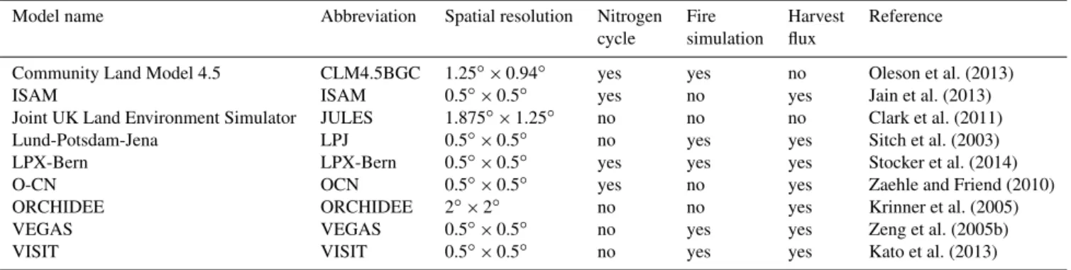
ef-Table 1. Basic information for the nine TRENDY models used in this study.
Model name Abbreviation Spatial resolution Nitrogen Fire Harvest Reference
cycle simulation flux
Community Land Model 4.5 CLM4.5BGC 1.25◦×0.94◦ yes yes no Oleson et al. (2013)
ISAM ISAM 0.5◦×0.5◦ yes no yes Jain et al. (2013)
Joint UK Land Environment Simulator JULES 1.875◦×1.25◦ no no no Clark et al. (2011)
Lund-Potsdam-Jena LPJ 0.5◦×0.5◦ no yes yes Sitch et al. (2003)
LPX-Bern LPX-Bern 0.5◦×0.5◦ yes yes yes Stocker et al. (2014)
O-CN OCN 0.5◦×0.5◦ yes no yes Zaehle and Friend (2010)
ORCHIDEE ORCHIDEE 2◦×2◦ no no yes Krinner et al. (2005)
VEGAS VEGAS 0.5◦×0.5◦ no yes yes Zeng et al. (2005b)
VISIT VISIT 0.5◦×0.5◦ no yes yes Kato et al. (2013)
fect on the ensemble mean. Additionally, global and regional mean seasonal cycles over 2001–2010 between the models and inversions are compared. We further compared the sea-sonal amplitude of zonally averaged FTAfrom TRENDY and
atmospheric inversions. To smooth out minor variations but ensure similar phase in aggregation, we first resampled FTA
into 2.5◦resolution, then summed it over latitude bands for the 2001–2010 mean FTAseasonal cycle.
2.4 Factorial analyses
Relative amplitudes for 1961–2012 (relative to 1961–1970 mean seasonal amplitude) from the experiments S1, S2 and S3, respectively, are calculated using the CCGCRV pack-age for each model, and a linear trend (in % yr−1) is de-termined for that period. We use relative amplitude for per-centage change to minimize impacts of some differing im-plementation choices like climate data in S1 (CO2)among
the models. The effect of CO2 on the relative amplitude
change is represented by a trend of S1 (CO2only) results; the
S2 (CO2+climate) results show a trend that is the sum of
CO2 and climate effects, and the S3 (CO2+climate + land
use/cover) simulations include trends from time-varying CO2, climate and land use/cover change (abbreviated as land
use for text and figures). For simplicity, the effect of “cli-mate” as used in this paper includes the synergy of CO2and
climate, and similarly the effect of “land use/cover” also in-cludes the synergy terms. Therefore, the effects of CO2,
cli-mate and land use/cover are then quantified as the trend for S1, the trend of S2 minus the S1 trend and the trend of S3 minus the S2 trend, respectively. Note that the synergy terms are likely small in some of the current generation dynamic vegetation models, such as those shown in previous sensitiv-ity experiment results (Zeng et al., 2014).
2.5 Spatial attribution
Spatial attribution of global FTA amplitude change can be
difficult due to the phase difference at various latitudes. For example, the two amplitude peaks at northern and southern subtropics caused by monsoon movements are largely out of
phase, and the net contribution to global FTA amplitude
in-crease after their cancelation is small (Zeng et al., 2014). To quantify latitudinal and spatial contributions for each model, a unique quantity – Fki
A – the difference between the
max-imum month (i_max) and the minmax-imum month (i_min) of model i’s global FTA, based on model i’s 2001–2010 mean
seasonal cycle is defined as Eq. (1): Fki A=F i kA(i_max)−F i kA(i_min). (1)
The subscript k denotes the index of each latitudinal band or spatial grid, and A is the index of the year, ranging from 1961 to 2012. Fki
A could be quite different for each model:
for VEGAS, Fki
A is FTA in November (i_max = 11) minus
FTA in July (i_min = 7) in year A, and for LPJ, FkiAis FTA
in March (i_max = 3) minus FTAin June (i_min = 6) in year
A. The indexes i_max and i_min are fixed for each model, as summarized in Table 3. For all three experiments, Fki
Ais
computed each year in 1961–2012 and at every latitude band or spatial grid (k), and then the trends of Fki
Aare calculated.
The spatial aggregation of the resulted latitudinal-dependent trends would then approximately be equal to the trend of
global FTAmaximum-minus-minimum seasonal amplitude.
3 Results
3.1 Mean seasonal cycle of FTA
Four of the nine models (CLM4.5BGC, LPX-Bern,
OR-CHIDEE and VEGAS) simulate a mean global FTA
sea-sonal cycle of similar amplitude and phase compared with the Jena99 and CarbonTracker inversions (Fig. 1, Table 3). The other five models have much smaller seasonal amplitude than inversions, and the shape of the seasonal cycle is also notably different. As a result, the models’ ensemble global FTAhas seasonal amplitude of 26.1 Pg C yr−1during 2001–
2010, about 40 % smaller than the inversions (Fig. 4 inset,
Table 3). The model ensemble annual mean FTA (residual
land sink plus land use emission) is −1.1 Pg C yr−1for 2001– 2010, 30 % smaller than the inversions (Table 3). In some
models (ISAM, JULES and LPJ for the northern temper-ature region in Fig. 2) FTA rebounds back quickly,
result-ing in a late summer FTA maximum. The midsummer
re-bound is unlikely a model response to pronounced seasonal drought after 2000, as it is persistent in the mean seasonal cycle over every decade since 1961. A probable cause is the strong exponential response of soil respiration to temperature increase, which may lead to heterotopic respiration higher than net primary production (NPP) in summer. For example, HadGEM2-ES and HadCM3LC, which employ a forerunner of JULES3.2 used in this study, are found to have a com-paratively better simulation of the seasonal cycle (Collins et al., 2011), due to a combination of a more sensitive temper-ature rate modifier combined with a larger seasonal soil tem-perature that is used in the later version of JULES. Alexan-drov (2014) shows that both the amplitude underestimation and phase shift of FTAseasonal cycle can be improved by
in-creasing water use efficiency, dein-creasing temperature depen-dence of heterotrophic respiration and increasing the share of quickly decaying litterfall. Another probable factor is the simulation of plant phenology. With the help of remote sens-ing data, better phenology in model simulation has been shown to improve seasonal cycle simulation of carbon flux (Forkel et al., 2014). Additionally, the effect of carbon re-lease from crop harvest is considered. If harvested carbon is the main cause for the midsummer rebound in some mod-els, the rebound should be much less pronounced for the S2 (constant 1860 land use/cover) experiment, given that crop-land area in 1860 is less than half of the 2000 level. However, based on the comparison between the S2 and S3 experiments over the global and northern temperate (major crop belts) FTA seasonal cycle (Figs. S1 and S2 in the Supplement),
the impact of harvested carbon flux is unlikely to explain the midsummer rebound. This is probably due to modeling efforts to prevent the sudden release of harvested carbon. In-stead, carbon release of harvested products and/or their resid-uals is usually either spread over 12 months (i.e., LPJ, LPX-Bern, OCN, ORCHIDEE), or it enters soil litter carbon pool (i.e., ISAM) for subsequent decomposition over time.
TRENDY models and inversions agree best over the boreal region (Fig. 2a). While underestimating the global seasonal cycle, LPJ and VISIT both simulate similar boreal FTA
am-plitude as inversions. In addition to ORCHIDEE and
VEGAS, LPJ and LPX-Bern also simulate maximum CO2
drawdown in July for the boreal region, same as the inver-sions, while the other five models have the FTAminimum in
June. Large model spread is present for the northern temper-ate region, especially in summer. Both inversions and models agree marginally over the phase of the FTAseasonal cycle in
the tropics. The northern and southern tropics show seasonal cycles that are largely out of phase except for LPJ (Fig. 2c, d), due to the seasonal movement of the tropical rain belt in the intertropical convergence zone (ITCZ). The southern ex-tratropics exhibit even smaller FTAamplitude due to the
rel-atively small biomass of the southern extratropics, and most
PgC yr
–1
Figure 1. Mean seasonal cycle of global net carbon flux from nine TRENDY models (S3 experiment) and two inversions, Jena99 and CarbonTracker, averaged over 2001–2010.
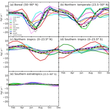
(23.5–50° N) (0–23.5° S) (0–23.5° N) (50–90° N) (23.5–90° S) PgC yr –1 PgC yr –1 PgC yr –1
Figure 2. Mean seasonal cycle of net carbon flux totals over bo-real (50–90◦N), northern temperate (23.5–50◦N), northern tropics (0–23.5◦N), southern tropics (0–23.5◦S) and southern extratrop-ics (23.5–90◦S) from nine TRENDY models and two inversions, Jena99 and CarbonTracker, averaged over 2001–2010.
models and inversions indicate a maximum FTAaround July,
opposite in phase to its NH counterpart.
The latitudinal pattern of the multimodel median FTA
am-plitude is remarkably similar to the inversions (Fig. 3). A notable feature is the large seasonality over the NH midlat-itude to high-latmidlat-itude region driven by temperature contrast between winter and summer. The model median also
cap-Table 2. Experimental design of TRENDY simulations.
Name Time period Atmospheric CO2 Climate forcing Land-use history∗∗
S1 1901–2012 Time-varying Constant∗ Constant (1860)
S2 Time-varying
S3 Time-varying
∗Constant climate state is achieved by repeated or randomized or fixed climate cycles depending on each model. ∗∗Only the crop, pasture and wood harvest information is included, so land use in this study refers specifically to
the related agricultural and forestry processes.
Table 3. Global mean net land carbon flux, seasonal amplitude, the maximum and minimum months of FTAfor the nine TRENDY models and their ensemble mean during 1961–1970 and 2001–2010 periods. For the later period, characteristics of the atmosphere inversions Jena99 and CarbonTracker are also listed.
Name Net carbon flux Seasonal amplitude FTA FTA
(Pg C yr−1) (Pg C yr−1) minimum maximum 1961–1970 2001–2010 1961–1970 2001–2010 2001–2010 2001–2010 CLM4.5BGC 0.1 −2.4 38.4 44.3 Jun Nov
ISAM 0.7 0.0 17.6 19.1 Jun Oct
JULES −0.2 −1.7 15.1 19.0 May Aug LPJ 1.3 −0.6 18.6 23.4 Jun Mar LPX-Bern 0.6 0.0 33.0 37.9 Jun Jan OCN 0.9 −1.8 16.1 21.6 Jun Nov ORCHIDEE 0.1 −0.7 35.7 39.9 Jul Mar VEGAS −0.4 −1.5 40.7 46.7 Jul Nov VISIT 0.2 −1.4 25.3 28.9 Jun Nov Ensemble 0.4 −1.1 22.4 26.1 Jun Nov
Jena99 −1.7 46.8 Jul Oct
CarbonTracker −1.6 39.9 Jul Nov
PgC yr
–1
m
° S ° S ° S ° S ° N ° N ° N ° N ° N ° N ° N
m
Figure 3. Latitudinal dependence of the seasonal amplitude of land–atmosphere carbon flux from the TRENDY multimodel me-dian (red line, and the pink shading indicates the 10 to 90 per-centile range of model spread), two atmospheric CO2inversions,
Jena99 (black dashed line) and CarbonTracker (gray dashed line), and each individual model (thin line). Fluxes are first resampled to 2.5◦×2.5◦, then summed over each 2.5◦latitude band (Pg C yr−1 per 2.5◦latitude) for the TRENDY ensemble and inversions.
tures the two subtropical maxima around 10◦N and 15◦S that are caused by tropical monsoon movement. The main difference between the TRENDY models and the two
inver-sions is in the tropics and SH, where several models (JULES, LPJ, OCN and especially ORCHIDEE) show much higher amplitude than the inversions. Seasonal amplitude over 37–
45 and 53–60◦N is also larger from TRENDY models than
the inversions. A majority of the models display larger am-plitude in the tropics and northern temperate regions. Only three models (ISAM, JULES and OCN) exhibit an underes-timation of seasonal amplitudes north of 45◦N. Because of
phase difference among the models and at different latitu-dinal bands, for spatial and cross-model aggregated carbon fluxes, the seasonal amplitude is reduced. Similarly, analyses by Peng et al. (2015) with an earlier set of TRENDY models (Sitch et al., 2015) show an approximately equal number of models overestimating and underestimating carbon flux com-pared to flux sites north of 35◦N. However, once the carbon fluxes of different phases are transported and mixed, seven out of nine models underestimate the CO2seasonal
ampli-tude compared to CO2site measurements (Peng et al., 2015).
Note that even at the same latitude band, factors like mon-soons, droughts and spring snowmelt, etc. could lead to lon-gitudinal difference in the phase of seasonal cycle (Figs. S3 and S4).
c
r
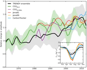
Figure 4. Trends for seasonal amplitude of TRENDY simulated multimodel ensemble mean land–atmosphere carbon flux FTA
(black), of the Mauna Loa Observatory (MLO) CO2 mixing
ra-tio (CO2MLO, green) and global CO2mixing ratio (CO2GLOBAL, purple), and of FTA from atmospheric inversions of Jena81 (red),
Jena99 (orange) and CarbonTracker (blue). The trends are relative to the 1961–1970 mean for the TRENDY ensemble and Mauna Loa CO2, and the other time series are offset to have the same mean
as the TRENDY ensemble for the last 10 years (2003–2012). A 9-year Gaussian smoothing (Harris, 1978) removes interannual vari-ability for all time series, and its 1σ standard deviation is shown for CO2MLO(green shading). Note that the gray shading here
in-stead indicates 1σ models’ spread, which is generally larger than the standard deviation of the TRENDY ensemble’s decadal variabil-ity. Inset: average seasonal cycles of models’ ensemble mean FTA
(Pg C yr−1)for the two periods: 1961–1970 (dashed line; lighter gray shading indicates 1σ model spread) and 2001–2010 (solid; darker gray shading indicates 1σ model spread), revealing enhanced CO2uptake during spring/summer growing season. Mean seasonal
cycles global FTAfrom the atmospheric inversions for 2001–2010 are also shown (same color as the main figure) for comparison.
3.2 Temporal evolution of FTAseasonal amplitude
The seasonal amplitude of global total FTA from the
TRENDY model ensemble for 1961–2012 shows a long-term rise of 19 ± 8 %, with large decadal variability (Fig. 4). Simi-larly, the seasonal amplitude of CO2at Mauna Loa increases
by 15 ± 3 % (0.85 ± 0.18 ppm) for the same period. This amplitude increase appears mostly as an earlier and deeper drawdown during the spring and summer growing season, mostly in June and July (Table 3, Fig. 4 inset). Changes in trend of yearly minima (indicating peak carbon uptake) and yearly maxima (dominated by respiration) contribute 91 ± 10 and 9 ± 10 % to the FTA amplitude increase, respectively.
Gurney and Eckels (2011) suggest trend in respiration crease is more important, but they averaged all months in-stead of using maxima and minima in their amplitude defini-tion. The multimodel ensemble mean tracks some
character-yr use
Figure 5. Attribution of the seasonal amplitude trend of global net land carbon flux for the period 1961–2012 to three key factors of CO2, climate and land use/cover. The red dots represent models’
global amplitude increase of FTAfrom the S3 experiment, and error
bars indicate 1σ standard deviation. The increasing seasonal ampli-tude of FTAis decomposed into the influence of time-varying atmo-spheric CO2(blue), climate (light green) and land use/cover change
(gold).
istics of the decadal variability reflected by the Mauna Loa record: stable in the 1960s, rise in the 1970–1980s, rapid rise in the early 2000s and decrease in the most recent 10 years. Strictly speaking, Mauna Loa CO2data are not directly
com-parable with simulated global FTAbecause this single station
is also influenced by atmospheric circulation as well as fos-sil fuel emissions and ocean–atmosphere fluxes. Neverthe-less, the comparison of the long-term amplitude trend is still valuable because the Mauna Loa Observatory data consti-tute the only long-term record, and it is generally considered representative of global mean CO2(Heimann, 1986;
Kamin-ski et al., 1996). The global total CO2 index (CO2GLOBAL)
and FTAfrom three atmospheric inversions are also included
in the comparison. All data (Jena81, CO2MLO, CO2GLOBAL)
show a decrease in seasonal amplitude in the late 1990s, pos-sibly related to drought in the Northern Hemisphere midlat-itude regions (Buermann et al., 2007; Zeng et al., 2005a), and about half of the models (LPJ, OCN, ORCHIDEE, VE-GAS) also exhibit similar change (Fig. 7). Details on models’ FTAglobal and regional changes in 2001–2010 compared to
1961–1970 are listed in Table 4.
3.2.1 Attribution of global and regional FTAseasonal
amplitude
Models agree on increase of global FTAseasonal amplitude
during 1961–2012, but they disagree even in sign in the con-tribution of the different factors (Fig. 5). By computing the ratios between amplitude trends from rising CO2, climate
change and land use/cover change with the total trend for each model, we find that the effect of varying CO2,
cli-mate and land use/cover contribute 83 ± 56, −3 ± 74 and 20 ± 30 % to the simulated global FTA amplitude increase.
All models simulate increasing amplitude for total FTA in
the boreal (50–90◦N) and northern temperate (23.5–50◦N) regions, and most models also indicate amplitude increase in the northern (0–23.5◦N) and southern tropics (0–23.5◦S) (Fig. 6). There is less agreement on the sign of amplitude change among the models in the southern extratropics (23.5–
Table 4. The seasonal amplitude (maximum minus minimum, in Pg C yr−1)of mean net carbon flux for 2001–2010 relative to the 1961–1970 period, according to the nine TRENDY models (values are listed as percentage change in brackets, for both regions and the entire globe). The four large latitudinal regions are the same as in Fig. 3: boreal (50–90◦N), temperate (23.5–50◦N), northern tropics (0–23.5◦N), southern tropics (0–23.5◦S) and southern extratropics (23.5–90◦S). Values from the two inversions, Jena99 and CarbonTracker, are also listed for comparison.
Name Global Boreal Northern Northern Southern Southern temperate tropics tropics extratropics CLM4.5BGC 44.3 (15 %) 31.9 (17 %) 19.2 (15 %) 7.2 (22 %) 6.5 (−2 %) 4.9 (4 %) ISAM 19.1 (9 %) 12.1 (11 %) 7.4 (13 %) 6.0 (1 %) 6.9 (−8 %) 0.4 (4 %) JULES 19.0 (26 %) 12.2 (24 %) 14.3 (9 %) 11.6 (0 %) 11.3 (11 %) 2.2 (−24 %) LPJ 23.4 (26 %) 23.0 (18 %) 14.7 (11 %) 10.5 (9 %) 11.8 (16 %) 2.0 (−12 %) LPX-Bern 37.9 (15 %) 26.9 (10 %) 19.3 (6 %) 8.3 (9 %) 4.6 (−6 %) 4.2 (15 %) OCN 21.6 (34 %) 12.3 (33 %) 11.1 (23 %) 9.7 (17 %) 8.3 (3 %) 2.0 (14 %) ORCHIDEE 39.9 (12 %) 23.4 (14 %) 19.1 (5 %) 22.7 (9 %) 18.7 (2 %) 1.4 (37 %) VEGAS 46.7 (15 %) 22.3 (17 %) 24.7 (10 %) 4.0 (11 %) 3.4 (12 %) 2.1 (6 %) VISIT 28.9 (14 %) 22.9 (12 %) 15.6 (8 %) 3.4 (9 %) 3.2 (1 %) 3.1 (18 %) Ensemble 26.1 (17 %) 18.0 (19 %) 12.4 (15 %) 8.0 (8 %) 4.9 (−3 %) 2.1 (13 %) Jena99 46.8 23.3 21 8.2 8.5 1.5 CarbonTracker 39.9 26.5 16.3 5.3 5.8 2.4
90◦S). Individual models’ global and regional trends of FTA
amplitude attributable to the three factors (CO2, climate and
land use/cover) are listed in Table S1. For most models, lati-tudinal contribution to global FTAamplitude (computed with
Fki
A)shows that the pronounced midlatitude to high-latitude
maxima in the NH dominate the simulated amplitude in-crease over 1961–2012 (Fig. 8, red dashed line for S3 re-sults). All models also indicate a negative contribution from at least part of the northern temperate region.
The four models (CLM4.5BGC, VEGAS, LPX-Bern and ORCHIDEE) that simulate a more realistic mean global FTA
seasonal cycle (Fig. 1) are also relatively close in global FTA seasonal amplitude, clustering around an increase of
14 ± 3 % during 1961–2012. Furthermore, they all suggest that land use/cover change contributes positively to global FTA seasonal amplitude increase. On the other hand, four
of the remaining five models (OCN, LPJ, JULES, VISIT) show a much larger rate of increase (26 ± 3 %), but given that these four models underestimate the mean amplitude by about 50 %, the absolute increase in global FTAseasonal
am-plitude is actually similar (about 5 Pg C yr−1)between the two groups of models. ISAM is an exception; it both under-estimates the mean global FTA seasonal amplitude and has
the lowest rate of amplitude increase.
3.2.2 The rising CO2factor
Seven of the nine models suggest that the CO2fertilization
effect is most responsible for the increase in the amplitude of global FTA, while VEGAS attributes it to be approximately
equal among the three factors (Fig. 5). The CO2fertilization
effect alone seems to cause most of the amplitude increase in a majority of models, with notable contribution from climate
change and land use/cover change in CLM4.5BGC and VE-GAS (Fig. 7). The effect of rising CO2appears to be slightly
negative for JULES, possibly reflecting an offsetting of the strong seasonal soil respiration response found in this model. For each model, rising CO2in the boreal, northern temperate
and the southern extratropics leads to a similar trend (Fig. 6). The magnitude of this trend may indicate each model’s dif-fering strength for CO2fertilization. This is possibly due to
similar phases of FTAseasonal cycle within the three regions
that are mainly driven by climatological temperature con-trast. The positive amplitude trend in the carbon flux of the northern and southern tropics from CO2fertilization is
simi-lar, and they likely would cancel out each other because their seasonal cycles are largely out of phase. Latitudinal contri-bution analyses reveal that the trend in the northern midlati-tudes to high-latimidlati-tudes is the main contributor to global FTA
amplitude increase when considering CO2fertilization effect
alone (Fig. 8, blue line).
3.2.3 The climate change factor
The effect of climate change on FTA amplitude is mixed:
five models (OCN, LPJ, LPX-Bern, ORCHIDEE and ISAM) suggest climate change acts to decrease the FTA amplitude,
and four models (JULES, VISIT, CLM4.5BGC and VE-GAS) suggest it is an increasing effect (Fig. 5). The high-latitude greening effect is evident in six out of nine mod-els (Fig. 6), contributing, on average, 29 % of boreal ampli-tude increase. The latitudinal contribution analyses (Fig. 8) also suggest that warming-induced high-latitude “greening” effect is present in all models, but this positive contribu-tion only exhibits a wide range of influence in about half of the models (CLM4.5BGC, JULES, VEGAS and VISIT).
yr–1 yr–1 yr–1 yr–1 yr–1 use ropics
Figure 6. Attribution of the seasonal amplitude trend of regional (boreal (50–90◦N), northern temperate (23.5–50◦N), northern tropics (0–23.5◦N), southern tropics (0–23.5◦S) and southern ex-tratropics (23.5–90◦S)) net land carbon flux for the period 1961– 2012 to three key factors CO2, climate and land use/cover. The red
dots represent models’ global amplitude increase of FTAfrom the S3 experiment. The increasing seasonal amplitude of FTAis
decom-posed into the influence of time-varying atmospheric CO2(blue),
climate (light green) and land use/cover change (gold).
The latitudinal patterns also reveal that, once climate change is considered, the contribution from the northern temper-ate region around 40◦N shifts to negative in all models. In the northern temperate (23.5–50◦N) region, climate change
alone would decrease the FTA amplitude – this is
con-sistent among the four models with realistic mean global and northern temperate (Fig. 2) FTA seasonal cycle
simula-tion, but is not the case for JULES and LPJ (Fig. 6). Such decrease is possibly related to midlatitude drought (Buer-mann et al., 2007), which is consistent with findings by Schneising et al. (2014), who observed a negative relation-ship between temperature and seasonal amplitude of xCO2
from both satellite measurements and CarbonTracker dur-ing 2003–2011 for the Northern temperate zone. The neg-ative contribution from the temperate zone counteracts the positive boreal contribution, suggesting that the net impact from climate change on FTAamplitude may not be as
signif-icant as previously suggested. With changing climate intro-duced, some models exhibit similar characteristics of decadal variability in global FTAamplitude (Fig. 7). OCN and
OR-CHIDEE appear to be especially sensitive to the climate
vari-c
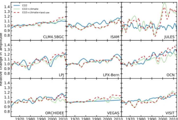
c c land use
Figure 7. Trends for seasonal amplitude of global total net carbon fluxes from S1 (CO2), S2 (CO2+climate) and S3
(CO2+climate+land use) for each individual TRENDY model. All amplitude time series are relative to their own 1961–1970 mean am-plitude.
ations after the 1990s, resulting in a decrease in FTA
am-plitude. It is also apparent from the time series figure that the strong increasing trend of FTA amplitude from climate
change in JULES is mostly due to the sharp rise from early 1990s to early 2000s, suggesting some possible model arti-facts (Fig. 7). The effect of climate change is more mixed in both tropics and the southern extratropics.
3.2.4 The land use/cover change factor
Six of the nine models show that land use/cover change leads to increasing global FTA amplitude (Fig. 5). Land use/cover
change appears to amplify FTAseasonal cycle in boreal and
northern temperate regions for most models. For some mod-els (VEGAS, CLM4.5BGC and OCN), this effect is espe-cially pronounced in the northern temperate region where most of the global crop production takes place (Fig. 6). Note that the effect of land use/cover change includes two parts: one is the change of land use practice without changing the land cover type; the other is the change of land cover, in-cluding crop abandonment etc. VEGAS simulates the time-varying management intensity and the crop harvest index, which is an example of significant contribution from land use change (Zeng et al., 2014). For many other models, crops are treated as generic managed grasslands (i.e., CLM4.5BGC, LPJ), and land cover change is possibly the more important factor. During 1961–2012, large cropland areas were aban-doned in the eastern United States and central Europe, and forest regrowth often followed. New cropland expanded in the tropics and South America, midwestern United States, eastern and central North Asia and the Middle East. How such changes affect the global FTAamplitude is determined
by the productivity and seasonal phase of the old and new vegetation covers. For CLM4.5BGC, JULES, LPJ and
OR-CHIDEE, enhanced vegetation activity from growing forest in these regions contributes positively to global FTA
am-plitude increase (Fig. 9). In contrast, for LPX-Bern, VISIT and VEGAS in the eastern United States, a loss of cropland leads to a decrease in the amplitude. Additional cropland in the midwestern United States and eastern and central North Asia contributes negatively to the FTA amplitude trend for
JULES, LPJ and ORCHIDEE. These regions, however, are major zones contributing to the amplification of global FTA
for LPX-Bern, OCN, VEGAS and VISIT. One mechanism mentioned previously is agricultural intensification in VE-GAS: in fact, CO2flux measurements over corn fields in the
US Midwest show much larger seasonal amplitude than over nearby natural vegetation (Miles et al., 2012). Similarly, al-though croplands are treated as generic grassland, they still receive time-varying and spatially explicit fertilizer input in OCN (Zaehle et al., 2011). Another plausible mechanism is irrigation, which can alleviate adverse climate impact from droughts, and crops may have a stronger seasonal cycle than the natural vegetation they replace in these regions. The over-all effect of land use/cover change for each model, there-fore, is often the aggregated result over many regions that can only be revealed by spatially explicit patterns. When exam-ining the latitudinal contribution only (Fig. 8), CLM4.5BGC, LPX-Bern, OCN and VEGAS are quite similar, even though the spatial patterns reveal that CLM4.5BGC is very different from the other three models (Fig. 9). For JULES, LPJ and ORCHIDEE a significant part of land use/cover change con-tribution comes from the tropical zone (Fig. 8). While most models indicate that land use/cover change in the southern tropics (Amazon is probably the most notable region) de-creases global FTA amplitude during 1961–2012, LPJ
sug-gests that it would cause a large increase in the amplitude instead, possibly related to its different behavior in simulat-ing the mean seasonal cycle of carbon flux for that region (Fig. 2d).
4 Discussion and conclusion
Our results show a robust increase of global and regional (es-pecially over the boreal and northern temperate regions) FTA
amplitude simulated by all TRENDY models. During 1961–
2012, TRENDY models’ ensemble mean global FTArelative
amplitude increases (19 ± 8 %). Similarly, the CO2
ampli-tude also increases (15 ± 3 %) at Mauna Loa for 1961–2012. This amplitude increase mostly reflects the earlier and deeper
drawdown of CO2 in the NH growing season. The models
in general, especially the multimodel median, simulate lat-itudinal patterns of FTA mean amplitude that are similar to
the atmospheric inversions results. Their latitudinal patterns capture the temperature-driven seasonality from the NH mid-latitude to high-mid-latitude region and the two monsoon-driven subtropical maxima, although the magnitude or extent vary. Despite the general agreements between the models’
ensem-Figure 8. Latitudinal contribution of trends for seasonal amplitude of global land–atmosphere carbon flux from TRENDY models in the three sensitivity experiments. Fluxes are summed over each 2.5◦ latitude band (Pg C yr−1 per 2.5◦ latitude) before computing the Fki
A(refer to the Methodology section for definition). For each 2.5
◦
latitude band, the trend is calculated for the period 1961–2012.
Figure 9. Contribution from land use/cover change on trends in the seasonal amplitude of global land–atmosphere carbon flux. For each spatial grid, the trend is computed as trends of the Fki
A (refer to
Methodology section for definition) in the S3 experiment (changing CO2, climate and land use/cover) subtracted by trends in S2
(chang-ing CO2and climate).
ble amplitude increases and the limited observation-based es-timates, considerable model spread is noticeable. Five of the nine models considerably underestimate the global mean FTA
seasonal cycle compared to atmospheric inversions, and peak carbon uptake takes place 1 or 2 months too early in seven of the nine models. The seasonal amplitude of model
ensem-ble global mean FTAis 40 % smaller than the amplitude of
the atmosphere inversions. In contrast to the divergence in simulated seasonal carbon cycle, atmospheric inversions in Northern temperate and boreal regions are well constrained: 11 different inversions agree on July FTA minimum in the
Northern Hemisphere (25–90◦N), with no more than 20 %
difference in amplitude (Peylin et al., 2013).
The simulated amplitude increase is found to be mostly
due to a larger FTA minimum associated with a stronger
ecosystem growth. Over the historical period, global mean carbon sink also increases over time, suggesting a possible relationship between seasonal amplitude and the mean sink (Ito et al., 2016; Randerson et al., 1997; Zhao and Zeng, 2014). The increasing trend of CO2 amplitude, dominated
by increasing trend of FTAamplitude, has been interpreted as
evidence for steadily increasing net land carbon sink (Keel-ing et al., 1995; Prentice et al., 2000). However, the increas-ing amplitude could also arise from (climatically induced) increased phase separation of photosynthesis and respiration, e.g., due to warming-induced earlier greening (Myneni et al., 1997). For the nine models, we found a moderate relationship between enhanced mean land carbon sink and the seasonal amplitude increase similar to reported results by in Zhao and Zeng (2014), with an R-squared value of 0.61 (Fig. 10). There might be some possibility in constraining change in
land carbon sink with changes in observed CO2 seasonal
amplitude; however, extra caution should be given when in-terpreting this global-scale cross-model correlation, as there could be important regional differences that cancel out in ag-gregated global values. A factorial analysis of the long-term carbon uptake could help to determine which factor con-tributes to what extent to this correlation. Further research is also needed to explore the mechanisms behind such a re-lationship at continental scale, where more data from well-calibrated CO2monitoring sites and data on air–sea fluxes
and atmospheric vertical transport could better constrain car-bon balance (Prentice et al., 2001). Changes in residual land carbon sink estimates are also shown (Fig. 10), with the caveat that it is not directly comparable with simulated net carbon sink increase if there is a trend in simulated carbon flux changes associated with land cover conversion (defor-estation, crop abandonment, etc.). Additionally, the decadal changes in residual and net land carbon sink are far from linear; instead, a sudden increase in mean land uptake oc-curred in 1988 (Beaulieu et al., 2012; Rafique et al., 2016; Sarmiento et al., 2010). With the aid of atmospheric trans-port, CO2amplitude trends at remote sites have
benchmark-ing potential to constrain the models, especially with more observations and improved understanding of vegetation dy-namics at regional level in the near future.
Models with a strong mean carbon sink (for example JULES and OCN) can have relatively weak seasonal ampli-tude, and the LPX-Bern model shows no carbon sink despite having a strong FTAseasonality. Based on data from Table 8
of the Global Carbon Budget report (Le Quéré et al., 2014),
r
Figure 10. Relationship between the increase in net biosphere pro-duction (NBP, equal to −FTA)and increase in NBP seasonal
am-plitude (as in Fig. 4’s red dots), for the 1961–2012 period for nine TRENDY models. Error bars indicate the standard errors of the trend estimates. Increase in residual land sink is estimated by tak-ing the difference between two residual land sinks, over 2004–2013 and 1960–1969 (an interval of 44 years), as reported in Le Quéré et al. (2015). This difference is then scaled by 52/44 (to make it comparable with models’ NBP change for this figure), which is dis-played by a black vertical line and shading (error added in quadra-ture, assuming Gaussian error for the two decadal residual land sinks, then also scaled). The cross-model correlation (R2=0.61, p< 0.05) suggests that a model with a larger net carbon sink in-crease is likely to simulate a higher inin-crease in NBP seasonal am-plitude.
the net land carbon sink for 2000–2009 is estimated to be 1.5 ± 0.7 Pg C yr−1(assuming Gaussian errors). Four models (JULES, OCN, VEGAS and VISIT) examined in this study are within the uncertainty range of this budget-based analy-sis. In spite of their similar mean land carbon sink, the shape of their FTAseasonal cycle differs. While VEGAS also shows
a similar seasonal carbon cycle compared to inversions, the other three models exhibit an unrealistically long carbon up-take period with half the amplitude as the inversions. July and August are the only 2 months with net carbon release for JULES, whereas OCN and VISIT both have a long ma-jor carbon uptake period from May to September. Given that the mean global and regional FTA seasonal cycles are
rela-tively well constrained in the northern extratropics, they can serve as a benchmark for terrestrial models (Heimann et al., 1998; Prentice et al., 2001). Insights gained from analyzing modeled seasonal amplitude of carbon flux may help to un-derstand the considerable model spread found in the mean global carbon sink for the historical period (Le Quéré et al., 2015), which is possibly due to varied model sensitivity to different mechanisms (Arora et al., 2013). Examining details of different representations of important processes in models
could also help to better assess the different future projec-tions on both the magnitude and direction of global carbon flux (Friedlingstein et al., 2006, 2013).
Unlike many previous studies that focused on comparing the season cycle at individual CO2monitoring stations (Peng
et al., 2015; Randerson et al., 1997), we studied the global and large latitudinal bands. Such quantities often demon-strate well-constrained seasonality that is relatively robust against uncertainty from atmospheric transport, fossil fuel emission and biomass burning etc. We found greater uncer-tainty for the tropics and southern extratropics regions where atmospheric CO2 observations are relatively sparse.
Tropi-cal ecosystems are also heavily affected by biomass burning; however, some models used in this study do not include fire dynamics. For models that simulate fire ignition/suppression, they are also varied by structure and complexity of fire-related processes, and many of them are prognostic (Poulter et al., 2015). It is not clear how fire would affect the FTA
sea-sonal cycle at global scale, and recent sensitivity study shows only minor differences among fire and “no fire” scenarios in CO2 seasonal cycle at several observation stations (Poulter
et al., 2015). These uncertainties, however, are unlikely to affect our main conclusions because of the limited contri-bution of tropics to global FTA amplitude increase. Another
possibly important factor is the impact from increased nitro-gen deposition, which may have been included in the “CO2
fertilization” effect for some models with full nitrogen cycle (Table 1); however, this can only be explored in future stud-ies, as the TRENDY experiment design does not separate out the nitrogen contribution.
Our factorial analyses highlight fundamentally differential control from rising CO2, climate change and land use/cover
change among the models, with seven out of nine mod-els indicating major contribution (83 ± 56 %) to global FTA
amplitude increase from the CO2 fertilization effect. The
strength of CO2 fertilization varies among models, but for
each model, its magnitude in the boreal, northern temper-ate and southern extratropics regions is similar. Models are split regarding the role of climate change, as compared with the models’ ensemble mean (−3 ± 74 %). Regional analy-ses show that climate change amplifies the boreal FTA
sea-sonal cycle but weakens the seasea-sonal cycle for other regions according to most models. By examining latitudinal trends from Fki
A, we found all models indicate a negative climate
contribution over the midlatitudes, where droughts might have reduced ecosystem productivity. This negative effect offsets the high-latitude greening, which in some models re-sults in a net negative climate change impact on global FTA
amplitude. Such a mechanism casts doubt on whether cli-mate change is the main driver of the global FTAamplitude
increase. Land use/cover change, according to majority of the models, appears to amplify the global FTAseasonal cycle
(20 ± 30 %); however, the mechanisms seem to differ among models. Conversion to/from cropland could either increase or decrease the seasonal amplitude, depending on how models
simulate the seasonal cycle of cropland compared to the nat-ural vegetation it replaces/precedes. For the same pattern of increasing amplitude, the underlying causes could include ir-rigation mitigating negative climate effect, agricultural man-agement practices and other mechanisms.
Overall, this study is largely helpful to enhance our un-derstanding of the role of CO2, climate change and land
use/cover change in regulating the seasonal amplitude of car-bon fluxes. In particular, models’ disagreement in spatial pat-tern of carbon flux amplitude helps to identify optimal loca-tions for additional CO2observations in the north. However,
this work can be further improved through utilizing the CO2
seasonal cycle and its amplitude at different locations as in-dicators to diagnose model behaviors. To achieve this, it is necessary to apply atmosphere transport on the simulated net carbon flux, along with ocean and fossil fuel fluxes, which would allow direct comparison with observed CO2amplitude
change. In doing so, it is possible that models may overesti-mate CO2 amplitude increase at most CO2observation
sta-tions if the simulated CO2fertilization effect is too strong.
5 Data availability
Results of TRENDY models analyzed in this study will be available on request by the end of 2016 (please contact S. Sitch at s.a.sitch@exeter.ac.uk for further updates and de-tails).
Appendix A: Environmental drivers for TRENDY
For observed rising atmospheric CO2 concentration, the
models use a single global annual (1860–2012) time se-ries from ice cores (before 1958: Joos and Spahni, 2008) and the National Oceanic and Atmospheric Administration (NOAA)’s Earth System Research Laboratory (after 1958:
monthly average from Mauna Loa and South Pole CO2;
South Pole data are constructed from the 1976–2014 aver-age if not available). For climate forcing, the models em-ploy 1901–2012 global climate data from the Climate Re-search Unit (CRU, version TS3.21, http://www.cru.uea.ac. uk; or CRU-National Centers for Environmental Prediction (NCEP) dataset, version 4, from N. Viovy (2011), unpub-lished data) at monthly (or interpolated to finer temporal resolution for individual models) temporal resolution and 0.5◦×0.5◦spatial resolution. For land use/cover change
his-tory data, the models adopt either gridded yearly cropland and pasture fractional cover from the History Database of the Global Environment (HYDE) version 3.1 (http://themasites. pbl.nl/tridion/en/themasites/hyde/, (Klein Goldewijk et al., 2011), or the dataset including land use history transitions from L. Chini based on the HYDE data.
Appendix B: Atmospheric inversions
The Jena inversion is from the Max Planck Institute of Bio-geochemistry, v3.7, at 5◦×5◦spatial resolution (http://www. bgc-jena.mpg.de/christian.roedenbeck/download-CO2/, Rö-denbeck et al., 2003), including two datasets abbreviated as Jena81 for the period of 1981–2010 using CO2data from 15
stations, and Jena99 using 61 stations for 1999–2010. An-other inversion-based dataset used is the CarbonTracker, ver-sion CT2013B, from NOAA/ESRL at 1◦×1◦spatial resolu-tion (http://www.esrl.noaa.gov/gmd/ccgg/carbontracker/, Pe-ters et al., 2007) for the period of 2000–2010, which inte-grates flask samples from 81 stations, 13 continuous mea-surement stations and 9 flux towers, and the surface fluxes from land and ocean carbon models as prior fluxes. These two inversion-based datasets are vastly different in their ap-proach in inversion algorithm, choice of atmospheric data, transport model and prior information (Peylin et al., 2013). For example, to minimize the spurious variability introduced by changes in availability of observations, the Jena inver-sion provides multiple verinver-sions with different record length, each only using records covering its full period (for example, Jena99 includes more stations than Jena81, but with a shorter period). The CarbonTracker, however, opts for assimilating all quality-controlled data (with outliers removed), favoring a higher spatial resolution in estimated carbon fluxes. There-fore, we chose these two inversions to capture the uncertainty in atmospheric inversions to some extent.
The Supplement related to this article is available online at doi:10.5194/bg-13-5121-2016-supplement.
Author contributions. Fang Zhao and Ning Zeng designed the study and Fang Zhao carried it out. Shijie Sitch and Pierre Friedling-stein designed and coordinated TRENDY experiments. TRENDY modelers conducted the simulations. Fang Zhao wrote the paper with input from all authors.
Acknowledgements. This study was funded by NOAA, NASA and NSF. This study was partly supported by a Laboratory Directed Research and Development project by Pacific Northwest National Laboratory that is being managed by Battelle Memo-rial Institute for the US Department of Energy. We thank the TRENDY coordinators and participating modeling teams, NOAA ESRL and Jena/CarbonTracker inversion teams. TRENDY model results used in this study may be obtained from S. Sitch (email: s.a.sitch@exeter.ac.uk).
Edited by: A. V. Eliseev
Reviewed by: two anonymous referees
References
Alexandrov, G. A.: Explaining the seasonal cycle of the globally averaged CO2with a carbon-cycle model, Earth Syst. Dynam.,
5, 345–354, doi:10.5194/esd-5-345-2014, 2014.
Arora, V. K., Boer, G. J., Friedlingstein, P., Eby, M., Jones, C. D., Christian, J. R., Bonan, G., Bopp, L., Brovkin, V., Cad-ule, P., Hajima, T., Ilyina, T., Lindsay, K., Tjiputra, J. F., and Wu, T.: Carbon–Concentration and Carbon–Climate Feedbacks in CMIP5 Earth System Models, J. Clim., 26, 5289–5314, doi:10.1175/JCLI-D-12-00494.1, 2013.
Bacastow, R. B., Keeling, C. D., and Whorf, T. P.: Seasonal am-plitude increase in atmospheric CO2 concetration at Mauna
Loa, Hawaii, 1959–1982, J. Geophys. Res., 90, 10529–10540, doi:10.1029/JD090iD06p10529, 1985.
Beaulieu, C., Sarmiento, J. L., Mikaloff Fletcher, S. E., Chen, J., and Medvigy, D.: Identification and characterization of abrupt changes in the land uptake of carbon, Global Biogeochem. Cy., 26, 1–14, doi:10.1029/2010GB004024, 2012.
Buermann, W., Lintner, B. R., Koven, C. D., Angert, A., Pinzon, J. E., Tucker, C. J., and Fung, I. Y.: The changing carbon cycle at Mauna Loa Observatory, P. Natl. Acad. Sci. USA, 104, 4249– 4254, 2007.
Clark, D. B., Mercado, L. M., Sitch, S., Jones, C. D., Gedney, N., Best, M. J., Pryor, M., Rooney, G. G., Essery, R. L. H., Blyth, E., Boucher, O., Harding, R. J., Huntingford, C., and Cox, P. M.: The Joint UK Land Environment Simulator (JULES), model descrip-tion – Part 2: Carbon fluxes and vegetadescrip-tion dynamics, Geosci. Model Dev., 4, 701–722, doi:10.5194/gmd-4-701-2011, 2011. Collins, W. J., Bellouin, N., Doutriaux-Boucher, M., Gedney, N.,
Halloran, P., Hinton, T., Hughes, J., Jones, C. D., Joshi, M., Lid-dicoat, S., Martin, G., O’Connor, F., Rae, J., Senior, C., Sitch,
S., Totterdell, I., Wiltshire, A., and Woodward, S.: Develop-ment and evaluation of an Earth-System model – HadGEM2, Geosci. Model Dev., 4, 1051–1075, doi:10.5194/gmd-4-1051-2011, 2011.
Dalmonech, D. and Zaehle, S.: Towards a more objective evalua-tion of modelled land-carbon trends using atmospheric CO2and
satellite-based vegetation activity observations, Biogeosciences, 10, 4189–4210, doi:10.5194/bg-10-4189-2013, 2013.
Dalmonech, D., Zaehle, S., Schürmann, G. J., Brovkin, V., Reick, C., and Schnur, R.: Separation of the Effects of Land and Climate Model Errors on Simulated Contemporary Land Carbon Cycle Trends in the MPI Earth System Model version 1*, J. Clim., 28, 272–291, doi:10.1175/JCLI-D-13-00593.1, 2015.
Forkel, M., Carvalhais, N., Schaphoff, S., v. Bloh, W., Migliavacca, M., Thurner, M., and Thonicke, K.: Identifying environmental controls on vegetation greenness phenology through model-data integration, Biogeosciences, 11, 7025–7050, doi:10.5194/bg-11-7025-2014, 2014.
Forkel, M., Carvalhais, N., Rödenbeck, C., Keeling, R., Heimann, M., Thonicke, K., Zaehle, S., and Reichstein, M.: En-hanced seasonal CO2 exchange caused by amplified plant
productivity in northern ecosystems, Science, 351, 696–699, doi:10.1126/science.aac4971, 2016.
Friedlingstein, P., Cox, P., Betts, R., Bopp, L., Von Bloh, W., Brovkin, V., Cadule, P., Doney, S., Eby, M., Fung, I., Bala, G., John, J., Jones, C., Joos, F., Kato, T., Kawamiya, M., Knorr, W., Lindsay, K., Matthews, H. D., Raddatz, T., Rayner, P., Reick, C., Roeckner, E., Schnitzler, K. G., Schnur, R., Strassmann, K., Weaver, A. J., Yoshikawa, C., and Zeng, N.: Climate-carbon cy-cle feedback analysis: Results from the (CMIP)-M-4 model in-tercomparison, J. Clim., 19, 3337–3353, doi:10.1175/jcli3800.1, 2006.
Friedlingstein, P., Meinshausen, M., Arora, V. K., Jones, C. D., Anav, A., Liddicoat, S. K., and Knutti, R.: Uncertainties in CMIP5 climate projections due to carbon cycle feedbacks, J. Clim., 27, 511–526, doi:10.1175/JCLI-D-12-00579.1, 2013. Graven, H. D., Keeling, R. F., Piper, S. C., Patra, P. K., Stephens,
B. B., Wofsy, S. C., Welp, L. R., Sweeney, C., Tans, P. P., Kelley, J. J., Daube, B. C., Kort, E. A., Santoni, G. W., and Bent, J. D.: Enhanced Seasonal Exchange of CO2 by
Northern Ecosystems Since 1960, Science, 341, 1085–1089, doi:10.1126/science.1239207, 2013.
Gray, J. M., Frolking, S., Kort, E. A., Ray, D. K., Kucharik, C. J., Ramankutty, N., and Friedl, M. A.: Direct human influence on atmospheric CO2seasonality from increased cropland
produc-tivity, Nature, 515, 398–401, doi:10.1038/nature13957, 2014. Gurney, K. R. and Eckels, W. J.: Regional trends in terrestrial
car-bon exchange and their seasonal signatures, Tellus B, 63, 328– 339, doi:10.1111/j.1600-0889.2011.00534.x, 2011.
Hall, C. A. S., Ekdahl, C. A., and Wartenberg, D. E.: A fifteen-year record of biotic metabolism in the Northern Hemisphere, Nature, 255, 136–138, doi:10.1038/255136a0, 1975.
Harris, F. J.: On the use of windows for harmonic analy-sis with the discrete Fourier transform, P. IEEE, 66, 51–83, doi:10.1109/PROC.1978.10837, 1978.
Heimann, M.: The Changing Carbon Cycle, a Global Analysis, edited by: Trabalka, J. R. and Reichle, D. E., Springer, New York, 1986.
Heimann, M., Esser, G., Haxeltine, A., Kaduk, J., Kicklighter, D. W., Knorr, W., Kohlmaier, G. H., Mcguire, A. D., Melillo, J., Moore, B., Ottofi, R. D., Prentice, I. C., Sauf, W., Schloss, A., Sitch, S., Wittenberg, U., and Wtirth, G.: Evaluation of terrestrial carbon cycle models through simulations of the seasonal cycle of atmospheric First results of a model intercomparison study, Global Biogeochem. Cy., 12, 1–24, 1998.
Huntzinger, D. N., Schwalm, C., Michalak, A. M., Schaefer, K., King, A. W., Wei, Y., Jacobson, A., Liu, S., Cook, R. B., Post, W. M., Berthier, G., Hayes, D., Huang, M., Ito, A., Lei, H., Lu, C., Mao, J., Peng, C. H., Peng, S., Poulter, B., Riccuito, D., Shi, X., Tian, H., Wang, W., Zeng, N., Zhao, F., and Zhu, Q.: The North American Carbon Program Multi-Scale Synthesis and Terrestrial Model Intercomparison Project – Part 1: Overview and experimental design, Geosci. Model Dev., 6, 2121–2133, doi:10.5194/gmd-6-2121-2013, 2013.
Ito, A., Inatomi, M., Huntzinger, D., Schwalm, C., Michalak, A., Cook, R., King, A., Mao, J., Wei, Y., Post, W. Mac, Wang, W., Arain, M. A., Huang, S., Hayes, D., Ricciuto, D., Shi, X., Huang, M., Lei, H., Tian, H., Lu, C., Yang, J., Tao, B., Jain, A., Poul-ter, B., Peng, S., Ciais, P., Fisher, J., Parazoo, N., Schaefer, K., Peng, C., Zeng, N., and Zhao, F.: Decadal trends in the seasonal-cycle amplitude of terrestrial CO2exchange resulting from the
ensemble of terrestrial biosphere models, Tellus B, 68, 28968, doi:10.3402/tellusb.v68.28968, 2016.
Jain, A. K., Meiyappan, P., Song, Y., and House, J. I.: CO2
emis-sions from land-use change affected more by nitrogen cycle, than by the choice of land-cover data, Glob. Change Biol., 19, 2893– 906, doi:10.1111/gcb.12207, 2013.
Joos, F. and Spahni, R.: Rates of change in natural and anthropogenic radiative forcing over the past 20,000 years, P. Natl. Acad. Sci. USA, 105, 1425–1430, doi:10.1073/pnas.0707386105, 2008.
Kaminski, T., Giering, R., and Heimann, M.: Sensitivity of the sea-sonal cycle of CO2 at remote monitoring stations with respect to seasonal surface exchange fluxes determined with the adjoint of an atmospheric transport model, Phys. Chem. Earth, 21, 457– 462, 1996.
Kato, E., Kinoshita, T., Ito, A., Kawamiya, M., and Yama-gata, Y.: Evaluation of spatially explicit emission scenario of land-use change and biomass burning using a process-based biogeochemical model, J. Land Use Sci., 8, 104–122, doi:10.1080/1747423X.2011.628705, 2013.
Keeling, C. D., Whorf, T. P., Wahlen, M., and van der Plichtt, J.: In-terannual extremes in the rate of rise of atmospheric carbon diox-ide since 1980, Nature, 375, 666–670, doi:10.1038/375666a0, 1995.
Keeling, C. D., Chin, J. F. S., and Whorf, T. P.: Increased activity of northern vegetation inferred from atmospheric CO2
measure-ments, Nature, 382, 146–149, doi:10.1038/382146a0, 1996. Keenan, T., Gray, J., and Friedl, M.: Net carbon uptake
has increased through warming-induced changes in temper-ate forest phenology, Nature Climtemper-ate Change, 4, 598–604, doi:10.1038/NCLIMATE2253, 2014.
Klein Goldewijk, K., Beusen, A., Van Drecht, G., and De Vos, M.: The HYDE 3.1 spatially explicit database of human-induced global land-use change over the past 12,000 years, Global Ecol. Biogeogr., 20, 73–86, doi:10.1111/j.1466-8238.2010.00587.x, 2011.
Krinner, G., Viovy, N., de Noblet-Ducoudré, N., Ogée, J., Polcher, J., Friedlingstein, P., Ciais, P., Sitch, S., and Prentice, I. C.: A dynamic global vegetation model for studies of the cou-pled atmosphere-biosphere system, Global Biogeochem. Cy., 19, GB1015, doi:10.1029/2003GB002199, 2005.
Le Quéré, C., Peters, G. P., Andres, R. J., Andrew, R. M., Boden, T. A., Ciais, P., Friedlingstein, P., Houghton, R. A., Marland, G., Moriarty, R., Sitch, S., Tans, P., Arneth, A., Arvanitis, A., Bakker, D. C. E., Bopp, L., Canadell, J. G., Chini, L. P., Doney, S. C., Harper, A., Harris, I., House, J. I., Jain, A. K., Jones, S. D., Kato, E., Keeling, R. F., Klein Goldewijk, K., Körtzinger, A., Koven, C., Lefèvre, N., Maignan, F., Omar, A., Ono, T., Park, G.-H., Pfeil, B., Poulter, B., Raupach, M. R., Regnier, P., Röden-beck, C., Saito, S., Schwinger, J., Segschneider, J., Stocker, B. D., Takahashi, T., Tilbrook, B., van Heuven, S., Viovy, N., Wan-ninkhof, R., Wiltshire, A., and Zaehle, S.: Global carbon budget 2013, Earth Syst. Sci. Data, 6, 235–263, doi:10.5194/essd-6-235-2014, 2014.
Le Quéré, C., Moriarty, R., Andrew, R. M., Peters, G. P., Ciais, P., Friedlingstein, P., Jones, S. D., Sitch, S., Tans, P., Arneth, A., Boden, T. A., Bopp, L., Bozec, Y., Canadell, J. G., Chini, L. P., Chevallier, F., Cosca, C. E., Harris, I., Hoppema, M., Houghton, R. A., House, J. I., Jain, A. K., Johannessen, T., Kato, E., Keel-ing, R. F., Kitidis, V., Klein Goldewijk, K., Koven, C., Landa, C. S., Landschützer, P., Lenton, A., Lima, I. D., Marland, G., Mathis, J. T., Metzl, N., Nojiri, Y., Olsen, A., Ono, T., Peng, S., Peters, W., Pfeil, B., Poulter, B., Raupach, M. R., Regnier, P., Rö-denbeck, C., Saito, S., Salisbury, J. E., Schuster, U., Schwinger, J., Séférian, R., Segschneider, J., Steinhoff, T., Stocker, B. D., Sutton, A. J., Takahashi, T., Tilbrook, B., van der Werf, G. R., Viovy, N., Wang, Y.-P., Wanninkhof, R., Wiltshire, A., and Zeng, N.: Global carbon budget 2014, Earth Syst. Sci. Data, 7, 47–85, doi:10.5194/essd-7-47-2015, 2015.
Masarie, K. A. and Tans, P. P.: Extension and integration of atmospheric carbon dioxide data into a globally con-sistent measurement record, J. Geophys. Res., 100, 11593, doi:10.1029/95JD00859, 1995.
McGuire, A. D., Sitch, S., Clein, J. S., Dargaville, R., Esser, G., Foley, J., Heimann, M., Joos, F., Kaplan, J., Kicklighter, D. W., Meier, R. A., Melillo, J. M., Moore III, B., Prentice, I. C., Ra-mankutty, N., Reichenau, T., Schloss, A., Tian, H., Williams, L. J., and Wittenberg, U.: Carbon balance of the terrestrial biosphere in the twentieth century: Analyses of CO2, climate and land use
effects with four process-based ecosystem models, Global Bio-geochem. Cy., 15, 183–206, 2001.
Miles, N. L., Richardson, S. J., Davis, K. J., Lauvaux, T., Andrews, A. E., West, T. O., Bandaru, V., and Crosson, E. R.: Large am-plitude spatial and temporal gradients in atmospheric boundary layer CO2mole fractions detected with a tower-based network
in the U.S. upper Midwest, J. Geophys. Res.-Biogeo., 117, 1–13, doi:10.1029/2011JG001781, 2012.
Myneni, R. B., Keeling, C. D., Tucker, C. J., Asrar, G., and Nemani, R. R.: Increased plant growth in the northern high latitudes from 1981 to 1991, Nature, 386, 698–702, doi:10.1038/386698a0, 1997.
Oleson, K., Lawrence, D., Bonan, G., Drewniak, B., Huang, M., Koven, C., Levis, S., Li, F., Riley, W., Subin, Z., Swenson, S., Thornton, P., Bozbiyik, A., Fisher, R., Heald, C., Kluzek, E., Lamarque, J.-F., Lawrence, P., Leung, L., Lipscomb, W.,