Carbon dynamics of global land use, land-use change, and forestry

Carbon Dynamics

Of Global Land Use, Land-Use Change, and Forestry

Erik S. Landry

S.B., Chemistry University of Chicago, 2013

Submitted to the Institute for Data, Systems, and Society in Partial Fulfillment of the Requirements for the Degree

of

Master of Science in Technology and Policy at the

MASSACHUSETTS INSTITUTE OF TECHNOLOGY June 2018

c 2018 Massachusetts Institute of Technology. All rights reserved.

Signature redacted

Signature of Author ... ...

Technology an Policy Program Institute for Data, Systems, and Society May 18, 2018

Signature

redacted

Certified by ... ...

John D. Sterman ay W. Forrester Professor of Management Thesis Supervisor

Signature redacted

Accepted by ... ... ...

Munther Dahleh

MASSACHUSETTS NSTITUTE _{Professor of Electrical Engineering and Computer Science}

Director, Institute for Data, Systems, and Society

Carbon Dynamics

Of Global Land Use, Land-Use Change, and Forestry

Erik S. Landry

Submitted to the Institute for Data, Systems, and Society on May 18, 2018 in Partial Fulfillment of the Requirements for the Degree of Master of Science in

Technology and Policy

Abstract

Forest harvest for bioenergy is growing rapidly, spurred by the European Commission's declaration that bioenergy is carbon-neutral. Bioenergy advocates argue that the carbon released upon the combustion of harvested wood should eventually be reabsorbed from the atmosphere when the harvested land regrows. Recent studies, however, find that wood bioenergy can exacerbate climate change because it is less efficient than the fossil fuels it displaces, and because regrowth takes time and is uncertain. Other land use, land-use change, and forestry (LULUCF) practices can also cause significant carbon fluxes to and from the atmosphere that vary over time as the carbon sequestered in the biomass and soils on each land type changes. Understanding these complex interactions requires an explicit dynamic model that accounts for various land uses and regions, each with carbon content and flux characteristics specific to their respective vegetation, soil distributions, and climatic domains. This work extends the widely used C-ROADS climate model, originally developed with a single biosphere, to incorporate this level of detail. Built up from a diverse set of highly resolved geospatial databases for land cover, soils, climatic domains, and other relevant characteristics, the model aggregates the data into six land use types (natural forest, harvested forest, cropland, pasture, permafrost, and developed/other land) within six major regions (the US, EU, China, India, Other Developed Nations, and Other Developing Nations). It is used to analyze the impact of harvesting forests for bioenergy. Because wood bioenergy is less efficient than the fossil fuels it displaces, the first impact is an increase in atmospheric CO2. If the land regrows as forest, this carbon debt can eventually be repaid. However, the time required to do so is long, ranging from 20 to 186 years, depending on the region supplying the wood and whether the forest is thinned or clear-cut. Converting forest to cropland after harvest increases atmospheric CO2 concentrations without payback. Results also show that

afforestation programs are most effective in reducing atmospheric CO2 when implemented in regions with

more tropical climates due to the higher carbon density of these forests. This fast, regionally specific, multi-land-use model enables policy makers and other stakeholders to quickly design and evaluate of a wide range of LULUCF and bioenergy policy scenarios and their climatic effects.

Thesis Supervisor: John D. Sterman

TABLES

TA BLE 1. L A N D U SE M A PPIN G ... ₁₀

TABLE 2. PARAMETERS OF INTEREST, SPECIFIC TO LAND USE, U, AND REGION, R... 19

TABLE Sl. MAPPING: FAO COUNTRY TO C-ROADS REGIONS ... 37

TABLE S2. FA O LAND U SE D EFINITIONS ... 43

TABLE S3. MAPPING BETWEEN IPCC LAND USE, ESA CCI LAND COVER, AND GLC2000 LAND COVER ... 45

TABLE S4. FAO FRAMEWORK FOR CLIMATIC AND ECOLOGICAL CLASSIFICATION ... 47

TABLE S5. MAPPING: TREE SPECIES INTO FAO ECOLOGICAL DOMAINS ... 47

TABLE S6. IPCC ANNUAL EMISSION FACTORS (EF) FOR CULTIVATED ORGANIC SOILS WITH FAO MAPPING...50

TABLE S7. IPCC ANNUAL EMISSION FACTORS (EF) FOR DRAINED GRASSLAND AND ORGANIC SOILS WITH FAO M A PP IN G ... 5 0 EQUATIONS EQUATION 1. CHANGE IN BIOMASS CARBON STOCK ... 9

EQUATION 2. NET PRIMARY PRODUCTION (MODIFIED RICHARDS GROWTH FUNCTION)...9

EQUATION 3. CHANGE IN SOIL CARBON STOCK ... 9

EQUATION 4. NET PRIMARY PRODUCTION OF CROPLANDS AND PASTURE ... 18

EQUATION 5. FLUX OF CARBON FROM BIOMASS TO ATMOSPHERE ON CROPLANDS ... 18

EQUATION 6. CROP RESIDUE OF SPECIFIC CROPS... 18

EQUATION 7. M AXIMUM BIOMASS CARBON INTENSITY... 20

FIGURES FIGURE 1. MODIFIED CARBON CYCLE IN EXTENDED C-ROADS MODE! ... 8

FIGURE 2. SIMPLIFIED BIOMASS AND SOIL CARBON FLUX STOCK AND FLOW DIAGRAM...8

FIGURE 3. GEOSPAIALLY SPECIFIC NATION BOUNDARIES... I I FIGURE 4. EUROPEAN SPACE AGENCY AND CLIMATE CHANGE INITIATIVE LAND COVER MAP...12

FIGURE 5. GLOBAL ECOLOGICAL ZONES WITIIIN TIE TROPICAL CLIMATIC DOMAIN ... 13

FIGURE 6. D IGITAL SOIL M AP OF THE W ORLD ... 14

FIGURE 7. NORTHERN CIRCUMPOLAR SOIL CARBON DATABASE VERSION 2...15

FIGURE 8. LAYERING OF GEOSPATIAL DATA ... 16

FIGURE 9. COMPUTATIONAL CONSTRAINTS TO ACHIEVING PURE EQUILIBRIUM STARTING CONDITIONS. ... 21

FIGURE 10. CONSERVATION OF GLOBAL CARBON MASS ACROSS ALL STOCKS OVER TIME. ... 21

FIGURE 11. END USE BIOENERGY PULSE RIEEASES CARBON TO THE1 ATMOSPHERE...22

FIGURE 12. THE INCREASED ATMOSPHERIC CONCENTRATION OF CO₂ DECREASES OVER TIME IDUE TO RE-SEQUESTRATION OF CARBON INTO GROWING BIOMASS. ... 23

FIGURE 13. US FOREST TO HARVESTED FOREST CONVERSION IN BIOENERGY PULSE CASE...23

FIGURE 14. STACKED REPRESENTATION OF THE CARBON STOCK IN FORESTS AND HARVESTED FORESTS OF THE US IN B IOEN ERGY PULSE CA SE ... 24

FIGURE 15. NPP PER UNIT AREA FOR BIOENERGY PULSE CASE ... 24

FIGURE 16 STACKED REPRESENTATION OF THE CARBON STOCK IN FORESTS AND HARVESTED FORESTS OF THE US IN BIOENERGY PULSE CASE WITH 95% CLEAR-CUT ... 25

FIGURE 17. CHANGE IN ATMOSPHERIC CO2 CONCENTRATION ... 25

FIGURE 18. NPP PER UNIT AREA OF HARVESTED FOREST...26

FIGURE 19. SOIL CARBON IN FOREST AND IARVESTED FOREST IN BIOENERGY PULSE CASE...26

FIGURE 20. CHANGE IN ATMOSPIIERIC CARBON CONCENTRATION FROM BIOENERGY PROVIDED FROM FORESTS OF D IFFER EN T R EG IO N S...27

FIGURE 21. USING LANI) FOR AGRICULTURE AFTER CLEARCUTTING FOR BIOENERGY PRECLUDES THE REGROWTH OF SU FFIC IEN T B IO M A SS ... 28

FIGURE 22. SOIL IN THE CONVERTED CROPIAND RELEASES THE ORGANIC CARBON IT ACCUMULATED AS FOREST SOIL ... 29

FIGURE 23. CHANGE IN ATMOSPHERIC CARBON CONCENTRATION DUE TO I OMHA OF AFFORESTATION FROM CROPLAND IN DIIFFERENT REGION S...29 FIGURE 24. CHANGE IN ATMOSPHERIC CARBON CONCENTRATION DUE TO 1 OMIIA OF AFFORESTATION FROM PASTURE

IN D IFFERENT REG IO N S. ... 30

FIGURE Si. US FOREST BIOMASS CARBON INTENSITY REMAINS TNCIIANGED THROUGH BIOENERGY PULSE ... 51

ACKNOWLEDGEMENTS

I would like to thank my advisor, John D. Sterman. I am grateful to have had the opportunity to do research under his mentorship. His expectation of excellence, confidence in my work, and unwavering belief in its importance, have driven me to do and learn more than I had thought possible.

Thank you to Lori Siegel. She has been an invaluable collaborator. Quite simply, this work could not have been done without her.

Thank you also to Juliette N. Rooney-Varga for providing guidance on the complex biogeochemical phenomena this work is meant to reflect.

Thank you to the Technology and Policy Program and all of the people in it. I could not have hoped for a more talented, multi-faceted, and hardworking group of peers with which to surround myself and whom I

am grateful to call my friends.

Thank you, finally, to my family, and my mom and dad in particular. Their constant support, frequent reminders to slow down and "smell the roses", and unconditional love, provide me with much so much more than the ability or drive to complete a thesis. They have provided me with every opportunity. They have allowed me the countless experiences that have shaped the basis of my character. Finally, their

1

INTRODUCTION

In the face of global climate change, nations are scrambling to enact diverse solutions they hope will reduce their impact on the climate while also satisfying their social and economic demands. Wood bioenergy is one such option whose advocates argue that it is "carbon neutral" because the carbon released upon combustion of the harvested wood should eventually be removed from the atmosphere when new forests grow. Under this reasoning, the European Commission declared wood bioenergy to be a "carbon-neutral" energy source, leading a number of European countries to increase wood use for heat and power (Cornwall, 2017). The UK, in particular, subsidizes wood bioenergy heavily to displace coal (Cornwall, 2017). More recently, the US Environmental Protection Agency announced it now considers wood to be carbon neutral (Pruitt, 2018).

Recent literature, however, contends that the declaration of wood bioenergy carbon-neutrality increasingly diverges from reality as the many assumptions of the bioenergy life cycle are challenged. In particular, Sterman, Siegel, and Rooney-Varga (2018) demonstrate how the argument for wood bioenergy can actually exacerbate climate change even when used to replace coal. Nevertheless, the bioenergy debate continues, fueled not only by the lack of understanding around the dynamics of carbon stocks and flows, but also by competing social and economic interests of the stakeholders involved.

Wood harvest for bioenergy is just one of the many land use changes that can contribute to the complex carbon flux dynamics between the biosphere and the atmosphere. The field of land use, land-use change, and forestry (LULUCF) addresses the effects of anthropologically determined land use on vegetation and soil characteristics (Deng, Zhu, Tang, & Shangguan, 2016). Specifically, the recognition of the strong influence that different modes of LULUCF has on carbon management and release within terrestrial ecosystems places LULUCF squarely in the context of climate change (Houghton & Nassikas, 2017; Jiyuan et al., 2016; Rattan Lal, 2013). Recently, advances in computing power, as well as the increasing collection and access to global land and carbon data, have enabled the LULUCF community to create dynamic earth system models to understand the global implications of LULUCF (Boysen et al., 2014; Quillet, Peng, Garneau, Quillet, & Garneau, 2010; Sterman et al., 2013).

This work is representative of this last trend. The land use model used in the Climate-Rapid Overview and Decision Support (C-ROADS) simulator was expanded to include six land uses (forest, harvested forest, cropland, pasture, permafrost, and other land) across six C-ROADS defined regions (the United States, the European Union, China, India, Other Developed Nations, and Other Developing Nations). The expanded model was parameterized to enable dynamically determined carbon flux between the biomass and soils of each land use within each region, as well as the atmosphere. Scenarios of bioenergy and other land-use change cases - including conversion of forest to cropland after harvest for bioenergy and afforestation

2

METHODS

2.1

The system dynamics land use model built by Sterman et al. (2018) simulated the carbon dynamics between three land uses, u - Forest, Harvested Forest, and Other - for a single region, r - the United States. This land use model constitutes an important component of the C-ROADS simulator, allowing scenarios of LULUCF and bioenergy policy to be studied within its system.

-==C

C fro

C In Atmosphere

Not Flux to Atm Net Primary CH4 From CO2 From CH4 From C02 From from Atm

m Fossil Production Respiration& RespiratioRespiration & Respiration can

mmFossl Pouto RSprtn& Reprtn& Bloenergy Fire, Solis to Fire, Solis toOca

Fuels u,r Fire, Biomass Fire, Biomass u,r Atm u,r Atm u,r to Atm u,r to Atm u,r

C in Fossil

Fuels C in Biomass u,r C In SoilslDead Organic Matter u,r

C from

Biomass to _{C in Ocean (5}

Soil ur _Layers)

C In Lumber & Structures

C Biomass to C Lumber &

Lumber & Structures to Atm

Structures u,r u,r

Figure 1. Modified carbon cycle in extended C-ROADS model (from Sterman et al., 2018, with permission of the authors).

C to

The stocks of carbon in biomass and the soil are modeled separately for each land use and region. Biomass consists of living vegetation, including their stems, branches, foliage, and coarse roots. Soil consists of soil organic matter, dead roots, litter (dead foliage, dead branches, etc.), downed and standing dead trees, and living fine roots.

4BA

ABA

Carbon in

_Biomass

NPPH

M

:BS

OBS

B (DAB

_(SA

Soil

A

SA

The state of any carbon stock is dictated by the flux of carbon into and out of the stock. Furthermore, these fluxes are dynamically determined, in part, by the stocks into which and from which they flow. (Figure 2) Equation (1) formalizes the change in the stock of carbon held in biomass.

dBur

dt = NPPur - Bu,r~pju - Buxr - Hu,r

(1)

Carbon leaves the stock of biomass via three different pathways: (i) it may move into the stock of carbon in the soil by litter fall, tree mortality, and carbon translocation into fine roots, (ii) it may move to the atmosphere via plant respiration or fire, or (iii) it may be removed via harvest or grazing and subsequent methanogenesis by animals, again making its way into the atmosphere. These mechanisms are formalized by the fractional rate of carbon flux from biomass to soil, pBS, the fractional rate of carbon flux from biomass to atmosphere, VpBA, the stock of carbon in biomass, B, and the absolute amount of carbon harvested from the biomass, H.

NPPu,r = (puBu,r + Ku,rB*ur) - B*u,r (2)

The inflow, net primary production, NPP, which represents the carbon fixation or assimilation into the biomass as it grows, is formulated as a modified Richards growth function (Richards, 1959; Sterman et al., 2018). It is composed of the a reference fractional rate of carbon flux from atmosphere to biomass, Vp^A, the stock of carbon in biomass, B , the maximum biomass for a given land type and region,

B*, the rate of carbon flux from atmosphere to biomass proportional to max biomass, K, and a shape parameter in the Richards growth model for NPP, v.

dS~

=B -spSA( (3)VpBS

dt ur Puy - x

The stock of carbon in soils is grown via litter fall, tree mortality, and carbon translocation into fine roots, formulated as the same flux from biomass to soil in Equation (1). The outflow from the soil carbon stock is formulated as the product of the stock of soil carbon, S, and the fractional rate of carbon flux from soil to atmosphere, pSA, representing fire and soil respiration.

Biomass or soil carbon, the total amount of carbon within the respective land use and region-specific stock, is delineated in gigatons of carbon (GtC). Biomass or soil carbon intensity, the biomass or soil carbon present in a hectare of land, is delineated in metric tons of carbon per hectare (tC [ha]-'). Absolute flux, the total amount of carbon moving from a particular stock to another, is measured in metric tons of carbon per year (tC [yr]-'). Flux intensity, the amount of carbon moving from to or from a particular hectare of land, is delineated in metric tons of carbon per hectare per year (tC [ha yr]-').

2.1.1 Land Uses

The land uses chosen for the expanded model are meant to balance several considerations. The requirement of simulation run speed emphasized the need to consolidate land use categories where appropriate. The mapping of the C-ROADS land uses onto those used by the Food and Agriculture Organization of the United Nations (FAO) ensured that the land use areas were mutually exclusive and collectively exhaustive. (Table S2) Additionally, they were chosen to align as closely as possible with those used by the Intergovernmental Panel on Climate Change (IPCC) in order to take advantage of the Tier 1 methodologies

capability to model the thawing of permafrost as an effect of rising global temperatures and its yet unquantified, but potentially disastrous, feedback on the climate system (Schuur et al., 2015).

Table 1. Land use mapping

IPCC C-ROADS FAO

Forest

Forest Land Forest Forest

Harvested Forest

Cropland Cropland Arable Land and Permanent Crops

Grassland Pasture Permanent Meadows and Pastures

Permafrost

Other Land Permafrost Other Land

Other 2.1.2 Regions

This model uses the six-region delineation used in the original C-ROADS model - the US, the EU, China, India, Other Developed Nations, and Other Developing Nations. As such, 224 individual countries, as recognized by FAO, were mapped into these regions (Fiddaman, Siegel, Sawin, Jones, & Sterman, 2017). (Table Sl) Those nations that fail the official designation of "developing," were included in that category nonetheless for completeness. Additionally, those nations that are territories of a host nation were not assigned to their host nation, but rather to the region (usually Other Developing Nations) most appropriate for their independent level of development.

2.2 _{MODEL PARAMETER ESTIMATION}

2.2.1 Geospatial Data Sources

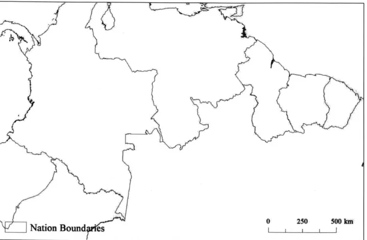
A geospatial data layer delineating national boundaries allowed for the disaggregation of the other global geospatial data layers into nation-level data. While the data could have been aggregated directly into the six C-ROADS regions, the disaggregation into nation-level data first allows for the capability to group the countries as future implementations of the model requires.

0 250 500k

Nation Bound

es

I

Despite their definition of various land uses, neither the IPCC nor FAO provide geospatial land area data associated with their categories. Consequently, land cover classes, for which geospatial data were available (Figure 4), were used as proxies for land use. These land cover classes, defined by vegetation and coverage characteristics, were mapped onto the IPCC land use categories (Table S3), and then C-ROADS land use categories (Table 1).

Figure 4. European Space Agencv and Climate Change Initiative land cover map depicted by 300m x 300mn pixels: Northern Amazon.

Recognizing that vegetation and biomass carbon intensity vary substantially across climatic domains, the distribution of these domains were accounted for within each country. This research uses the widely accepted FAO framework of climate domains - tropical, subtropical, temperate, boreal, and polar - and their constituent global ecological zones, or ecozones (Sirnons, 2001). (Figure 5 and Table S4)

!, a

~J

"m~~-~

Ad

j

desrt

Tropical dry forest

Tropical moist forest

Tropical mouMain-ySte

Tropical rdinforcst

Tropical shrubland

0 250

I i I 1 I

Figure 5. Global ecological zones within the tropical climatic domain: Northern Amazon.

500 km

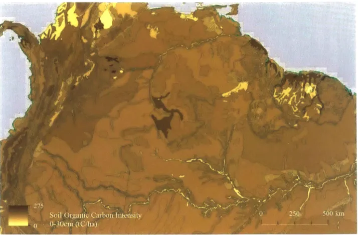
Soil carbon for each land use and region was derived from the Digital Soil Map of the World (DSMW) (FAO, 2003). The DSMW provides 'soil unit symbols' and their associated values for soil characteristics including the percentages of sand, silt, and clay in the topsoil (0-30cm) and subsoil (30-100cm), as well as the soil organic carbon (SOC) in both as a percentage of mass. 'Soil mapping units' consist of various compositions of particular soil unit symbols. DSMW polygons, p, are geospatial area vectors of each characterized by a single soil mapping unit. Only the topsoil (0-30cm) was used in this study in order to reflect the importance of this layer over the timeframe being studied. The SOC densities were bounded by a ceiling defined by the 9 5' percentile SOC intensity in order to control for outlier soil data and resultant over-estimation of soil carbon.

Permafrost SOC intensities were estimated using the Northern Circumpolar Soil Carbon Database version 2 (NCSCDv2). (Figure 7) As described by Hugelius et al. (2014), "the SOC stocks estimates for the 0-0.3 and 0-Im depth ranges were calculated separately in each NCSCDv2-region (i.e. Alaska, Canada, Contiguous USA, Europe, Greenland, Iceland, Kazakhstan, Mongolia, Russia and Svalbard) following the methodology of Tarnocai et al. (2009) but using the revised and gap-filled data sets described by Hugelius et al. (Hugelius, Bockheim, et al., 2013; Hugelius, Tarnocai, et al., 2013)."

Figure 7. Northern Circunmpolar Soil Carbon Daiahase \W IHn l

The coordinated projection of these geospatial data layers (Figure 8) allowed for disaggregation and attribution of data from one layer to another. Specifically, the tabulation of area of land cover class within soil polygons enabled the calculation of the soil organic carbon underlying different land uses. Similarly, area of land cover classes within polygons of different ecozones enabled the calculation of the

Figure 8. Layering of geospatial data: Northern Amazon. Top: nations, Second: land cover; Third: ecozones: Bottom: soils

Further-nore, nation-level land use areas were weighted by the coverage of climatic domains within each nation. While this assumes that the distribution of land uses across each domain is uniform within a nation, it nonetheless provides a higher degree of granularity for those nations with significant areas in multiple climatic domains, particularly the US, China, and India. This methodology builds upon that of Keenan et al. (2015), in which each country was assigned to the single climatic domain that held the most coverage within it.

2.2.2 Biomass Carbon Intensity

Biomass carbon intensities by land use and region were reconstructed from the New IPCC Tier-1 Global Biomass Carbon Map for the Year 2000 (GBCM) (Ruesch & Gibbs, 2008). The GBCM used the 2006 IPCC Guidelines for National Greenhouse Gas Inventories (IPCC, 2006) to estimate the biomass carbon intensity of land by land cover class, ecozone, and continental region - Africa, North America, South America, Europe, Continental Asia, Insular Asia, Australia, or New Zealand. As such, the biomass carbon intensities by land cover class, ecozone, and continental region were reconfigured to estimate biomass carbon intensities by land use and C-ROADS region.

First, biomass carbon intensities by land cover class, ecoregion, and continental region were averaged into their appropriate land use, climatic domain, and continental region (Table S3 and Table S4) The nation-level biomass carbon intensities were then constructed as the average of the appropriate continental region-level biomass carbon intensities, weighted by the coverage of each climatic domain within its national boundaries. Finally, the biomass carbon intensities for land uses by C-ROADS region were constructed as

the average of their constituent nation-level biomass carbon intensities, each weighted by the nation-level land use area as a fraction of the land use area within the C-ROADS region.

Each ecoregion and continental region had biomass carbon values for both frontier and non-frontier classes of vegetation, where 'frontier' is defined as "relatively unmanaged forests with little human disturbance" (Ruesch & Gibbs, 2008). Frontier and non-frontier values only differed for certain temperate, boreal, polar forest systems. For conservative estimates, only non-frontier values were used. The resulting biomass carbon intensities were used for all land uses except for the Forest types, for which FAO biomass carbon stock values and land areas were scaled up from the nation-level reported data.

2.2.3 Soil Carbon Intensity

Soil carbon intensities by land use and region were constructed from the DSMW, ESA/CCI Land Cover, and national boundary geospatial layers. First, the soil bulk densities of specific soil symbol units were constructed as the weighted average of the densities of sand, silt, and clay, according to their fractional composition of the soil symbol unit (Walter, Don, Tiemeyer, & Freibauer, 2016). Second, SOC intensities of soil symbol units were constructed as the product of the soil bulk densities and the organic carbon percentage for the specific soil unit elements. Third, SOC intensities of soil mapping units were constructed as the weighted average of their component soil unit elements. Fourth, nation-level SOC intensities of soils underlying specific land uses were constructed as the average of the soil mapping unit SOC intensities, each weighted by the fraction of the specific land use coverage within a specific polygon relative to the total specific land use coverage within all the soil mapping unit polygons in the country. Finally, C-ROADS region land use SOC intensities were constructed as the average of the nation-level land use SOC intensities, each weighted by the nation-level land use areas.

The soil carbon intensities of permafrost land use by region were constructed from NCSCDv2. Some of the pedons (soil samples) used to construct NCSCDv2 were overlain by forest vegetation. To prevent overlapping and consequent double counting of soil carbon under land uses, permafrost was constrained to be only that land area that was covered in tundra vegetation in addition to being underlain by gelisol, or permafrosted, soils (Hugelius, Tarnocai, et at., 2013; USDA, 1999). ESA/CCI land cover classes 140, 150,

15 1, 152, and 153 - including mosses and lichens, and sparse vegetation (tree, shrub, herbaceous cover), respectively - were used to delineate tundra land cover. SOC intensity values by NCSCDv2 polygons were weighted by fractional tundra cover and fractional composition. Because the land cover classes used for tundra fell under the other land category of FAO, the soil stocks and areas of permafrost land use were

subtracted from those of other land use to prevent double counting of the permafrost carbon and land. 2.2.4 Land Uses

2.2.4.1 Forest

The forest parameters were estimated differently than those of the other land uses due to the importance of the qpAB, K, and v parameters for forests in particular, as well as the availability of forest growth curves. The time series profiles of biomass carbon intensity and soil carbon intensity of land as specific tree species grew from seedlings or planting (Smith, Heath, Skog, & Birdsey, 2006) were used to estimate the individual forest parameters with the simultaneous optimization of parameters methodology used by Sterman et al. (2018). Tree species were then mapped into domain-level forest types - temperate, subtropical, and boreal. (Table S5) Due to the high degree of nonlinearity between the parameters within a specific forest system, the median value of each optimized parameter for each domain-level forest type was used to represent the

domain-level forests in order to reduce the influence of outlier parameter values. Parameter estimates for tropical forests were optimized using a similar optimization method, albeit with tropical forest carbon growth curves constructed from individual tropical tree growth curves and tropical forest tree density estimates (Glick et al., 2016; Kbhl, Neupane, & Lotfiomran, 2017). Further detail on the estimation process for tropical forests can be found in the Appendix. The presence of multiple climatic domains per country, especially for larger countries with significant forest area in multiple domains, necessitated the weighted averaging of the forest type parameters to obtain C-ROADS region forest parameters.

2.2.4.2 Harvested Forest

The parameters for C-ROADS region forests were used for harvested forests. 2.2.4.3 Cropland

The equation used to represent NPP on cropland was simplified to reflect its relatively simple growth pattern relative to that of forests. Specifically, cropland biomass growth is less sensitive to the current state of the crop, allowing pAB = 0, and the Richards shape function is less important for the significantly lower biomass carbon intensity of croplands, allowing v = 1. Under these assumptions, Equation (2) becomes:

NPPu,r = Ku,r (B*u,r - Bu,r) (4)

Furthermore, KAB for cropland is large compared to that of forests. Assuming that crops reach maturity, approaching 95% their equilibrium state, within one year sets K AB= 3 yr-1. Additional considerations on this assumption can be found in the Appendix.

Harvest in is research pertains only to the harvest of forest for wood bioenergy and does not appear in the

cropland formulations. Rather, the crop harvest is contained within the tern Bu,rPuA from Equation (1). The total nation-level flux of carbon from biomass to atmosphere on croplands was taken to be the combined carbon contained within harvested crop biomass and the crop residues produced during the crop harvesting process, summed for each crop of that country.

BAi = CPi * C + CRi * Cce (5)

CRi = CPi * RPi (6)

BAi is the carbon flux of a particular crop, CPi is the crop production or amount of biomass harvested (FAO,

2018), C is the carbon content of the harvested portion of the crop (Monfreda, Ramankutty, & Foley, 2008),

CRi is the crop residue of the particular crop, and Cceii is the carbon content of the residue (Wolf et al.,

2015). CRi was formulated as the product of CPi and the residue production ratio, RPi, of the particular

crops responsible for the grand majority of the world's crop residues (R Lal, 2005). The crop production (kg) of 161 unique crops in 216 countries in the year 2016 were gathered from FAOSTAT (FAO, 2018). Average residue:crop production ratios for each crop residue type used were calculated from production and residue production numbers from 1991 and 2001 (R Lal, 2005). Theses nation-level fluxes were divided by the reported cropland area of each nation (FAO, 2018) to estimate the nation-level biomass to atmosphere carbon flux intensities.

The total nation-level flux of carbon from biomass to soil was calculated as the belowground biomass carbon for those crops that also produced residue, under the assumption that not all crops (ex: fruit trees) produce significant annual residue and their roots do not become soil during the span of a year.

Contrastingly, crops that produce significant residues during harvesting and must be replanted with each growth cycle - including maize, millet, oats, etc. - were lose their roots and the carbon they contain to the soil between each harvest. These nation-level flux were divided by the reported cropland area of each nation (FAO, 2018) to estimate the nation-level biomass to soil carbon flux intensities.

The domain-level carbon flux intensities from soil to the atmosphere from the 2006 IPCC Guidelines for National Greenhouse Gas Inventories (IPCC, 2006). (Table S6)

2.2.4.4 Pasture

AB AR

The assumptions for p , V, K on croplands were also applied to pasture. Based on their geographic coordinates, 31 carbon flux measurement sites (Scurlock, Johnson, & Olson, 2002) were mapped into the FAO climatic domains, for which the average NPP was calculated for each. Individual NPPs were calculated via method 5 according to Scurlock et al. (2002). The carbon mass per dry matter (d.m.) mass was set to be 0.44 (g C [g d.m.]') under the assumption that the carbon mass per dry matter mass of pasture

land is similar to that of agricultural roots and stocks (Wolf et al., 2015).

Domain-level carbon flux intensities from soil to atmosphere were based on the annual emission factors for drained grassland organic soils (IPCC, 2006). (Table S7) Domain-level carbon flux intensities from biomass to soil were assumed to equal those from soil to atmosphere values in equilibrium. Domain-level carbon flux intensities from biomass to atmosphere were calculated to be the difference between NPP and the carbon flux intensities from biomass to soil, and were constrained to be greater than or equal to zero.

2.2.4.5 Permafrost

It was assumed for this model that permafrost did not have active fluxes.

2.2.4.6 Other

It was assumed for this model that other land did not have active fluxes from biomass to atmosphere or from biomass to soil. Fractional parameters for carbon flux from soil to atmosphere were calculated directly from the annual change in organic carbon stocks in mineral soils with a time dependence of stock change factor of 20, as recommended for Tier 1 calculations for soils on other land (IPCC, 2006).

2.2.5 Fractional Flux Parameterization

Each of the input parameters to NPP, as well as those to the carbon flux from biomass to soil, biomass to atmosphere, and soil to atmosphere (Table 2), were estimated for each land use and region.

Table 2. Parameters of interest, specific to land use, it, and region. r

Parameter Units Definition

pBj yr- Reference rate of C flux from atmosphere to biomass in Richards function for NPP, by land us and region

pr yrI Fractional rate of C flux from biomass to atmosphere, by land use and region

BS yr-I Fractional rate of C flux from biomass to soils, by land use and region

SP~r yr- Fractional rate of C flux from soils to atmosphere, by land use and region

B*ur tC [ha]-' Maximum biomass C intensity of the land, by land use and region

Kur yr- Rate of C flux from atmosphere to biomass proportional to max biomass in NPP model, by land use and region

Vu,r D'less Shape parameter in the Richards growth function for NPP

constructed by dividing the C-ROADS region flux intensities by their corresponding C-ROADS region biomass or soil carbon intensities. The flux intensities were reported in the literature or constructed from data in different scales: level, domain-level, or ecozone-level. (Table S4) If obtained at the nation-level, the C-ROADS regional flux intensities were constructed by taking the average of the nation-level intensities, weighted by their specific land use area as a fraction of the C-ROADS region specific land use area. The C-ROADS region flux intensities were then used to calculate the fractional flux parameters. If obtained at the domain-level, the nation-level flux intensities were constructed by taking the average of the domain-level intensities, weighted by the climate domain coverage within the nation. The nation-level intensities were then used to construct the C-ROADS regional flux intensities, etc. If obtained at the level, the domain-level flux intensities were constructed as the average of the reported ecozone-level intensities, etc.

With the fractional flux parameters estimated, the maximum biomass carbon intensity of the land,

B*, can be calculated. Assuming that the biomass carbon intensities estimated previously represent the

vegetation in their respective states of equilibrium, combining Equations (1) and (2) gives:

BrBS BA

B*ur - Bu,rrur + BuruPr + Bu,r (7)

Ku,r

2.3

Simulations were run from a state of equilibrium to allow a clearer interpretation of the highly interconnected dynamics at play. Equilibrium biomass intensities from which to initialize the stocks of the model were found individually for each land use and region. However, due to the magnitude of the global behavior over which these parameters have influence, upon importing these initial carbon intensities into the model, rounding errors produced a slight disequilibrium that affect the base case scenario. As such, the atmospheric concentration of carbon increases approximately 0.01 ppm over the course of a century in the base case. (Figure 9)

Change in [CO2]

.1

0-.05

-20 0 20 40 60 80 100

Delta Atm C02 Concentration: Base

Figure 9. Base Case illustrates computational constraints to achieving pure equilibrium starting conditions.

Nevertheless, despite the dynamic carbon fluxes between biomass, soil, and atmosphere, over each land use, between each global region, over time, the total carbon in the global system modeled is conserved. (Figure 10) Total C 3.07 M 3.065 M S3.06 M 3-055 M 3.05 M -20 8 36 64 92 120 148 176 Year

Total C Bio Soil Ocm Atmoepht. Foul plo. CH4 :aw

Figure 10. Conservation of global carbon mass across all stocks over time.

The extended model conserved land area and total carbon throughout the system for all of the LULUCF scenarios simulated. The full list of model equations, their units, and accompanying comments are documented in the appendix.

3

RESULTS

3.1

The behavior of a single pulse of end use bioenergy demand is simulated. This means that enough Forest to provide the appropriate fuel to satisfy the demand - accounting for the fraction of clearance during harvesting, land availability, combustion efficiency, and processing efficiency, each of which are fully interactive variables for rapid testing of assumptions - is harvested and converted to harvested forest. A 10e+9 GJ end use bioenergy pulse, and its offset of energy generation of a customizable fossil fuel source for which coal was used here, is simulated at time step=0. This simulation also conservatively assumes that the land is thinned with a 0.25 fraction of biomass removed from harvested land by bioenergy harvest.

Total Flux to Atmosphere

10

Total Flux Biomas and Soil to Aim region r[US] : US.BioEa(le-10)

Flux Atm to Blomas mglon rUS] : US.BioBEl*+l0) Total Flux Biomass ad Soil to Atm regiona USJ: Base Flux Atm to Biomass rgon: Barn

Figure 11. End use bioenergy pulse releases carbon to the atmosphere. Blue: bioenergy pulse case.

The total flux of carbon into the atmosphere is greater than the base scenario - even when offsetting the combustion of coal - due to lesser combustion and processing efficiencies of wood bioenergy as compared to coal. Wood holds more moisture than does coal, and some of the energy that would have been used to generate useable energy during combustion is immediately dissipated by the evaporation of that moisture (Sterman et al., 2018). Additionally, the processing losses associated with the wood pellet processing and supply chain are greater than those associated with the supply chain of coal (Baruya, Mcculloch, & Ewart, 2012; R6der, Whittaker, & Thornley, 2014).

-

-,-- - I

Change in [C02]

"."

""....

I

Delta Atm C02 COceatrati: US BioEn(.10)

Delta Atm C02 Concntrati: Base

Figure 12. The increased atmospheric concentration of C02 decreases over thne due to re-sequestration of carbon into growing bionass. Blue: bioenergv pu/se case. Red: base case.

As the Harvested Forest regrows to its stable equilibrium, it removes carbon from the atmosphere until the concentration of carbon dioxide in the atmosphere drops below that of the base case after a period of 24 years. This is termed the payback period.

US Land Type

LaadAseeu 4FbnatUSjUS.Bb(1e+10) e... L&d Am u 4Hrted FeetUSJ: U.In(le10) ...-...

Figure 13. US forest to harvested forest conversion in bioenergy pulse case. Blue: forest area. Red: harvested Ibrest area.

US C in Biomass

Biomnun C Lnd Unu Region 4(Fomet,US): USBAia~n(I&#,I) - - e ese e

Bioams C Lmd Use u Rqiom HWvwd Fomst,US): USBio1e1O) -a-

-Figure 14. Stacked representation of the carbon stock in forests and harvested Iorests of the US in bioenergv pulse case. Blue: carbon infbrest. Red: carbon in harvested fbrest.

The Fraction of Biomass Removed for Bioenergy of 0.25 dictates the portion of biomass carbon that was not transferred to the Harvested Forest stock, but was instead released into the atmosphere for bioenergy supply. (Figure 14)

Unit NPP

I

NPP per IFcerest,US1: USBioB*..+10) NPP per xr(Hrv.u FoeUS) : US.Bio*EI&+10)

Figure 15. NPP per unit area for bioenergv pulse case. Blue: fbrest. Red: harvested Jfrest

For low harvest fractions, NPP of the Harvest Forest begins at a higher rate than the steady-state Forest because, as detailed in the Richards formulation in Equation (2), it has room to grow before the approach of the maximum biomass carbon intensity produces a strong enough balancing feedback to reduce the NPP into equilibrium.

3.1.1 Harvest Fraction

Harvest often consists of clear-cutting the grand majority of a forest's biomass down. A fraction of biomass carbon removed from harvested forest for bioenergy of 0.95 was used to simulate the effect of clear-cutting scenarios.

Figure 16 Stacked representation ofthe carbon stock in forests and harvested forests of the US in

clear-cut. Blue: carbon in forest. Red: carbon in harvested firest.

bioenergy pulse case with 95%

Both methods release the same amount of carbon at the pulse because the land area is scaled to inversely with harvest fraction to achieve the same end use bioenergy supply. (Figure 14 and Figure 16)

.4 -2 0 .4

Change in [C02]

Deta Atm C02 Comuenation: USBioW(+10)uHWu(95) Delta Atm C02 Concaurtimn US.BioN(1e10)

Deit Atm CO2 Concnation: Base

Figure 17. Change in atmospheric C02 concentration. Green: base case.

Red: harves tead irest fi-om thinning (harvest fraction = 0.25) Blue: harvested forest fron clear-cut (harvest fraction = 0. 95)

US C in Biomass

Bioman C Land Use Region 4Formt,US: US.Bion(e+10)HWac(95) e e en

However, not only does clear-cutting for bioenergy harvest release carbon into the atmosphere, as thinning also does, but it also takes away its capability to recapture that carbon quickly. The thinned harvested forest has enough biomass left on its land that it exhibits a higher NPP at the outset, allowing it to move towards its equilibrium quickly. Clear-cut land, on the other hand, starts with significantly less biomass carbon intensity with which to reabsorb carbon fi-om the atmosphere. These dynamics can be seen in the second derivatives of atmospheric concentration or the values of unit NPPs of Harvested Forest scenarios. (Figure 17 and Figure 18)

Unit NPP for Harvested Forest

I

/

4OR

NPP pr ara(Hveted Foeat,USI: USBioEn(Ie-l0)_WFtac(95)

NPP per e(Hervswed Foet,USj: USBAoi1eV+lO) NPP per mem(Harvested Foet,US): Base

Figure 18. NPP per unit area of/harvested fbrest. Green: base case. Red: thinned. Blue: clear-cut.

US C in Soil

Soil C Land Use u Region FomtUS): US_Bion(le+10)_HFc(95).-

e...ee-Soil C Land Use u Region [Haveted Fot,USJ: USBioE,~le+1O)_ac(9S5)

-Figure 19. Soil carbon inforest and harvested forest in bioenergy pulse case. Blue: soil carbon in forest. Red: soil carbon in harvested Ibrest.

_j

Forest harvest also has significant effects on the dynamics of soil carbon. (Figure 19.) Upon clear-cutting of a forest, there is no more tree litter providing the input to the stock of soil carbon, yet the soil is still providing outgassing of its current soil carbon. The soil carbon drops in for that converted land until the trees grow back and increasingly provide litter to the soil again.

3.1.2 Harvest Region

The composition of tree types varies significantly across the six C-ROADS regions. As such, regions exhibit different shapes of harvested forest regrowth and produce different patterns of carbon flux between the land and atmosphere.

Change in [C02]

Dim AtM CO2 CO.M.m OdMDWtfqgBWE1(c+10) Dim Atm C am r..mM. OdMauDidBiEdW1e+10) Ditm Atm CO2 Cu..moim: U.-UBiOW.+1% Dia Alm C02 Cunc.m.M.l CbmBiaLae+10)

Ditm AtM CO2 Cm.maa.. dIa.iBiOWI(*+1e4.1O

Date AtM C2 Cnc.m~Ma.. USBI(1+1)

Dd At. C02 Ce0.m03. BEW

Figure 20. Change in atmospheric carbon concentration on bioenergv provided fom firests of different regions.

Light blue: base case (no harvest) Brown: US. Black: India. Gray China. Green: EU. Red: other developed nations. Blue: other developing nations.

The regions with the highest percentage of tropical climate coverage exhibit the longest payback times. For India, clear-cutting a harvested forest results in a modeled payback time of 186 years. The lower end of the range for clear-cut forest was exhibited by China with a payback time of 42 years.

3.2 CONVERSION OF FOREST TO CROPLAND AFTER HARVEST FOR BIOENERGY

Change in [C02]

DIta Atm C02 Cocmacmio: USFaustko.Ctupluni

Delta Atm C02 Concenuauin: Bm

60 80 100

Figure 21. Using land for agriculture after clearcutting for bioenergv precludes the regrowth olfsuficient bionass.

Blue: Jbrest to cropland conversion after harvestfbr bionass. Red: base case.

Necessary, but not sufficient, for the logic of carbon-neutrality to apply to wood bioenergy, the harvested forest must be allowed to grow back to its full pre-harvest stand. If it is converted to any other land use, it cannot recapture the carbon it released in new tree growth. Conversion to cropland exhibits a sudden reuptake of a very small fraction of the release carbon due to the modeled fast growth of annual crops on the converted land. (Figure 21.) Nevertheless, the change in atmospheric carbon concentration continues to rise at a greater clip than the base case due to residual soil carbon release.

-j

50

-20 8 36 64 92 120 148 176

Year

Sel C Ltni U,. a RIon 4Ptst,USJ: USsIe.M.C.op~md a.. a... Soil C LA Un 0 PAio= jCOplMdUS: US.7Ko.jqCplnd...

Figure 22. Soil in the converted cropland releases the organic carbon it accumulated as forest soil.

Blue: Ibrest soil carbon Red: cropland soil carbon.

3.3

The effect of afforestation on atmospheric carbon concentration varies by region in which it takes place, as well as the land use that is being converted to new forest. The scenarios modeled here represent a linear increase in afforested area, such that a goal area of 1 OMha is converted from a chosen land use source is achieved at time step=40, with the afforestation starting at time step=10.

Change in [C02]

.1

Dft Am CO2 COMneMMK UIjSIbaepLOnd-AP

Delt AM CO COmla.:- RUjft Qep&.AF Dfat Alm C02 CmcnmEa1- COhAs.1.M.CnPhad.AF

Dela Aum C02 Cemman: nia1OMm..CuppldAF

Dlta Atm CO2 Cmm:n- ODO_10hCop1ndAF

Dela Am C02 COcmMgM- ODiWNjQu.1 Cpld.AF

Ddt Am C02 Cncaun: mBa.

Figure 23. Change in atmospheric carbon concentration due to JOMha of afforestationfroin cropland in different regions. Light blue: base case (no harvest). Blue: US. Red: EU Green: China. Gray: India. Black: other developed nations. Brown: other

developing nations.

US C in Soil

Afforestation in the regions with the most tropical climate coverage exhibits the greatest downward effect on atmospheric carbon concentration. Additionally, it matters more, from a climate standpoint, where the afforestation occurs as opposed to the land use being replaced. That is to say, the scale of impact that there is a greater difference between forests in different climate regions than there is between the croplands and pastures within a given region.

Change in [C02]

7--

Dela Aim C02 Caw i W-: HUOMh.PMwe.AF

Deia Aim C2 COMMhzia- Chis.@Mi.Pat=e..AF DeiS Aim C02 Ce tio.- IdiajOthePutORAF

Dela Aim C02 Co.mia.- ODOMhe.Ptwe.AF

Dela Atm C02 C*aac- ODi1gN_1IMbqPaytW AF Deta Aim CO2 CeQMna1iaa Be

Figure 24. Change in atmospheric carbon concentration due to JOMha of affbrestation fom pasture in difflrent regions. Light blue: base case (no harvest). Blue: US. Red: EU. Green: China. Gray: India. Black: other developed nations. Brown: other

4

DISCUSSION

This work supports the basic patterns of forest harvest for bioenergy, as well as the conversion of forest to other land use after harvest for bioenergy, identified by Sterman et al (2018). Furthermore, afforestation scenarios using either cropland or pasture for afforestation are observed to have largely similar outcomes. It is apparent from a longitudinal sample across the different scenarios simulated, with India and Other Developing Nations standing out in particular, that the majority climate domain present in each of the regions, which is to say, the type of forest being developed, is a major driver of this behavior.

This emphasizes the criticality of robust forest parameterization. The NPP parameters are extremely sensitive and nonlinear, and may be significantly impacted by the methods by which they are aggregated into climate domains and regions. Examination of different methods of parameter aggregation for retaining the unique nonlinear interactions between the variables is an area of future work. Furthermore, the forest growth profiles gathered from Smith et al. (2006) measured forests grown from seedlings or planting of young trees, whereas the forest growth profiles for tropical forest were constructed from individual tree growth profiles (Kohl et al., 2017) from trees that may or may not have grown in the presence of full tree stands. Environmental conditions of the tropical trees (shade from already grown tree canopies, etc.) may have affected the time it took for the measured trees to reach maturity, and thus affected the resulting parameters.

Other aspects of model parameterization that could be considered further include the data sources used. Values for crop-specific carbon content per unit of dry mass are available (Wolf et al., 2015) and may be used in the place of the single constant used in this research (Monfreda et al., 2008). Updated geospatial ecozone areas are available (Food and Agriculture Organization of the United Nations, 2012a, 2012b). However, corruption of vector geometries in the source file made it unusable for this analysis. Finally, the use of ecozone distribution within countries would provide another level of granularity untapped by the use of the aggregated climatic domains used in this model. However, as with all models, a trade-off must be made between form and function.

The challenge of rectifying land use and land cover definitions is explicitly acknowledged in the literature. Verburg, Neumann, and Nol (2011) explicitly identify the inconsistency between definitions and data selection and handling as particularly challenging. Significant effort was expended in attempt to align as closely as possible the various definitions of the land uses and land covers explored here, aggregating and disaggregating the data in a manner meant to minimize definitional inaccuracies, while conserving total land area. More explicit mapping between land uses and land coverage categories would not only make integrated earth system models more consistent with physical reality, but would also provide a more grounded basis with which to compare different models and facilitate useful communication between the realms of science and policy (Verburg, Neumann, and Nol, 2011). These challenges are no less apparent for land use and land cover change, especially in the context of modeling global carbon flux estimates in integrated earth system models (J Pongratz, Reick, Houghton, & House, 2014). Looking forward, a framework for the definitional mapping of land management practices that take place on single land uses, will become crucial as such land management is increasingly integrated into earth system models (Erb et al., 2017; Julia Pongratz et al., 2018).

5

CONCLUSION

There exist knowledge controversies for countless issues at the contested boundaries between science and policy. Such controversies are particularly difficult to tease apart when they pertain to large and complex socio-technical systems, let alone those that carry with them heavy political, social, and moral ramifications. The debate around wood bioenergy "carbon-neutrality" is one such controversy where lack of knowledge, lack of understanding, and the differences in the definitions of particular boundary objects converge to promote skewed mental models.

This work expands the C-ROADS land use model to incorporate six major land uses within six major global regions. Multiple granular global geospatial data sets were collated to derive a highly disaggregated data set of biomass and soil carbon intensities for land uses across countries and climatic domains. This was used to estimate model parameters pertaining to the carbon fluxes within and between the biosphere and the atmosphere.

While wood bioenergy can eventually result in net atmospheric carbon reduction when displacing coal, the initial increase of atmospheric carbon above that which coal would have produced creates a carbon debt that can take decades to repay, decades during which the increased atmospheric carbon could potentially spur irreversible climate dynamics. Forest harvest for bioenergy exhibited carbon payback times ranging from 20 to 186 years, depending on the region in which the harvest occurred and whether the forest was clear-cut or thinned. This assumes that the harvested forest was allowed to regrow to its full pre-harvest equilibrium state. In scenarios where the forest was converted to cropland after harvest, not only did atmospheric carbon increase permanently from the combustion of the wood, but the flux of carbon from the soil to the atmosphere increased due to the higher fractional rate of carbon flux from soil to atmosphere of cropland soils as opposed to that of forest soils. Afforestation was shown to remove carbon from the atmosphere, and simulations revealed that it was most effective in regions that had more tropical climate coverage.

The globally consistent integrated earth system model presented here enables the explicit dynamics embedded in a range of region specific LULUCF policies to be simulated in real-time and their climatic effects evaluated. As such, this work hopes to facilitate more intelligent climate-related goal setting and a greater appreciation for the unintended consequences of under-informed policy creation.

6

REFERENCES

Baruya, P., Mcculloch, S., & Ewart, D. (2012). Losses in the coal supply chain. Retrieved from https://www.usea.org/sites/default/files/122012_Losses in the coal supply chain ccc2I2.pdf Boettcher, M., Bontemps, S., Brockmann, C., Defourny, P., Kirches, G., Lamarche, C., ... Wevers, J.

(2015). Land Cover CCI -Product User Guide -Version 2.0. Retrieved from http://maps.elie.ucl.ac.be/CCI/viewer/download/ESACCI-LC-Ph2-PUGv2_2.0.pdf

Clark, D. A., Asao, S., Fisher, R., Reed, S., Reich, P. B., Ryan, M. G., ... Yang, X. (2017). Reviews and syntheses: Field data to benchmark the carbon cycle models for tropical forests. Biogeosciences,

145194, 4663-4690. https://doi.org/10.5194/bg-14-4663-2017

Cornwall, W. (2017). The burning question. Science (New York, N. Y), 355(6320), 18-21. https://doi.org/10.1 126/science.355.6320.18

Deng, L., Zhu, G.-Y., Tang, Z.-S., & Shangguan, Z.-P. (2016). Global patterns of the effects of land-use changes on soil carbon stocks. Global Ecologjy and Conservation, 5(5), 127-138. Retrieved from http://www.sciencedirect.com/science/article/pii/S2351989415300226

Erb, K.-H., Luyssaert, S., Meyfroidt, P., Pongratz, J., Don, A., Kloster, S., ... Dolman, A. J. (2017). Land management: data availability and process understanding for global change studies. Global Change

Biology, 23(2), 512-533. https://doi.org/10. 1111 /gcb.13443

ESRI. (2008). ArcGIS Desktop 9.3 Help. Retrieved from

http://webhelp.esri.com/arcgisdesktop/9.3/index.cfin?TopicName=Choosing a-map projection European Commission. (2015). Global Land Cover 2000 -Legend. Retrieved from

http://forobs.jrc.ec.europa.eu/products/glc2000/legend.php

Fiddaman, T., Siegel, L. S., Sawin,-E., Jones, A. P., & Sterman, J. (2017). C-ROADS SIMULATOR REFERENCE GUIDE. Retrieved from

https://d168d9ca7ixfvo.cloudfront.net/wp-content/uploads/2017/11/C-ROADSReferenceGuidev80.pdf

Food and Agriculture Organization of the United Nations. (2003). The Digital Soil Map of the World. Retrieved from http://www.waterbase.org/data/GlobalSoilData/readme.pdf

Food and Agriculture Organization of the United Nations. (2012a). Global Ecological Zones (second edition) (GeoLayer). Rome. Retrieved from http://ref.data.fao.org/map?entryld=2fb209d0-fd34-4e5e-a3d8-a 1 3c241 eb6 I b&tab=metadata

Food and Agriculture Organization of the United Nations. (2012b). Global Ecological Zonesfor FAO

Forest Reporting: 2010 Update (No. 179). Retrieved from http://www.fao.org/3/a-ap86 1 e.pdf

Food and Agriculture Organization of the United Nations. (2018). FAOSTAT. Retrieved from http://www.fao.org/faostat/en/#hone

Glick, H. B., Bettigole, C., Maynard, D. S., Covey, K. R., Smith, J. R., & Crowther, T. W. (2016). Data Descriptor: Spatially-explicit models of global tree density. Nature Scientific Data.

https://doi.org/10.1038/sdata.2016.69

Houghton, R. A., & Nassikas, A. A. (2017). Global and regional fluxes of carbon from land use and land cover change 1850-2015. Global Biogeochemical Cycles, 31(3), 456-472.