HAL Id: hal-00296414
https://hal.archives-ouvertes.fr/hal-00296414
Submitted on 18 Jan 2008
HAL is a multi-disciplinary open access
archive for the deposit and dissemination of
sci-entific research documents, whether they are
pub-lished or not. The documents may come from
teaching and research institutions in France or
abroad, or from public or private research centers.
L’archive ouverte pluridisciplinaire HAL, est
destinée au dépôt et à la diffusion de documents
scientifiques de niveau recherche, publiés ou non,
émanant des établissements d’enseignement et de
recherche français ou étrangers, des laboratoires
publics ou privés.
stratosphere
R. Müller, J.-U. Grooß, C. Lemmen, D. Heinze, M. Dameris, G. Bodeker
To cite this version:
R. Müller, J.-U. Grooß, C. Lemmen, D. Heinze, M. Dameris, et al.. Simple measures of ozone depletion
in the polar stratosphere. Atmospheric Chemistry and Physics, European Geosciences Union, 2008, 8
(2), pp.251-264. �hal-00296414�
www.atmos-chem-phys.net/8/251/2008/ © Author(s) 2008. This work is licensed under a Creative Commons License.
Chemistry
and Physics
Simple measures of ozone depletion in the polar stratosphere
R. M ¨uller1, J.-U. Grooß1, C. Lemmen1,*, D. Heinze1, M. Dameris2, and G. Bodeker3
1ICG-1, Forschungszentrum J¨ulich, 52425 J¨ulich, Germany 2DLR, IPA, Oberpfaffenhofen, Germany
3NIWA, Private Bag 50061, Omakau Central Otago, New Zealand
*now at: Copernicus Instituut voor Duurzame Ontwikkeling en Innovatie, Universiteit Utrecht, 3584CS Utrecht, The
Netherlands and Institut f¨ur K¨ustenforschung, GKSS-Forschungszentrum Geesthacht GmbH, 21502 Geesthacht, Germany Received: 15 May 2007 – Published in Atmos. Chem. Phys. Discuss.: 6 July 2007
Revised: 16 November 2007 – Accepted: 5 December 2007 – Published: 18 January 2008
Abstract. We investigate the extent to which quantities that are based on total column ozone are applicable as measures of ozone loss in the polar vortices. Such quantities have been used frequently in ozone assessments by the World Meteo-rological Organization (WMO) and also to assess the perfor-mance of chemistry-climate models. The most commonly considered quantities are March and October mean column ozone poleward of geometric latitude 63◦and the spring min-imum of daily total ozone minima poleward of a given lati-tude. Particularly in the Arctic, the former measure is af-fected by vortex variability and vortex break-up in spring. The minimum of daily total ozone minima poleward of a particular latitude is debatable, insofar as it relies on one single measurement or model grid point. We find that, for Arctic conditions, this minimum value often occurs in air outside the polar vortex, both in the observations and in a chemistry-climate model. Neither of the two measures shows a good correlation with chemical ozone loss in the vortex de-duced from observations. We recommend that the minimum of daily minima should no longer be used when comparing polar ozone loss in observations and models. As an alter-native to the March and October mean column polar ozone we suggest considering the minimum of daily average total ozone poleward of 63◦equivalent latitude in spring (except for winters with an early vortex break-up). Such a definition both obviates relying on one single data point and reduces the impact of year-to-year variability in the Arctic vortex break-up on ozone loss measures. Further, this measure shows a reasonable correlation (r= − 0.75) with observed chemical ozone loss. Nonetheless, simple measures of polar ozone loss must be used with caution; if possible, it is preferable to use more sophisticated measures that include additional informa-tion to disentangle the impact of transport and chemistry on ozone.
Correspondence to: R. M¨uller ([email protected])
1 Introduction
Since the early eighties, substantial chemical ozone loss has occurred during winter and spring each year in the Antarc-tic (e.g., Jones and Shanklin, 1995; Tilmes et al., 2006; Huck et al., 2007; WMO, 2007); substantial chemical loss of ozone has likewise been reported for recent cold Arctic winters (e.g., Manney et al., 2003; Tilmes et al., 2004; WMO, 2007). In the very cold Arctic winter of 2004/05, the chemical loss of ozone came closer to Antarctic values (Manney et al., 2006; Rex et al., 2006; Tilmes et al., 2006; von Hobe et al., 2006; Jin et al., 2006). Sophisticated methods have been developed to separate dynamically induced changes of po-lar ozone from chemical ozone depletion (e.g., Proffitt et al., 1990; Manney et al., 1994; M¨uller et al., 1996; Rex et al., 2002; Harris et al., 2002; Tilmes et al., 2004; Christensen et al., 2005; Goutail et al., 2005, and references therein), Furthermore, it has been shown (Rex et al., 2004; Tilmes et al., 2004, 2006) that the deduced chemical ozone loss is closely related to the potential for the formation of polar stratospheric clouds (PSCs).
However, these methods rely on rather comprehensive data sets that are not available for all winters of interest, particu-larly those before the 1990s. Simiparticu-larly, the necessary infor-mation for applying such sophisticated methods to simula-tions conducted with chemistry-climate models (CCMs) is often not available for archived model output (e.g., Austin et al., 2003; Eyring et al., 2006; Lemmen et al., 2006b).
Consequently, measures of chemical polar ozone deple-tion are commonly employed that rely solely on total col-umn ozone data (e.g., Newman et al., 2004; Bodeker et al., 2005; Huck et al., 2007). The two most frequently em-ployed measures are the average total column ozone in spring (March, NH and October, SH) poleward of 63◦and the min-imum of daily total column ozone minima over the polar cap (e.g., Newman et al., 1997; M¨uller, 2003; Austin et al., 2003; WMO, 2003; Shepherd, 2003; Eyring et al., 2006, 2007;
WMO, 2007). For assessments of the World Meteorologi-cal Organization (WMO) and of the Intergovernmental Panel on Climate Change (IPCC), the average March total column ozone poleward of 63◦N (Newman et al., 1997) has been reg-ularly used (WMO, 1999, 2003; IPCC/TEAP, 2005; WMO, 2007). The value of 63◦N was chosen by Newman et al. (1997), because “. . . the area poleward of 63◦N is [. . . ] large enough to contain the polar vortex, yet small enough to not be dominated by mid-latitude air masses in the lower strato-sphere”. Obviously, this condition will be better fulfilled in some Arctic winters than in others depending on the vary-ing size and shape of the polar vortex (Waugh and Randel, 1999; Karpetchko et al., 2005). And there are winters when the Arctic vortex breaks up before March (WMO, 2007).
The minimum of daily total ozone minima poleward of a particular latitude has been used as a standard to assess the performance of CCMs (e.g., Austin et al., 2003; WMO, 2003; Eyring et al., 2006, 2007; WMO, 2007). This measure is problematic, insofar as it relies on one single measurement or on one single model grid point. Knudsen (2002) criticised the use of this parameter and pointed out that the minimum ozone in the Arctic is frequently caused by high pressure sys-tems rather than by chemical ozone destruction. He therefore argued that, for example, the March mean total column ozone poleward of 63◦N would be a more suitable measure for the development of polar ozone.
Here, we scrutinise the information that can be deduced from simple (total column ozone based) measures of chemi-cal ozone loss and investigate circumstances where mis- and over-interpretations might occur. Our study uses a combined data set of satellite-based total column ozone measurements (Bodeker et al., 2005) from 1978 to 2007 (Sect. 2). Monthly mean column ozone poleward of 63◦ in spring (Newman et al., 1997; WMO, 2007) shows similar year-to-year vari-ability as vortex mean ozone, but neither of these quantities shows a close relation to meteorological quantities that de-scribe the potential for polar heterogeneous chlorine activa-tion and thus ozone loss (Sect. 3). Furthermore, we argue here that the minimum of daily total ozone minima poleward of a particular latitude should no longer be used when com-paring polar ozone loss between observations and CCMs be-cause this minimum value often occurs in air outside of the polar vortex (Sect. 3). As a better alternative for a total ozone based measure, we suggest using the minimum of daily aver-age total ozone poleward of a particular equivalent latitude in March or October. However, whenever possible, more sophisticated measures of chemical polar ozone loss should be used that allow the impact of transport and chemistry on ozone to be disentangled.
2 The total column ozone data set
The data set used here is version 2.7 of the NIWA combined ozone database which provides daily total column ozone
fields from November 1978 to March 2007. It is based on version 8 TOMS (Total Ozone Mapping Spectrometer) re-trievals from four different satellites (Nimbus 7, Meteor 3, ADEOS, and Earth Probe), total column ozone retrievals from the application of the TOMS version 8 retrieval al-gorithm to OMI (Ozone Monitoring Instrument) measure-ments, version 4.0 GOME (Global Ozone Monitoring Ex-periment) ozone retrievals, GOME total column ozone fields from the KNMI TOGOMI algorithm, and version 8 SBUV (Solar Backscatter Ultra-Violet) retrievals from four different satellites (Nimbus 7, NOAA 9, NOAA 11, and NOAA16). It updates the data set described in Bodeker et al. (2005), extending it to the end of March 2007, and implementing a number of improvements including:
– Data from both the Dobson spectrophotometer and Brewer spectrometer global networks are now used to remove offsets and drifts between the various satellite-based total column ozone data sets used to construct the database.
– Data from the Ozone Monitoring Instrument (OMI) flown onboard NASA’s Aura satellite since September 2004 are now used. Differences between OMI over-pass measurements and ground-based measurements are small (−2.8±5 DU) and the OMI grid data are cor-rected before they are combined with the other data sources, which are also corrected as in Bodeker et al. (2005).
– A better correction function for the Earth Probe TOMS ozone measurements has been derived to account for non-linearities in the drift between the Earth Probe TOMS measurements and ground-based measurements in recent years. Since September 2004 these data have only been used when OMI data are unavailable. – For the DLR GOME retrieval, a new data version (4.0)
was used and a better screening of anomalous ozone measurements at high solar zenith angles has been im-plemented. As the GOME 4.0 retrieval shows no bias against ground-based instruments (Balis et al., 2007), no corrections to these data were applied.
– In previous versions of the combined database, data from only one satellite-based instrument were used on any given day. In this version of the database, data from all satellite-based instruments are considered se-quentially to fill each 1.25◦ longitude by 1.0◦latitude
grid cell with a priority of Nimbus 7 TOMS, Meteor 3 TOMS, OMI, Earth Probe TOMS, ADEOS TOMS, the KNMI and then DLR GOME ozone retrievals, and then the 4 SBUV data sets. For example, if most, but not all, of the globe is covered by Nimbus 7 TOMS and Meteor 3 TOMS data are available to fill the gap, then these data are used for this. Both data sets, as before, are first corrected for offsets and drifts against the ground-based
measurements. In previous versions of the database however, only the Nimbus 7 data would have been used for that day and the gap in the data would remain.
3 Results
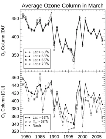
3.1 Mean total column ozone over the poles in early spring To test the sensitivity of the calculated Arctic mean ozone to the selected latitude limit, the March mean Arctic total column ozone for a latitude boundary at 63◦N, as originally chosen by Newman et al. (1997), is compared with the mean for boundaries at 60◦N, 65◦N, and 70◦N in Fig. 1 (top panel). Note that in some winters (1987, 1999, 2001, and 2006; WMO, 2007), Santee, 20081, the polar vortex broke
up in February; for those winters, the March mean total col-umn ozone hardly provides any information on polar ozone loss.
Clearly, the monthly spatial means are not very sensitive to the exact choice of the threshold latitude. A very similar pic-ture is found for the average total ozone column in April (see electronical supplementhttp://www.atmos-chem-phys.net/8/ 251/2008/acp-8-251-2008-supplement.zip). For the eight-ies, and in the warmer winters during the nineteight-ies, choos-ing a more poleward threshold latitude yields greater average ozone columns. The opposite (a smaller ozone column for a more poleward threshold latitude) is observed for the cold Arctic winters 1994/1995, 1995/1996, and 1999/2000 when substantial chemical ozone loss was observed (e.g., Manney et al., 2003; Tilmes et al., 2004). The strongest effect arising from changing the threshold latitude is found for the winter 1996/1997, a winter where the March mean column ozone showed an unusually strong meridional gradient (Newman et al., 1997).
Using equivalent latitude (8e) rather than geographic
lat-itude as an estimate of the boundary of the vortex (e.g., Butchart and Remsberg, 1986; Lary et al., 1995) should lead to a better demarcation between polar and mid-latitude air. Therefore, in Fig. 1 (bottom panel), the total column ozone average for March in the Arctic is shown using both the lat-itude and the equivalent latlat-itude poleward of 63◦N as the threshold. Here and throughout the paper equivalent lati-tude and other diagnostics of the vortex edge are evaluated on the 475 K potential temperature level. Overall the two av-erages show a similar inter-annual pattern. When equivalent latitude is used as the threshold, Arctic winters with a po-lar centric vortex (e.g., 1996/1997) show little change, while winters in the nineties with substantial chemical ozone loss within a perturbed vortex show lower averages. This result is
1Santee, M. L., MacKenzie, I. A., Manney, G. L., Chipperfield,
M. P., Bernath, P. F., Walker, K. A., Boone, C. D., Froidevaux, L., Livesey, N. J., and Waters, J. W.: A study of stratospheric chlo-rine partitioning based on new satellite measurements and model-ing, J. Geophys. Res., submitted, 2008.
Average Ozone Column in March
350 400 450
O3
Column [DU] Lat > 60oN
Lat > 63oN Lat > 65oN Lat > 70oN 1980 1985 1990 1995 2000 2005 320 340 360 380 400 420 440 460 O3 Column [DU] Lat > 63oN Φe > 63oN Nash
Fig. 1. Top panel: March mean Arctic total column ozone averaged poleward of 60◦N, 63◦N, 65◦N, and 70◦N. Bottom panel: March mean Arctic total column ozone averaged poleward of 63◦N com-pared with calculations using the equivalent latitude of 8e=63◦N
and the Nash criterion (applied on the 475 K potential temperature surface) as vortex edge definitions. All averages are area-weighted averages.
not surprising because, when using equivalent latitude as the threshold, the average ozone is less likely to be influenced by air from outside the vortex where, in winters with substantial ozone loss, ozone is higher. An estimate of the location of the vortex boundary, i.e. the location of the strongest barrier to meridional transport in the polar region which is based on fluid-dynamical theory, is the maximum gradient in potential vorticity in equivalent latitude constrained by the horizontal wind velocity (Nash et al., 1996). The edge of the vortex de-fined in this way agrees reasonably well with observed strong tracer gradients at the vortex boundary (e.g., Greenblatt et al., 2002; M¨uller and G¨unther, 2003). Because the area of the po-lar vortex varies substantially from year to year in the Arctic (e.g., Karpetchko et al., 2005; Tilmes et al., 2006), a constant equivalent latitude cannot provide an accurate estimate of the vortex area. Thus, because chemical ozone loss is confined to within the vortex boundary, it is expected that the average total column ozone poleward of the vortex edge as defined by Nash et al. (1996) should show lower values than an aver-age based on geometric or constant equivalent latitude. This
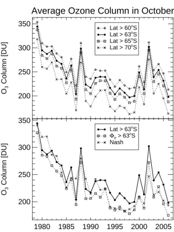
Average Ozone Column in October
200 250 300 350 O3 Column [DU] Lat > 60oS Lat > 63oS Lat > 65oS Lat > 70oS 1980 1985 1990 1995 2000 2005 200 250 300 350 O3 Column [DU] Lat > 63oS Φe > 63oS NashFig. 2. Top panel: October mean Antarctic total column ozone av-eraged poleward of 60◦S, 63◦S, 65◦S, and 70◦S. Bottom panel: October mean Antarctic total column ozone averaged poleward of 63◦S compared with calculations using the equivalent latitude 8e=63◦S and the Nash criterion (applied on the 475 K potential temperature surface) as vortex edge definitions.
is indeed borne out by the analysis, with the exception of the warm winters of 1978/1979, 1984/1985, 1987/1988, and 1998/1999 (Fig. 1, bottom panel). All four of these Arctic winters show a very low PSC formation potential and thus a very small potential for chemical ozone destruction (Rex et al., 2004; Tilmes et al., 2006). For all other winters, the polar average total column ozone using a potential vortic-ity gradient based threshold is lower than using any other threshold and the difference is particularly pronounced for winters showing strong ozone depletion. The sole exception is the winter of 1996/1997 that showed an unusually inhomo-geneous ozone distribution within the Arctic vortex with a particularly low ozone column in the vortex core (e.g., New-man et al., 1997; Manney et al., 1997; McKenna et al., 2002). The Arctic vortex, typically, is strongly eroded in April and is therefore smaller than the area encompassed by the 63◦N equivalent latitude contour (e.g., Waugh and Randel, 1999). Consequently, column ozone in April averaged over the vortex area as deduced using the Nash et al. (1996) crite-rion is expected to be lower than the average column ozone poleward of 63◦N equivalent latitude, as is the case here
(see electronical supplement, http://www.atmos-chem-phys. net/8/251/2008/acp-8-251-2008-supplement.zip). Because the Arctic vortex in April is unlikely to be polar-centred, computing a polar average column ozone using geomet-ric latitude rather than equivalent latitude as the thresh-old should lead to even more ozone-rich mid-latitude air masses being included in the average, and thus should lead to even greater averages as is indeed the case (see electronical supplement, http://www.atmos-chem-phys.net/ 8/251/2008/acp-8-251-2008-supplement.zip).
Although originally designed for the Arctic, the concept of the average total ozone column poleward of a threshold lat-itude of 63◦has been extended to the Antarctic, where Oc-tober mean values are commonly considered (e.g., WMO, 1999; IPCC/TEAP, 2005; WMO, 2007). In the Antarctic, the choice of the threshold latitude has a much stronger impact on the October average polar column ozone com-pared to the Arctic; the difference between a threshold of 60◦S and 70◦S is noticeable in every Antarctic winter anal-ysed here and can be as large as ∼50 DU (Fig. 2, top panel). The pattern of inter-annual change in the October mean ozone column, however, is not strongly affected by the choice of the threshold latitude. These statements are like-wise valid for the average total ozone column in September (see electronical supplement, http://www.atmos-chem-phys. net/8/251/2008/acp-8-251-2008-supplement.zip). As for the Arctic, the sensitivity of Antarctic average total column ozone to the latitude poleward of which the average is calcu-lated depends on the steepness of the meridional gradients in ozone across the vortex edge. For the latitude range consid-ered in Fig. 2, the ozone gradients are steeper in the Antarctic than the Arctic (see e.g. Fig. 5 from Brunner et al. 2006) and therefore Antarctic mean total column ozone is expected to be more sensitive to the spatial limiting latitude.
In the Antarctic, the 63◦S equivalent latitude contour is often located within the polar vortex in early spring (e.g., Bodeker et al., 2001, 2002). As a result, the difference between the average column ozone poleward of the Nash-defined vortex edge and the average poleward of 63◦S equiv-alent latitude (Fig. 2, bottom panel) is smaller than in the Arctic. Using the Nash vortex edge as the limiting contour for the averaging includes air masses towards the vortex edge that are not included if a threshold of 63◦S equivalent lati-tude is used. Because total column ozone in the Antarctic vortex increases towards the vortex boundary (Bodeker et al., 2002), using the Nash criterion will generally lead to greater polar total ozone averages (Fig. 2, bottom panel). The only obvious exception to this observation in the October time se-ries analysed here is the winter of 2002. In this winter, at the end of September, a sudden stratospheric warming oc-curred in the Antarctic vortex, leading to a much smaller and weaker vortex than usual, reminiscent of Arctic conditions (e.g., Kr¨uger et al., 2005; Newman and Nash, 2006).
March Minimum Ozone Column (>60o
N) Outside Polar Vortex
1980 1985 1990 1995 2000 2005 0 20 40 60 80 100 Percentage
Fig. 3. The fraction (in percent) of the daily total column ozone minima in the region 60◦N–90◦N occurring outside of the polar vortex in March. The polar vortex is defined here by the maximum gradient in potential vorticity (Nash et al., 1996).
3.2 Minimum column ozone in the polar region
3.2.1 Minimum polar total column ozone in observations Spatially localised and transient (several days) reductions in column ozone, so-called miniholes, are frequently observed; it has been established that they are of dynamical origin (McKenna et al., 1989; Petzoldt et al., 1994; James et al., 2000; Hood et al., 2001; Weber et al., 2002). The dynamics of miniholes involves a lifting of the tropopause above a tro-pospheric anticyclone and poleward motion of ozone-poor subtropical air in the upper troposphere and lower strato-sphere. In combination, this causes a reduction in column ozone (e.g., Reid et al., 2000; Hood et al., 2001). The dynam-ics of miniholes further results in equatorward excursions of polar air in the mid-stratosphere; in a situation where this air is chemically depleted in ozone by halogen chemistry in the polar vortex, particularly low ozone miniholes may occur (James et al., 2000; Weber et al., 2002; Keil et al., 2007). Fur-thermore, the frequency of low-ozone events changes with time; Br¨onnimann and Hood (2003) report that low-ozone events in winter were much more frequent in 1990-2000 than in 1952-1963 over northwestern Europe.
Nonetheless, the minimum of daily total column ozone be-tween 60◦and the pole for the period March/April in the Arc-tic and September-November in the AntarcArc-tic has been fre-quently employed as measure of polar chemical ozone loss for the validation of CCMs (Austin et al., 2003; WMO, 2003; Eyring et al., 2006, 2007; WMO, 2007). The minimum of daily total column ozone used in this study is defined as the minimum value of the daily minima over the respective pe-riods, i.e. one single measurement or one single model grid point within a two-month period.
In Fig. 3 it is shown that for winters with little chemical ozone destruction a substantial fraction of the daily mini-mum ozone columns occurs outside the polar vortex. For
March Minimum Ozone Column (Lat > 60oN)
1980 1985 1990 1995 2000 2005 200 220 240 260 280 300
Ozone Column [DU]
min of daily mins Lat > 60o
N Inside Vortex
Fig. 4. The minimum total column ozone in the Arctic poleward of 60◦N in March (solid line) computed as the minimum of daily minima. The dashed line shows the same calculation but excluding any minima occurring outside of the polar vortex. The polar vortex is defined here by the maximum gradient in potential vorticity (Nash et al., 1996).
half of the winters considered here about 50% of the daily minima occur outside of the vortex, and for only four win-ters is the fraction of minima occurring outside below 25%. Minima occurring outside of the vortex must be due to dy-namically caused low ozone events (see above) and cannot be linked with photochemical ozone loss in the polar vortex arising from heterogeneous activation of chlorine-containing molecules on polar stratospheric clouds.
If the minimum value of daily total ozone minima pole-ward of 60◦N (as used, e.g., in WMO, 2003, 2007) is com-puted, it provides information from within the polar vortex in only 12 out of the 29 winters considered here (Fig. 4). The deviation between the vortex minimum total ozone and the minimum total ozone poleward of 60◦N is significant, with a maximum deviation of ∼50 DU in the winter of 1984/1985.
In the Antarctic, because of the stronger reduction in col-umn ozone due to chemical ozone destruction, the situation is different. For the period considered here, the minimum of daily column ozone between 60◦S and the pole for the period September-November (not shown) is always located within the vortex.
3.2.2 Minimum column polar ozone in model results Differences between different simple measures of ozone loss and between simple and more sophisticated analyses also oc-cur when analysing results from model simulations, as will be shown below. Since the prediction of the recovery of polar ozone is based on simulations with CCMs (e.g. Austin et al., 2003; WMO, 2003, 2007; Eyring et al., 2007), the identifica-tion of a recovery period may depend on the analysis method-ology chosen for ozone loss. In the last two ozone assess-ments (WMO, 2003, 2007), the spatial minimum of the daily
250 300 350 400 450 Spatial Minimum Ozone Column (DU) 250
300 350 400 450
Spatial Mean Ozone Column (DU)
Vortex (1990) Polar cap
(1990)
Vortex (future) Polar cap (future)
Vortex (1990) Polar cap
(1990)
Vortex (future) Polar cap (future)
Fig. 5. Simulated 1 April total ozone column from two CCM 20-year ensemble (time slice) experiments with 1990 and near-future boundary conditions for greenhouse gases and sea surface temper-atures. For each time slice and for each analysis region (polar cap north of 60◦N, or vortex according to the maximum gradient in po-tential vorticity, Nash et al. 1996) the ensemble statistics of spatial mean ozone column are contrasted with those of the spatial min-imum ozone column. Each diagram indicates mean, range (solid lines), and one standard deviation (filled areas); quartiles are indi-cated as dotted lines centred around the medians which are shown as open diamonds.
spring ozone minimum poleward of 60◦served as a quanti-fier for the state of the polar ozone layer for comparison with simulations from different CCMs.
For simulated ozone columns, here we use as an exam-ple two time slice experiments from the chemistry-climate model ECHAM4.DLR(L39)/CHEM (hereafter abbreviated as E39/C Hein et al., 2001; Schnadt et al., 2002). Each ensemble experiment consists of 20 recurrent simulations with constant boundary conditions (sea surface temperature, greenhouse gases), one for the 1990s and one for the near-future. The near future conditions originally aimed at the year 2015, but in the interim it has been found that the sea surface temperatures used are too high. Therefore, results from the future simulation should not be considered as a re-liable projection of a specific period but rather as being in-dicative of possible future conditions. The 1990 time slice results, in contrast, are in agreement with the results derived from the most recent transient ensemble run for 1960 to 1999 (Dameris et al., 2005; Eyring et al., 2006). A detailed de-scription of both time slice experiments and the simulation of ozone therewith is given elsewhere (Schnadt, 2001; Lem-men, 2005).
Figure 5 compares ensemble statistics of both time slices analysed separately for the polar cap and the dynamically de-fined vortex, all data reported for 1 April. For example, in the
1990 simulation poleward of 60◦N (dark blue colour), the
spatial mean ozone column (ordinate) was 387 DU and the range was 310–439 DU. In half of the years, the spatial mean column was larger than 403 DU. For the same analysis, the mean and range of the spatial minimum column (abscissa) are 291 DU and 218–369 DU, respectively. Column val-ues for “future” (cyan, dark yellow) are consistently higher than for “1990” (blue, red) due to a lower chlorine loading and more dynamical heating leading to a stronger downward transport (Schnadt et al., 2002; Eyring et al., 2006).
For both time slices, the spatial mean total column ozone is higher over the polar cap than over the vortex, and the spatial minimum column is lower over the polar cap than over the vortex; this difference in spatial analysis is more pronounced in the future experiment (with less chemical ozone destruc-tion). For the 1990 experiment, 50% of the years have a mini-mum column of less than 310 DU analysed within the vortex, but 75% of these winters have a minimum column of less than 310 DU analysed within the polar cap. Evidently, for many years the minimum column ozone is located outside the vortex in spite of the, on average, lower ozone column within the vortex.
The erroneous association of the minimum column ozone with high chemical ozone loss becomes obvi-ous when chemical ozone loss deduced from methane-ozone tracer correlations (Lemmen, 2005; Lemmen et al., 2006b) is compared with minimum column ozone (see electronical supplement http://www.atmos-chem-phys.net/8/ 251/2008/acp-8-251-2008-supplement.zip for further dis-cussion). For all winters of both time slice experiments, the maximum chemical column ozone loss is located within (or, in two cases, on) the polar vortex edge. But only for three winters in each time slice experiment is the polar ozone min-imum located within the vortex. On the ensemble average, the vortex edge is located at 8e≈74◦±8◦in 1990 (78◦±6◦
for “future”), and the location of the polar cap minimum is around 62◦±15◦(57◦±13◦), i.e., clearly outside of the vor-tex.
Arguably, the simulated vortex area, 8e>74◦on 1 April
for many of the analysed winters is smaller than observed climatological Arctic vortex areas (e.g., Karpetchko et al., 2005, report 8e≈69◦ for the climatological Arctic vortex
edge for mid-March). The fact that the size of the Arctic vortex in E39/C is smaller than in reality is highlighted in the electronical supplement http://www.atmos-chem-phys. net/8/251/2008/acp-8-251-2008-supplement.zip, where the strength of the barrier to meridional transport is compared for analysed meteorological data and results from E39/C (Dameris et al., 2005) on the 550 K surface (averaged over the years 1990–1999 and for 1–10 April). The remaining vor-tex possibly no longer encompasses all chemically depleted air masses at this time. Still, even when a generous vortex boundary definition such as 8e=63◦is considered, for more
than half of all winters the polar cap minimum ozone is lo-cated outside this rather generously defined vortex.
Min of Daily Avg Ozone Column in March
300 350 400
O3
Column [DU] Lat > 60o
N Lat > 63o N Lat > 65o N Lat > 70o N 1980 1985 1990 1995 2000 2005 300 320 340 360 380 400 420 440 O3 Column [DU] Lat>63oN Φe>63 oN Nash
Fig. 6. The minimum of the daily average ozone for March pole-ward of 63◦N (open squares), poleward of 63◦N equivalent latitude (solid circles), and poleward of the vortex edge according to the Nash criterion applied on the 475 K potential temperature surface (crosses).
To avoid the misinterpretations arsing from the use of min-imum column ozone as a measure of chemical polar ozone loss, Lemmen et al. (2006b) recommended that a more so-phisticated measure should be applied to CCM simulations to isolate chemical (halogen-induced) ozone loss from to-tal ozone change; they suggested using ozone-tracer corre-lations (e.g., Proffitt et al., 1990; Tilmes et al., 2004; M¨uller et al., 2005). They demonstrated the applicability of this technique to output from a model simulation (Lemmen et al., 2006b) and applied it to a recent 40-year transient CCM simulation (Lemmen et al., 2006a). Similarly, Tilmes et al. (2007) applied ozone-tracer correlations to results from the WACCM3 model; they report a good reproduction of chem-ical ozone loss in the Antarctic vortex core (140±30 DU) whereas the WACCM3 Arctic chemical ozone loss only reaches 20 DU for cold winters, which is much lower than observed values.
3.2.3 Minimum of the daily average column ozone As an alternative measure for the maximum chemical impact on column ozone over the polar region, we suggest consid-ering daily mean area weighted ozone over the polar region and then selecting the minimum value reached in March in
Min of Daily Avg Ozone Column in October
150 200 250 300 O3 Column [DU] Lat>60o S Lat>63o S Lat>65o S Lat>70o S 1980 1985 1990 1995 2000 2005 150 200 250 300 O3 Column [DU] Lat > 63o S Φe > 63 o S Nash
Fig. 7. As in Fig. 6, but for the southern hemisphere polar vortex in October.
the Arctic and in October in the Antarctic. This value should most clearly reflect the maximum impact of chemical loss on the ozone column before the vortex breaks down or be-fore substantial mixing into the vortex occurs. The time se-ries of this quantity for March in the Arctic (Fig. 6) shows substantial year-to-year variation, with values below 350 DU reached in several years. Generally, the lowest values are reached if ozone is averaged over the polar vortex (with the edge determined from the gradient in PV (Nash et al., 1996) on the 475 K potential temperature level) and the greatest values if the average is taken poleward of geometric lati-tude 63◦N. Averages taken poleward of an equivalent lati-tude of 63◦N range between the two extremes. This indi-cates that throughout the period considered column ozone is generally lower within the boundary of the Arctic vortex than outside. The minimum daily average polar ozone in October in the Antarctic (Fig. 7) shows less year-to-year variability and clearly lower ozone values than in the Arctic. All val-ues after 1980 are lower than 300 DU and a decline in the values between ∼1980 and 1995 is noticeable. Compared to the Arctic, there is less variation in this quantity depending on whether latitude/equivalent latitude of 63◦S or the vortex boundary is chosen as the limit of the region over which av-erages are calculated. This observation is consistent with the Antarctic vortex being approximately polar concentric and with a vortex boundary close to 63◦S (e.g., Bodeker et al., 2002; Karpetchko et al., 2005).
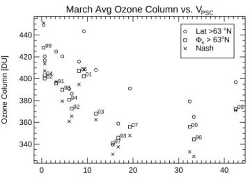
March Avg Ozone Column vs. VPSC
0 10 20 30 40
VPSC (10 6
km3
; ECMWF Analysis, 15Dec−31Mar, 400−550K) 340 360 380 400 420 440
Ozone Column [DU]
91 92 93 94 96 97 98 99 00 01 02 03 04 05 06 07 Lat >63 o N Φe > 63 o N Nash
Fig. 8. The relation between VPSCand the total column ozone in
March averaged over the Arctic polar region. Circles show averages poleward of 63◦N, squares averages poleward of 63◦N equivalent latitude, and crosses averages poleward of the vortex edge defined by the maximum gradient in potential vorticity.
3.3 Relation between the mean polar ozone column and meteorological conditions
In the Arctic, chemical ozone loss is closely related to the particular meteorological conditions in each year. Rex et al. (2004) reported that Arctic chemical loss is linearly related to a measure of the potential of polar stratospheric cloud occur-rence referred to as VPSC. VPSCis defined as the volume of
stratospheric air below the threshold temperature for the ex-istence of nitric acid trihydrate, averaged over a certain time period and altitude range (Rex et al., 2004).
VPSCis an absolute measure and is therefore strictly
com-parable only with absolute measures of ozone loss like the ozone mass deficit (e.g., Huck et al., 2007). Vortex mean ozone loss should be related to the fraction of the vortex that is activated. This effect becomes particularly important if Arctic and Antarctic conditions are compared, where the vortices have rather differnt sizes. Therefore, Tilmes et al. (2006) extended the concept of VPSC introducing the PSC
formation potential of the polar vortex (PFP),2 a measure that takes into account the size of the vortex. Here we inves-tigate whether the simple measures of polar ozone loss dis-cussed above show any relation to the measures of chlorine activation in the vortex such as VPSCand PFP.
Figure 8 shows a scatterplot of VPSCagainst column ozone
averaged over the area poleward of geometric or equiva-lent latitude 63◦N and within the vortex. Obviously, in
2PFP is calculated in the following way. For all days when a
vortex exists and for a defined altitude range, VPSC is divided by
the volume of the polar vortex, and these values are then integrated over a defined time period. Finally, this value is divided by the total number of days in the period (Tilmes et al., 2006).
March Min of Daily Avg Ozone Column vs. VPSC
0 10 20 30 40
VPSC (10 6
km3
; ECMWF Analysis, 15Dec−31Mar, 400−550K) 300 320 340 360 380 400 420 440
Ozone Column [DU]
91 92 93 94 96 97 98 99 00 01 02 03 04 05 06 07 Lat >63 o N Φe > 63 o N Nash
Fig. 9. The relation between VPSC and the minimum of March
daily average polar column ozone (symbols as in Fig. 8). The dot-ted line shows an empirical fit through the minimum ozone values for averages poleward of an equivalent latitude of 63◦N with the exception of the years 1999, 2001, and 2006 for which the final warming occurred before March (WMO, 2007); Santee, 20081. Not shown (and excluded from the fit) is the year 1995 because of poor data quality; only 3% of the data points poleward of 63◦ equiva-lent latitude are valid. The polynomial describing the fit is given by M=388.6−6.10 · V +0.178 · V2−0.00176 · V3, where V is VPSC
in 106km3 and M is the minimum of March daily average polar column ozone in Dobson units (this relation being valid for VPSC
<42.5).
contrast to the compact relation between VPSC and
chemi-cal ozone loss (Rex et al., 2004; Tilmes et al., 2004), there is no close relation between VPSCand March average ozone.
This holds irrespective of the horizontal boundary specified as the limit for the averaging. Apparently, the March aver-age ozone is a measure that does not adequately differenti-ate between chemical loss and dynamical resupply of ozone that both change substantially from year to year. Further-more, the March average ozone poleward of geometric lati-tude of 63◦N is particularly sensitive to the strong year-to-year variability in the lifetime and shape of the Arctic vortex (Waugh and Randel, 1999; Karpetchko et al., 2005). We ar-gued above that the minimum of March daily average polar column ozone should be a quantity more closely related to chemical ozone loss than those shown in Fig. 8. However, no clearly compact and especially no linear relation of the minimum of March daily column ozone with VPSCemerges.
Some outliers, e.g. the years 1999, 2001, and 2006, can be understood. For these years, the final warming was very early so that no vortex existed during March (WMO, 2007); San-tee 20081, with the consequence of a larger ozone column caused by the influx of mid-latitude ozone-rich air. Con-centrating on data for the years when the polar vortex in March was intact, we find a tighter relation between VPSC
of 8e=63◦that is indicated by the dotted line in Fig. 9. From
the three different quantities shown, the polynomial fit with this quantity has the lowest deviation (1σ =5.5 DU) from the observations and shows a (nearly) monotonic decrease with increasing VPSC.
Obviously, the minimum ozone column in the three cold-est winters (1996, 2000, and 2005) is not much lower than the minimum in moderately cold winters such as 1993 or 2003. This effect is mostly responsible for the nonlinear relation between VPSCand the minimum of March column ozone.
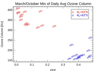
When PSC occurrence or the potential for chlorine acti-vation is compared for the Arctic and Antarctic, VPSC is no
longer a suitable measure, because the polar vortex is much larger in the Antarctic than in the Arctic; for such a compar-ison, the PFP should be used instead of VPSC (Tilmes et al.,
2006). In Fig. 10, the PFP is plotted against the minimum of daily average polar column ozone in spring, where only data points for averages poleward of 63◦equivalent latitude
are shown. The well-known fact that winter/spring temper-atures are lower in the Antarctic than in the Arctic (leading to a greater PFP, Tilmes et al., 2006) and that polar column ozone in greater in the Arctic than in the Antarctic (Dobson, 1968; WMO, 2007) is reflected in this plot. However, for this combination of meteorological and ozone measures, again no clearly compact relation emerges.
3.4 Relation between polar column ozone and chemical ozone loss
To diagnose chemical ozone destruction in the polar vortices, several methods have been developed that bring in informa-tion beyond ozone measurements which allows the impact of transport and chemistry on ozone to be disentangled (Harris et al., 2002; WMO, 2007). Here (Fig. 11), we compare chem-ical ozone loss between 380–550 K potential temperature in March deduced for the Arctic winters 1992–2005 based on the vortex average method (Chipperfield et al., 2005; Rex et al., 2006) with the two most commonly used simple mea-sures based on total ozone, namely the average polar ozone poleward of geometric latitude 63◦N in March and the min-imum of all total ozone measurements in March poleward of geometric latitude 60◦N (e.g., Newman et al., 1997; Austin et al., 2003; WMO, 2007). We also performed a similar com-parison (not shown) using chemical ozone loss deduced for the Arctic winters 1992–2003 by applying the ozone-tracer correlation method (Tilmes et al., 2004) and obtained very similar results. Clearly, there is some relation between these measures and chemical ozone loss. The stronger the chem-ical ozone loss, the lower both the average March and the minimum March total ozone are (Fig. 11, top and middle panel). However, in these two cases, the correlation is not very strong and in both cases outliers are noticeable. Fur-ther, the stronger the link between chemical ozone loss and a simple measure, the closer should the slope m of the linear fit approach minus one (this would be the value for a
year-March/October Min of Daily Avg Ozone Column
0.0 0.1 0.2 0.3 0.4 PFP 150 200 250 300 350 400
Ozone Column [DU]
92 93 94 96 97 98 99 00 01 02 03 04 05 06 92 93 94 95 96 97 98 99 00 01 02 03 04 05 Φe>63 o N Φe>63 o S
Fig. 10. The relation between PFP and the minimum of daily av-erage polar column ozone in spring for both the Arctic (March, red symbols) and the Antarctic (October, blue symbols). Only data points for averages poleward of 63◦ equivalent latitude are shown. PFP values are calculated on the basis of MetO analy-sis (Swinbank and O’Neill, 1994), averaged over the altitude re-gion 400–550 K for the period 15 December to 31 March and 15 June to 30 September for the Arctic and Antarctic, respec-tively. Note that the PFP values shown here are slightly im-proved compared to those reported by Tilmes et al. (2006), see also electronical supplement (http://www.atmos-chem-phys.net/8/ 251/2008/acp-8-251-2008-supplement.zip).
to-year variability in total ozone that is solely due to chem-ical loss). The slope calculated for the average polar ozone in March (top panel in Fig. 11) is m= − 0.25 and for the minimum column ozone (middle panel) m= − 0.14. For the minimum of daily average ozone poleward of equivalent lat-itude 63◦N (bottom panel) the strongest slope is obtained,
m= −0.53. Further, for this measure, the most compact re-lation and the best correre-lation emerges. That means, of all the simple measures considered, the new measure suggested here (Sect. 3.2.3) shows the closest correlation with chemical ozone loss.
4 Discussion
Among the quantities describing stratospheric ozone, total column ozone is the one most easily measured. Indeed, the longest atmospheric time series exist for total ozone (e.g., Dobson, 1968; Br¨onnimann et al., 2003). Long time series are a prerequisite for deriving correlation properties of total ozone and for a reliable trend analysis (e.g., Staehelin et al., 1998; Kiss et al., 2007; Vyushin et al., 2007; WMO, 2007). Moreover, the Antarctic ozone hole was discovered, and the discovery corroborated, through measurements of total col-umn ozone (Chubachi, 1984; Farman et al., 1985; Stolarski et al., 1986). However, variations in total ozone are caused
340 360 380 400 420 440
Ozone Column [DU]
avg O3 in March, lat>63 o N 92 93 94 95 96 97 98 99 00 03 05 r=−0.31 200 210 220 230 240 250 260
Ozone Column [DU]
min of all O3 obs in March, lat>60 o N 92 93 94 95 96 97 98 99 00 03 05 r=−0.26 20 40 60 80 100 120 Ozone Loss [DU] from Rex et al. 320
340 360 380 400
Ozone Column [DU]
min of daily avg O3 in March, Φe>63 o N 92 93 94 95 96 97 98 99 00 03 05 r=−0.75
Fig. 11. The relation between the observed chemical ozone loss in the Arctic (Chipperfield et al., 2005; Rex et al., 2006) and simple measures based on total ozone; compared are the two most com-monly used measures (top and middle panel) and the measure (see section 3.2.3) recommended here (bottom panel). Top panel shows the average polar ozone poleward of geometric latitude 63◦N in March, middle panel the minimum of all total ozone measurements in March poleward of geometric latitude 60◦N and bottom panel the minimum of daily average ozone poleward of equivalent latitude 63◦N. Correlation coefficients from the linear fits (r) are shown in all panels. No ozone loss values are reported for 2001 and 2006. In all fits, 1999 was excluded as the vortex broke up before March in this year.
by both chemical change and by transport, and the different impacts of these processes are often difficult to disentangle.
Transport contributions to polar ozone variability are closely controlled by the strength of the middle atmospheric (Brewer-Dobson) circulation that is driven by tropospheric wave forcing. For both the Arctic and Antarctic, a stronger-than-average planetary wave forcing in winter leads to more transport of ozone to high latitudes because of a stronger cir-culation and a higher-than-average polar lower stratospheric temperature and a weaker vortex in early spring, whereas a weaker wave forcing leads to less transport, lower polar tem-peratures in spring and to a stronger vortex (Fusco and Salby, 1999; Newman et al., 2001; Weber et al., 2003). The vari-ability in polar ozone due to the varivari-ability in wave forcing is
Min of Daily Avg Ozone Column, Φe>63 o 320 340 360 380 400 420
Ozone Column [DU]
March, Arctic 1980 1985 1990 1995 2000 2005 160 180 200 220 240 260 280
Ozone Column [DU]
October, Antarctic
Fig. 12. Time series of minimum of daily average column ozone poleward of 63◦equivalent latitude for March in the Arctic (top panel) and October in the Antarctic (bottom panel). Winters in which the vortex broke up before March (1987, 1999, 2001, and 2006) are not shown for the Arctic time series.
much larger in the Arctic than in the Antarctic, while chemi-cal loss is more persistent in Antarctica.
Here we argue that measures of chemical ozone loss based on monthly averages of total column ozone over the polar cap, although they contain information about chemical ozone loss, must be interpreted with caution. The particular value of such measures will depend on the selected definition of the equatorward boundary of the region over which averages are calculated. In the Arctic, the year-to-year variability of the size of the polar vortex has a particularly strong impact. Fur-ther, there are winters when the Artic vortex breaks up early (e.g., WMO, 2007), a fact that is often neglected in the in-terpretation of monthly mean total column ozone time series. Moreover, averages over the polar cap neither show compact relationships with meteorological measures of the extent of chlorine activation (and thus the potential for ozone destruc-tion) in the polar vortices such as VPSCand PFP nor a good
correlation with observed chemical ozone loss. Although fre-quently employed, the minimum value of daily total column ozone minima over the polar region is a particularly prob-lematic measure, insofar as it relies on a single measurement or on a single model grid point. We have shown here that for the Arctic, both in a CCM and in observations, a signifi-cant fraction of the minimum values of daily total ozone min-ima occur outside the polar vortex. Clearly, if the minimum ozone value on a particular day occurs outside the vortex, it does not provide information on halogen-driven chemi-cal ozone loss initiated by heterogeneous chlorine activation. Because of the strong chemical ozone loss in the Antarctic, this problem is much less pronounced there. It should, how-ever, become increasingly relevant for simulations of future ozone loss, when much less chemical ozone loss is expected. Based on this analysis, we must question the applicability of
a simple measure such as a minimum polar cap ozone value for both the E39/C model and observations, and strongly caution against application of this simple measure to results from other CCM simulations. It is remarkable that there is substantial variation in the magnitude of minimum total col-umn ozone in the Arctic in current model simulations ranging roughly from 220 to 320 DU whereas the observations lie in the range of 290 DU to below 200 DU (WMO, 2007, Fig. 6– 13).
Clearly, employing sophisticated measures of polar chem-ical ozone loss that show a compact correlation with mete-orological measures of chlorine activation (Rex et al., 2004; Tilmes et al., 2006) is the best method to assess the tempo-ral evolution of polar ozone loss in both models and obser-vations. However, when only total column ozone data are available, we propose that the minimum of March (or Octo-ber) daily average total ozone in the vortex (where the vor-tex boundary can be determined by the maximum gradient in PV or by an equivalent latitude criterion) should be consid-ered. This quantity is not strongly influenced by low column ozone outside the vortex and does not rely on a single mea-surement or model grid point. Further, in contrast to monthly averages, its year-to-year variability is not substantially af-fected by varying dates of vortex breakdown in the Arctic. If equivalent latitude 63◦is applied as the criterion for polar air, then the minimum of daily average total ozone in spring also shows a resonable correlation with observed chemical ozone loss (Fig. 11).
In Fig. 12, a time series is shown of the spring minimum of daily average total ozone poleward of 63◦equivalent
lat-itude for March in the Arctic and October in the Antarctic. Compared to the frequently shown figure of the temporal de-velopment of the monthly mean total ozone poleward of 63◦ geographic latitude (WMO, 2007, Fig. 4–7), Fig. 12 shows a different picture, with a stronger contrast for the Arctic. However, in both cases, the time series of minimum daily average column ozone avoids the impression of an apparent “recovery” of polar ozone since the late nineties conveyed by the customary monthly mean total ozone figure.
5 Conclusions
Quantities deduced from measurements of total column ozone are frequently used as measures of polar ozone loss. One of the most common measures is monthly mean column ozone poleward of 63◦for March and October in the Arctic
and Antarctic, respectively (WMO, 2007). For the Arctic, a latitude of 63◦is a reasonable boundary for polar air, except for winters when the vortex breaks up early. In contrast, for the Antarctic, the values of the October means (but not their year-to-year variability) are sensitive to the exact choice of 63◦. A better definition of the polar vortex boundary can be obtained using the gradient in PV (Nash et al., 1996) or equivalent latitude.
The spring minimum of daily total ozone minima pole-ward of a given latitude is a further measure that is often employed, in particular, when comparing polar ozone loss in observations and models. This is a problematic measure, in-sofar as it relies on one single measurement or on one single model grid point; for Arctic conditions, it is not unlikely that this minimum value occurs in air outside the polar vortex. We suggest that this concept should no longer be used as a measure of polar ozone loss.
Neither for the monthly mean column ozone poleward of 63◦for March and October nor for the spring minimum of daily total ozone minima can a close relation be obtained with meteorological quantities that describe the potential for polar heterogeneous chlorine activation. Likewise, neither of the two measures shows a good correlation with chemi-cal ozone loss in the vortex deduced from observations (Rex et al., 2006; Tilmes et al., 2004).
Considering the minimum of daily average total ozone poleward of 63◦ equivalent latitude (or in the vortex) in spring, avoids the problem of relying on one single data point and reduces the impact of year-to-year variability in the Arc-tic vortex break-up on ozone loss measures (see Sect. 3.2.3). This measure also shows a reasonable correlation (r=−0.75) with observed chemical ozone loss.
We propose the minimum of daily average total ozone poleward of 63◦equivalent latitude as a candidate for a
use-ful simple measure of polar ozone loss, when winters with an early vortex break-up (before March in the Arctic) are excluded. In any event, it is always preferable to employ more sophisticated measures of chemical polar ozone loss (e.g., Harris et al., 2002; Rex et al., 2004; Tilmes et al., 2006; Lemmen et al., 2006b; WMO, 2007) that bring in additional information to disentangle the impact of transport and chem-ical change on ozone.
Acknowledgements. We are grateful to S. Tilmes for helpful discussions on the manuscript and for providing the values for PFP used here. This version of the paper has been substantially improved compared to the original (ACPD) version by changes made in response to very helpful comments by an anonymous referee and by the editor G. Vaughan. We thank J. Carter-Sigglow for a stylistic and grammatical revision of the manuscript. C. L. was partly supported by the Dutch Environmental Assessment Agency (Milieu- en Natuurplanbureau Bilthoven, The Netherlands). We thank the European Centre for Medium-Range Weather Forecasts and the UK Meteorological Office for providing meteorological analyses.
Edited by: G. Vaughan
References
Austin, J., Shindell, D., Beagley, S. R., Br¨uhl, C., Dameris, M., Manzini, E., Nagashima, T., Newman, P., Pawson, S., Pitari, G., Rozanov, E., Schnadt, C., and Shepherd, T. G.: Uncertainties and assessments of chemistry-climate models of the stratosphere,
Atmos. Chem. Phys., 3, 1–27, 2003, http://www.atmos-chem-phys.net/3/1/2003/.
Balis, D., Lambert, J.-C., Roozendael, M. V., Spurr, R., Loyola, D., Livschitz, Y., Valks, P., Amiridis, V., Gerard, P., Granville, J., and Zehner, C.: Ten years of GOME/ERS2 total ozone data – The new GOME data processor (GDP) version 4: 2. Ground-based validation and comparisons with TOMS V7/V8, J. Geo-phys. Res., 112, D07307, doi:10.1029/2005JD006376, 2007. Bodeker, G. E., Scott, J. C., Kreher, K., and McKenzie, R. L.:
Global ozone trends in potential vorticity coordinates using TOMS and GOME intercompared against the Dobson network: 1978–1998, J. Geophys. Res., 106, 23 029–23 042, 2001. Bodeker, G. E., Struthers, H., and Connor, B. J.: Dynamical
con-tainment of Antarctic ozone depletion, Geophys. Res. Lett., 29, 1098, doi:10.1029/2001GL014206, 2002.
Bodeker, G. E., Shiona, H., and Eskes, H.: Indicators of Antarctic ozone depletion, Atmos. Chem. Phys., 5, 2603–2615, 2005, http://www.atmos-chem-phys.net/5/2603/2005/.
Br¨onnimann, S. and Hood, L. L.: Frequency of low-ozone events over northwestern Europe in 1952–1963 and 1990–2000, Geo-phys. Res. Lett., 30, 2118, doi:10.1029/2003GL018431, 2003. Br¨onnimann, S., Staehelin, J., Farmer, S. F. G., Svendby, T., and
Svenøe, T.: Total ozone observations prior to the IGY. I: A his-tory, Q. J. Roy. Meteor. Soc., 129, 2797–2817, 2003.
Brunner, D., Staehelin, J., K¨unsch, H.-R., and Bodeker, G. E.: A Kalman filter reconstruction of the vertical ozone distribu-tion in an equivalent latitude-potential temperature framework from TOMS/GOME/SBUV total ozone observations, J. Geo-phys. Res., 111, D12308, doi:10.1029/2005JD006279, 2006. Butchart, N. and Remsberg, E. E.: The area of the stratospheric
polar vortex as a diagnostic for tracer transport on an isentropic surface, J. Atmos. Sci., 43, 1319–1339, 1986.
Chipperfield, M. P., Feng, W., and Rex, M.: Arctic ozone loss and climate sensitivity: Updated three-dimensional model study, Geophys. Res. Lett., 32, L11813, doi:10.1029/2005GL022674, 2005.
Christensen, T., Knudsen, B. M., Streibel, M., Anderson, S. B., Be-nesova, A., Braathen, G., Davies, J., De Backer, H., Dier, H., Dorokhov, V., Gerding, M., Gil, M., Henchoz, B., Kelder, H., Kivi, R., Kyr¨o, E., Litynska, Moore, D., Peters, G., Skrivankova, P., St¨ubi, R., Turunen, T., Vaughan, G., Viatte, P., Vik, A. F., von der Gathen, P., and Zaitcev, I.: Vortex-averaged Arctic ozone depletion in the winter 2002/2003, Atmos. Chem. Phys., 5, 131– 138, 2005,
http://www.atmos-chem-phys.net/5/131/2005/.
Chubachi, S.: Preliminary result of ozone observations at Syowa station from February 1982 to January 1983, Mem. Natl. Inst. Polar Res. Spec. Issue, 34, 13–19, 1984.
Dameris, M., Grewe, V., Ponater, M., Deckert, R., Eyring, V., Mager, F., Matthes, S., Schnadt, C., Stenke, A., Steil, B., Br¨uhl, C., and Giorgetta, M. A.: Long-term changes and variability in a transient simulation with a chemistry-climate model employing realistic forcing, Atmos. Chem. Phys., 5, 2121–2145, 2005, http://www.atmos-chem-phys.net/5/2121/2005/.
Dobson, G. M. B.: Forty years’ research on atmospheric ozone at Oxford: A history, Appl. Opt., 7, 387–405, 1968.
Eyring, V., Butchart, N., Waugh, D. W., Akiyoshi, H., Austin, J., Bekki, S., Bodeker, G. E., Boville, B. A., Br¨uhl, C., Chipper-field, M. P., Cordero, E., Dameris, M., Deushi, M., Fioletov,
V. E., Frith, S. M., Garcia, R. R., Gettelman, A., Giorgetta, M. A., Grewe, V., Jourdain, L., Kinnison, D. E., Mancini, E., Manzini, E., Marchand, M., Marsh, D. R., Nagashima, T., Nielsen, E., Newman, P. A., Pawson, S., Pitari, G., Plummer, D. A., Rozanov, E., Schraner, M., Shepherd, T. G., Shibata, K., Stolarski, R. S., Struthers, H., Tian, W., and Yoshiki, M.: Assessment of tem-perature, trace species and ozone in chemistry-climate simula-tions of the recent past, J. Geophys. Res., 111, D22308, doi: 10.1029/2006JD007327, 2006.
Eyring, V., Waugh, D. W., Bodeker, G. E., Cordero, E., Akiyoshi, H., Austin, J., Beagley, S. R., Boville, B. A., Braesicke, P., Br¨uhl, C., Butchart, N., Chipperfield, M. P., Dameris, M., Deckert, R., Deushi, M., Frith, S. M., Garcia, R. R., Gettelman, A., Giorgetta, M. A., Kinnison, D. E., Mancini, E., Manzini, E., Marsh, D. R., Matthes, S., Nagashima, T., Newman, P. A., Nielsen, J. E., Paw-son, S., Pitari, G., Plummer, D. A., Rozanov, E., Schraner, M., Scinocca, J. F., Semeniuk, K., Shepherd, T. G., Shibata, K., Steil, B., Stolarski, R. S., Tian, W., and Yoshiki, M.: Multimodel pro-jections of stratospheric ozone in the 21st century, J. Geophys. Res., 112, D16303, doi:10.1029/2006JD008332, 2007.
Farman, J. C., Gardiner, B. G., and Shanklin, J. D.: Large losses of total ozone in Antarctica reveal seasonal ClOx/NOxinteraction,
Nature, 315, 207–210, 1985.
Fusco, A. C. and Salby, M. L.: Interannual variations of total ozone and their relationship to variations of planetary wave activity, J. Climate, 12, 1619–1629, 1999.
Goutail, F., Pommereau, J.-P., Lef`evre, F., Roozendael, M. V., An-dersen, S. B., K˚astad-Høiskar, B.-A., Dorokhov, V., Kyr¨o, E., Chipperfield, M. P., and Feng, W.: Early unusual ozone loss dur-ing the Arctic winter 2002/2003 compared to other winters, At-mos. Chem. Phys., 5, 665–677, 2005,
http://www.atmos-chem-phys.net/5/665/2005/.
Greenblatt, J. B., Jost, H.-J., Loewenstein, M., Podolske, J. R., Bui, T. P., Hurst, D. F., Elkins, J. W., Herman, R. L., Webster, C. R., Schauffler, S. M., Atlas, E. L., Newman, P. A., Lait, L. L., M¨uller, M., Engel, A., and Schmidt, U.: Defining the polar vortex edge from an N2O:potential temperature correlation, J. Geophys. Res.,
107, 8268, doi:10.1029/2001JD000575, 2002.
Harris, N. R. P., Rex, M., Goutail, F., Knudsen, B. M., Manney, G. L., M¨uller, R., and von der Gathen, P.: Comparison of empir-ically derived ozone loss rates in the Arctic vortex, J. Geophys. Res., 107, 8264, doi:10.1029/2001JD000482, 2002.
Hein, R., Dameris, M., Schnadt, C., Land, C., Grewe, V., K¨ohler, I., Ponater, M., Sausen, R., Steil, B., Landgraf, J., and Br¨uhl, C.: Results of an interactively coupled atmospheric chemistry-general circulation model: Comparison with observations, Ann. Geophys., 19, 435–457, 2001,
http://www.ann-geophys.net/19/435/2001/.
Hood, L. L., Soukharev, B. E., Fromm, M., and McCormack, J. P.: Origin of extreme ozone minima at middle to high northern lati-tudes, J. Geophys. Res., 106, 20 925–20 940, 2001.
Huck, P. E., Tilmes, S., Bodeker, G. E., Randel, W. J., McDonald, A. J., and Nakajima, H.: An improved measure of ozone deple-tion in the Antarctic stratosphere, J. Geophys. Res., 112, D1110, doi:10.1029/2006JD007860, 2007.
IPCC/TEAP: Special Report on Safeguarding the Ozone Layer and the Global Climate System: Issues Related to Hydrofluorocar-bons and PerfluorocarHydrofluorocar-bons, Cambridge University Press, Cam-bridge, United Kingdom, and New York, NY, USA, edited by
Metz, B., Kuijpers, L., Solomon, S., Andersen, S. O., Davidson, O., Pons, J., de Jager, D., Kestin, T., Manning, M., and Meyer, L., p. 478, 2005.
James, P. M., Peters, D., and Waugh, D. W.: Very low ozone episodes due to polar vortex displacement, Tellus, 52B, 1123– 1137, 2000.
Jin, J. J., Semeniuk, K., Manney, G. L., Jonsson, A. I., Bea-gley, S. R., McConnell, J. C., Dufour, G., Nassar, R., Boone, C. D., Walker, K. A., Bernath, P. F., and Rinsland, C. P.: Se-vere Arctic ozone loss in the winter 2004/2005: observations from ACE-FTS, Geophys. Res. Lett., 33, L15801, doi:10.1029/ 2006GL026752, 2006.
Jones, A. E. and Shanklin, J. D.: Continued decline of total ozone over Halley, Antarctica since 1985, Nature, 376, 409–411, 1995. Karpetchko, A., Kyr¨o, E., and Knudsen, B. M.: Arctic and Antarctic polar vortices 1957-2002 as seen from the ERA-40 reanalyses, J. Geophys. Res., 110, D21109, doi:10.1029/2005JD006113, 2005.
Keil, M., Jackson, D. R., and Hort, M. C.: The January 2006 low ozone event over the UK, Atmos. Chem. Phys., 7, 961–972, 2007,
http://www.atmos-chem-phys.net/7/961/2007/.
Kiss, P., M¨uller, R., and J´anosi, I. M.: Long-range correlations of extrapolar total ozone are determined by the global atmospheric circulation, Nonlin. Processes Geophys., 14, 435–442, 2007, http://www.nonlin-processes-geophys.net/14/435/2007/. Knudsen, B. M.: Interactive comment on “Uncertainties and
as-sessments of chemistry-climate models of the stratosphere” by Austin, J., Shindell, D., Beagley, S. R., Bruehl, C., Dameris, M., Manzini, E., Nagashima, T., Newman, P., Pawson, S., Pitari, G., Rozanov, E., Schnadt, C., and Shepherd, T. G., Atmos. Chem. Phys. Discuss., 2, S323–S324, 2002.
Kr¨uger, K., Naujokat, B., and Labitzke, K.: The unusual midwinter warming in the southern hemisphere stratosphere 2002: A com-parison to northern hemisphere phenomena, J. Atmos. Sci., 62, 603–613, 2005.
Lary, D. J., Chipperfield, M. P., Pyle, J. A., Norton, W. A., and Riishøjgaard, L. P.: Three-dimensional tracer initialization and general diagnostics using equivalent PV latitude-potential-temperature coordinates, Q. J. Roy. Meteor. Soc., 121, 187–210, 1995.
Lemmen, C.: Future polar ozone: predictions of Arctic ozone re-covery in a changing climate, Ph D thesis, Bergische Universit¨at Wuppertal, 2005.
Lemmen, C., Dameris, M., M¨uller, R., and Riese, M.: Chemical ozone loss in a chemistry-climate model from 1960 to 1999, Geophys. Res. Lett., 33, L15820, doi:10.1029/2006GL026939, 2006a.
Lemmen, C., M¨uller, R., Konopka, P., and Dameris, M.: Critique of the tracer-tracer correlation technique and its potential to analyse polar ozone loss in chemistry-climate models, J. Geophys. Res., 111, D18307, doi:10.1029/2006JD007298, 2006b.
Manney, G. L., Froidevaux, L., Waters, J. W., Zurek, R. W., Read, W. G., Elson, L. S., Kumer, J. B., Mergenthaler, J. L., Roche, A. E., O’Neill, A., Harwood, R. S., MacKenzie, I., and Swin-bank, R.: Chemical depletion of ozone in the Arctic lower strato-sphere during winter 1992–1993, Nature, 370, 429–434, 1994. Manney, G. L., Froidevaux, L., Santee, M. L., Zurek, R. W., and
Waters, J. W.: MLS observations of Arctic ozone loss in 1996-97,
Geophys. Res. Lett., 24, 2697–2700, doi:10.1029/97GL52827, 1997.
Manney, G. L., Froidevaux, L., Santee, M. L., Livesey, N. J., Sabutis, J. L., and Waters, J. W.: Variability of ozone loss during Arctic winter (1991 to 2000) estimated from UARS Microwave Limb Sounder measurements, J. Geophys. Res., 108, 4149, doi: 10.1029/2002JD002634, 2003.
Manney, G. L., Santee, M. L., Froidevaux, L., Hoppel, K., Livesey, N. J., and Waters, J. W.: EOS MLS observations of ozone loss in the 2004-2005 Arctic winter, Geophys. Res. Lett., 33, L04802, doi:10.1029/2005GL024494, 2006.
McKenna, D. S., Jones, R. L., Austin, J., Browell, E. V., Mc-Cormick, M. P., Krueger, A. J., and Tuck, A. F.: Diagnostic studies of the Antarctic vortex during the 1987 Airborne Antarc-tic Ozone Experiment: Ozone miniholes, J. Geophys. Res., 94, 11 641–11 668, 1989.
McKenna, D. S., Grooß, J.-U., G¨unther, G., Konopka, P., M¨uller, R., Carver, G., and Sasano, Y.: A new Chemical Lagrangian Model of the Stratosphere (CLaMS): 2. Formulation of chem-istry scheme and initialization, J. Geophys. Res., 107, 4256, doi: 10.1029/2000JD000113, 2002.
M¨uller, R.: Impact of cosmic rays on stratospheric chlorine chemistry and ozone depletion, Phys. Rev. Lett., 91, 058502, doi:10.1103/PhysRevLett.91.058502, 2003.
M¨uller, R. and G¨unther, G.: A generalized form of Lait’s modified potential vorticity, J. Atmos. Sci., 60, 2229–2237, 2003. M¨uller, R., Crutzen, P. J., Grooß, J.-U., Br¨uhl, C., Russel III, J. M.,
and Tuck, A. F.: Chlorine activation and ozone depletion in the Arctic vortex: Observations by the Halogen Occultation Exper-iment on the Upper Atmosphere Research Satellite, J. Geophys. Res., 101, 12 531–12 554, 1996.
M¨uller, R., Tilmes, S., Konopka, P., Grooß, J.-U., and Jost, H.-J.: Impact of mixing and chemical change on ozone-tracer relations in the polar vortex, Atmos. Chem. Phys., 5, 3139–3151, 2005, http://www.atmos-chem-phys.net/5/3139/2005/.
Nash, E. R., Newman, P. A., Rosenfield, J. E., and Schoeberl, M. R.: An objective determination of the polar vortex using Ertel’s po-tential vorticity, J. Geophys. Res., 101, 9471–9478, 1996. Newman, P. A. and Nash, E. R.: The unusual southern hemisphere
stratosphere winter of 2002, J. Atmos. Sci., 62, 614–628, 2006. Newman, P. A., Gleason, F., McPeters, R., and Stolarski, R.:
Anomalously low ozone over the Arctic, Geophys. Res. Lett., 24, 2689–2692, doi:10.1029/97GL52381, 1997.
Newman, P. A., Nash, E. R., and Rosenfield, J. E.: What con-trols the temperature of the Arctic stratosphere during the spring?, J. Geophys. Res., 106(D17), 19 999–20 010, doi:10. 1029/2000JD000061, 2001.
Newman, P. A., Kawa, S. R., and Nash, E. R.: On the size of the Antarctic ozone hole, Geophys. Res. Lett., 31, L21104, doi:10. 1029/2004GL020596, 2004.
Petzoldt, K., Naujokat, B., and Neugebohren, K.: Correlation be-tween stratospheric temperature, total ozone and tropospheric weather systems, Geophys. Res. Lett., 21, 1203–1206, doi: 10.1029/93GL03020, 1994.
Proffitt, M. H., Margitan, J. J., Kelly, K. K., Loewenstein, M., Podolske, J. R., and Chan, K. R.: Ozone loss in the Arctic polar vortex inferred from high altitude aircraft measurements, Nature, 347, 31–36, 1990.
of ozone minima at northern midlatitudes, J. Geophys. Res., 105, 12 169–12 180, 2000.
Rex, M., Salawitch, R. J., Harris, N. R. P., von der Gathen, P., Schulz, G. O. B. A., Deckelman, H., Chipperfield, M., Sinnhu-ber, B.-M., Reimer, E., Alfier, R., Bevilacqua, R., Hoppel, K., Fromm, M., Lumpe, J., K¨ullmann, H., Kleinb¨ohl, A., von K¨onig, H. B. M., K¨unzi, K., Toohey, D., V¨omel, H., Richard, E., Aiken, K., Jost, H., Greenblatt, J. B., Loewenstein, M., Podolske, J. R., Webster, C. R., Flesch, G. J., Scott, D. C., Herman, R. L., Elkins, J. W., Ray, E. A., Moore, F. L., Hurst, D. F., Romanshkin, P., Toon, G. C., Sen, B., Margitan, J. J., Wennberg, P., Neuber, R., Allart, M., Bojkov, B. R., Claude, H., Davies, J., Davies, W., De Backer, H., Dier, H., Dorokhov, V., Fast, H., Kondo, Y., Kyr¨o, E., Litynska, Z., Mikkelsen, I. S., Molyneux, M. J., Moran, E., Nagai, T., Nakane, H., Parrondo, C., Ravegnani, F., Viatte, P. S. P., and Yushkov, V.: Chemical depletion of Arctic ozone in winter 1999/2000, J. Geophys. Res., 107, 8276, doi: 10.1029/2001JD000533, 2002.
Rex, M., Salawitch, R. J., von der Gathen, P., Harris, N. R. P., Chipperfield, M. P., and Naujokat, B.: Arctic ozone loss and climate change, Geophys. Res. Lett., 31, L04116, doi:10.1029/ 2003GL018844, 2004.
Rex, M., Salawitch, R. J., Deckelmann, H., von der Gathen, P., Harris, N. R. P., Chipperfield, M. P., Naujokat, B., Reimer, E., Allaart, M., Andersen, S. B., Bevilacqua, R., Braathen, G. O., Claude, H., Davies, J., De Backer, H., Dier, H., Dorokov, V., Fast, H., Gerding, M., Godin-Beekmann, S., Hoppel, K., John-son, B., Kyr¨o, E., Litynska, Z., Moore, D., Nakane, H., Parrondo, M. C., Risley Jr., A. D., Skrivankova, P., St¨ubi, R., Viatte, P., Yushkov, V., and Zerefos, C.: Arctic winter 2005: Implications for stratospheric ozone loss and climate change, Geophys. Res. Lett., 33, L23808, doi:10.1029/2006GL026731, 2006.
Schnadt, C.: Untersuchung der zeitlichen Entwicklung der stratosph¨arischen Chemie mit einem interaktiv gekoppelten Klima-Chemie-Modell, Ph D thesis, Universit¨at M¨unchen, In-stitut f¨ur Physik der Atmosph¨are des DLR, Oberpfaffenhofen, 2001.
Schnadt, C., Dameris, M., Ponater, M., Hein, R., Grewe, V., and Steil, B.: Interaction of atmospheric chemistry and climate and its impact on stratospheric ozone, Clim. Dynam., 18, 501–517, 2002.
Shepherd, T. G.: Large-Scale Atmospheric Dynamics for Atmo-spheric Chemists, Chem. Rev., 103, 4509–4532, doi:10.1021/ cr020511z, 2003.
Staehelin, J., Kegel, R., and Harris, N. R. P.: Trend analysis of the homogenized total ozone series of Arosa (Switzerland), 1926-1996, J. Geophys. Res., 103, 5827–5841, 1998.
Stolarski, R. S., Krueger, A. J., Schoeberl, M. R., McPeters, R. D., Newman, P. A., and Alpert, J. C.: Nimbus 7 satellite measure-ments of the springtime Antarctic ozone decrease, Nature, 322, 808–811, 1986.
Swinbank, R. and O’Neill, A.: A Stratosphere-troposphere data as-similation system, Mon. Weather Rev., 122, 686–702, 1994. Tilmes, S., M¨uller, R., Grooß, J.-U., and Russell, J. M.: Ozone loss
and chlorine activation in the Arctic winters 1991–2003 derived with the tracer-tracer correlations, Atmos. Chem. Phys., 4, 2181– 2213, 2004,
http://www.atmos-chem-phys.net/4/2181/2004/.
Tilmes, S., M¨uller, R., Engel, A., Rex, M., and Russell III, J.: Chemical ozone loss in the Arctic and Antarctic stratosphere between 1992 and 2005, Geophys. Res. Lett., 33, L20812, doi: 10.1029/2006GL026925, 2006.
Tilmes, S., Kinnisen, D., M¨uller, R., Sassi, F., Marsh, D., Boville, B., and Garcia, R.: Evaluation of heterogeneous processes in the polar lower stratosphere in the Whole Atmosphere Com-munity Climate Model, J. Geophys. Res., D24301, doi:10.1029/ 2006JD008334, 2007.
von Hobe, M., Ulanovsky, A., Volk, C. M., Grooß, J.-U., Tilmes, S., Konopka, P., G¨unther, G., Werner, A., Spelten, N., Shur, G., Yushkov, V., Ravegnani, F., Schiller, C., M¨uller, R., and Stroh, F.: Severe ozone depletion in the cold Arctic winter 2004-05, Geophys. Res. Lett., 13, L17815, doi:10.1029/2006GL026945, 2006.
Vyushin, D., Fioletov, V. E., and Shepherd, T. G.: Impact of long-range correlations on trend detection in total ozone, J. Geophys. Res., 112, D14307, doi:10.1029/2006JD008168, 2007.
Waugh, D. W. and Randel, W. J.: Climatology of Arctic and Antarc-tic polar vorAntarc-tices using ellipAntarc-tical diagnosAntarc-tics, J. Atmos. Sci., 56, 1594–1613, 1999.
Weber, M., Eichmann, K.-U., Bramstedt, K., Hild, L., Richter, A., Burrows, J. P., and M¨uller, R.: The cold Arctic winter 1995/96 as observed by GOME and HALOE: Tropospheric wave activity and chemical ozone loss, Q. J. Roy. Meteor. Soc., 128, 1293– 1319, 2002.
Weber, M., Dhomse, S., Wittrock, F., Richter, A., Sinnhuber, B., and Burrows, J. P.: Dynamical control of NH and SH win-ter/spring total ozone from GOME observations in 1995–2002, Geophys. Res. Lett., 30, 1583, doi:10.1029/2002GL016799, 2003.
WMO: Scientific assessment of ozone depletion: 1998, Global Ozone Research and Monitoring Project-Report No. 44, Geneva, Switzerland, 1999.
WMO: Scientific assessment of ozone depletion: 2002, Global Ozone Research and Monitoring Project-Report No. 47, Geneva, Switzerland, 2003.
WMO: Scientific assessment of ozone depletion: 2006, Global Ozone Research and Monitoring Project-Report No. 50, Geneva, Switzerland, 2007.