HAL Id: halshs-00465709
https://halshs.archives-ouvertes.fr/halshs-00465709
Preprint submitted on 21 Mar 2010HAL is a multi-disciplinary open access archive for the deposit and dissemination of sci-entific research documents, whether they are pub-lished or not. The documents may come from
L’archive ouverte pluridisciplinaire HAL, est destinée au dépôt et à la diffusion de documents scientifiques de niveau recherche, publiés ou non, émanant des établissements d’enseignement et de
Distributed Lag Models and Economic Growth:
Evidence from Cameroon
Boniface Bounoung Fouda
To cite this version:
Boniface Bounoung Fouda. Distributed Lag Models and Economic Growth: Evidence from Cameroon. 2010. �halshs-00465709�
Distributed Lag Models and Economic Growth:
Evidence from Cameroon
January 22, 2010
Abstract
This paper studies the intertemporal effects of various economic variables on the cameroonian growth. Using a Geometric Lag Model, we nd out that 50% of the total effect of variables used is accomplished in less than half of a year. When we employ a Polynomial Distributed Lag, we nd out that even if investment has a positive impact on growth in the current year, but in the presence of government expenditures, this effect becomes negative after one year due probably to the eviction effect. In addition, we nd out that the consumption causes economic growth after three years whereas economic growth causes the consumption after only one year. The main lesson from this study is that any economic policy to sustain economic growth must boost in priority investment and foreign direct investment. The government should pursue policies that stimulate production instead to encourage consumption.
JEL classi cation: C32, C50, D40, O4
Keywords: Distributed Lag Models, Geometric Distributed Lag, Polyno-mial Distributed Lag, Economic Growth
1 Introduction
The issue of which factors affect economic growth is one of the most im-portant that economists study since several years. As evidenced by the literature estimating growth models, the wide variation in results can be partly attributed to the different theories, samples and econometric methodologies. Initially, the key issue of those studies was to explain the difference in growth performance among economies (divergence/convergence) and later, to identify the determining factors economic growth.
There are two main theories that discuss the determinants of economic growth: the neoclassical growth model1of Solow (1956) and Swan (1956) which has
em-phasised the importance of investment and more recent, the theory of endogenous growth developed by Romer (1986), Lucas (1988) and Mankiw, Romer & Weil (1992)2. This theory has drawn attention to human capital and innovation capacity.
Furthermore, important contributions on economic growth have been provided by Myrdal (1957) on cumulative causation theory3, and by Krugman (1991) and Fujita
& alii. (1999) on the New Economic Geography4. In addition, other explanations
have highlighted the signi cant role of non-economic factors on economic perfor-mance. These developments gave rise to a discussion that distinguishes between "fundamental" and "proximate" sources of growth. The former refers to the issues such as accumulation of capital, labour and technology while the latter refers to the non-economic factors. This theoritical approach suggests the signi cant role of institutions (Jutting, 2003), social-cultural factors (Knack-Keefer, 1997), polit-ical determinants (Brunetti, 1997), geography (Gallup & alii., 1999) and climatic change (Hope, 2005; Stern, 2006).
Applied studies have identi ed many other determinants of economic growth. Fry (1978, 1980) has proposed that interest rates affect growth through investment, Gupta (1987) found a positive impact of in ation on economic growth but, Lahiri (1988) and Edwards (1995) suggested that this effect depends of the countries used in the sample. Acemoglu & Ventura (2001) found that an increase in the terms of trade may encourage accumulation and growth by increasing price factor. Bal-asubramanyan & alii. (1998) and Borensztein & alii. (1998) found that even if the positive correlation between Foreign Direct Investment (FDI) and economic growth is obvious, but in the context of Less Developed Countries (LDC's), this
1The basic assumptions of their model are: constant returns to scale, diminishing marginal
pro-ductivity of capital, exogenously determined technical progress and substitutability between capital and labour. This model assumes that growth is an inexorable exogenous process.
2This theory suggests that the introduction of new accumulation factors, such as knowledge,
innovation are a signi cant source of the self-maintained economic growth.
3Essential of this theory is that initial conditions determine economic growth in a self-sustained
and incremental way.
4The central assumption of this theory is that, economic activity tends to agglomerate in a speci c
region and choose a location with a large local demand resulting in a self-reinforcing process. The New Economic Geography is mainly concerned by the location of economic activities, agglomeration and specialization rather than economic growth analysis
relation occurs only under certain conditions (pursuing export promotion policies, suf cient human capital threshold). The last most important factor of economic growth can be the ux of trade, also called openness. Frankel & Romer (1999) found that openness, measured as a ratio of export plus import to GDP, has a pos-itive impact on economic growth, but Romalis (2007) suggested that this result depends of the period used5.
Numerous of empirical studies spawned by growth theory use cross-section regressions (Sala-i-Martin, 1997) or logitudinal analysis (Nerlove, 1996). In the last case, some results have been incured by a dynamic model, specially by in-cluding as explanatory variable, the lag of dependant variable -dynamic panel data regressions- (Presbitero, 2006). Another alternative approach of empirical studies of growth uses the times series modelling. This approach has been developped by Quah (1992) and Bernard & Durlauf (1995). Most of these studies assess the rela-tionship between growth and its determinants only in the long-run process but none of them uses the distributed lag model. However, economic theory suggests that the effects of independent variables on dependent variables have a "dynamic" com-ponent. In concrete terms, these effects occur neither instantaneously nor solely in the long term but are spread, or distributed, over time.
The main contribution of this paper is to highlight the intertemporal effects of some determinants of Cameroon's economic growth because we have observed an erratic evolution of growth rate ( gure 1). Pursuing this goal, our paper is organized as follows: in section 2, we present the econometric models. Section 3 describes the data used, section 4 presents and discusses the empirical results. Finally, in section 5, we conclude.
2 Econometric Models
Assess the intertemporal effects of the explanatory variables on dependant variable must be done by using Dynamic Models. These models can be divided into three categories:
a)- models lagging both independent and dependent variables6,
b)- models lagging only dependent variable7and
c)- models lagging only independent variables8.
In this study, we will use only the last one called Distributed Lag Models (DLM). As we described above, there are three types of DLM: Geometric
Dis-5Futhermore, Tsangarides (2005) and Presbitero (2006) found a negative link between debt
(ex-ternal debt) and growth.
6It's the case of Error Correction Models. 7For exemple, Partial Adjustment Models.
8Case of Geometric Distributed Lag Models (without koyck transformation), Arithmetic
tributed Lag, Arithmetic Distributed Lag and Polynomial (Almon) Distributed Lag Models.
2.1 Arithmetic Distributed Lag Models
Algebraically, we can represent this lag effect by saying that economic out-come ytis affected by the values of a change in a variable x not only at time t but
also at time t 1, t 2; t 3 and so on. Then, we can write:
yt= z(xt; xt 1; xt 2; :::) (1)
Models like (1) describe the evolving economy and its reaction over time. The considered period depends of the length of the lag. In fact, we have in nitive dis-tributed lag models and nitive disdis-tributed lag models. The ini tive disdis-tributed lag models represented in equation (1) portrays the effects as lasting, essentially, for-ever. In the nitive distributed lag model, represented in equation (2), we assume that the effect of variable xt affects economic outcomes ytonly for a certain xed
period of time.
yt= z(xt; xt 1; xt 2; :::xt L) (2)
The general form of a distributed lag model can be written as follows:
yt = + V(B)xt+ t (3)
with V(B) = v0+ v1B1+ v2B2+ :::::: + vLBL (4)
B is the lag operator.
Equation (3) can also be written as follows:
yt= + L
X
l=0
vlxt l+ t (5)
where is the intercept, vl is a parameter called a distributed lag weight, it
mea-sures the effect of xt l on yt, all other things held constant. It's also called short
run multiplier when one period is considered. tis an uncorrelated error variable.
We assume that E( t) = 0, var( t) = 2and cov( t s) = 0. The main assumption
of arithmetic distributed lag models is that the coef cients are supposed to decline arithmetically (on a straight line).
Equation (5) can be estimated by Ordinary Least Squares (OLS) if the error term has usual desirable properties. However, collinearity is often a serious prob-lem in such models. For reducing the effects of collinearity, the Polynomial Dis-tributed Lag Models (PDLM) imposes a shape on lag distribution.
2.2 Polynomial Distributed Lag Models (PDLM)
The Polynomial Distributed Lag model also called Almon distributed lag model is a Lth-order distributed lag model with the following form:
yt= + v0xt+ v1xt 1+ v2xt 2+ v3xt 3+ ::::::: + vLxt L+ t (6)
where the impulse–response function is constrained to lie on a polynomial of de-gree p. Requiring the impulse–response function to lie on a polynomial imposes L pconstraints on the structural parameters of the model. Following Fomby & alii.(1984), it is possible to determine the form of the constraints. The rst one concerns the effect of changes in xt lon expected yt E(yt) is:
@E(yt)
@xt l
= vl= 0+ 1l + 2l2+ 3l3+ :::::: + plp with l = 0; ::::; L (7)
The futher constraint in considering equation (7) is:
p < L (8)
Substituting the constraints (equation 7) into the nite-order distributed lag model (equation 6) yields a reduced form representation:
yt= + L
X
l=0
( 0+ 1l + 2l2+ 3l3+ :::::: + plp)xt l+ t (9)
Consistent and ef cient estimates of the structural parameters, subject to the L- p constraints, can be obtained via Constrained Ordinary Least Squares (COLS). But according to Gujarati (2003), it is also possible to get consistent and ef cient estimates by using OLS if the reduced form of equation (9) is used. To obtain this reduced form, we transform equation (9) as follows:
yt= + 0T0;t+ 1T1;t+ 2T2;t+ 3T3;t+ :::::: + pTp;t+ t (10) where T0;t= L P l=0 xt l T1;t = L P l=0 lxt l T2;t= L P l=0 l2xt l T3;t= L P l=0 l3xt l :: :: Tp;t= L P lpx t l (11)
One of the important functional assumption of the PDLM is that the immediate impact might well be less than the impact after several years, quarters, or months. After reaching its maximum, the policy effect diminishes for the remainder of the nite lag. The main advantages of this model are exibility and reduction of the multicollinearity issue. We also note that imposing restrictions on parameters leads to bias unless the restrictions are true. This type of restrictions also exists in the geometric distributed lag models.
2.3 Geometric Distributed Lag Models (GDLM)
The idea of this type of model was rst introduced by Koyck (1954). This model is an in nite distributed lag model. In constrat to the equation (6), the gen-eral form of the in nite distributed lag models is:
yt= + v0xt+ v1xt 1+ v2xt 2+ v3xt 3+ :::::: + t (12)
In that model, ytis taken to be a function of xtand all its previous values. Koyck
(1954) assumes that all the coef cients (v0; v1; v2; v3; ::::; vL) have the same signe
and decline geometrically. That is
vl= v0 l; j j < 1 (13)
is the rate of decay while 1 represents the speed of adjustment. This model supposes that the most recent past weights are more heavily than the most distant past. By substituting equation (13) into equation (12), we obtain:
yt = + v0xt+ v0 1xt 1+ v0 2xt 2+ v0 3xt 3+ :::::: + t (14)
= + v0(xt+ xt 1+ 2xt 2+ 3xt 3+ :::::) + t (15)
This model has three parameters, an intercept, v0 a scale factor and which
controls the rate at which the weight's explanatory variables declines.
Koyck transformation converts equation (15) to an autoregressive model. In concrete terms, Koyck multiplies the one period lag of equation (15) by ; and substracts that result from the same equation (15) as follows:
yt yt 1= 2 4 [ + v0(xt+ xt 1+ 2xt 2+ 3xt 3+ ::) + t] [ + v0(xt 1+ xt 2+ 2xt 3 + 3xt 4+ ::) + t 1] 3 5 (16)
After rearrangement, we obtain
yt yt 1= (1 ) + v0xt+ ( t t 1) (17)
To solve yt, we obtain the Koyck form of the geometric lag;
The long-run mutiplier is:
v0(1 + + 2+ 3+ :::::::) =
v0
1 (19)
The combined effect before the end of considered period is called interim mul-tiplier. For exemple v0 + v0 2+ v0 3:As we can observe, this model has two
features: the rst is that one of the explanatory variables is the lagged dependent variable, yt 1: The second is that the error term vt depends on etand on et 1.
Consequently, yt 1 and the error term might be correlated9, since equation (17)
shows that yt 1depends directly on et 1.
Despite the solving of the multicollinearity issue or the estimation of a few parameters, this model is very restrictive. Nevertheless, in this study, we will use
Almon and Koyck models
3 Empirical Pattern and Data analysis
3.1 Empirical StrategyThe theoritical models described in section 1 give us some tools to explain
why some countries growth faster than others. By indenti ng the determining fac-tors economic growth, the empirical literature showed that the direction but also the level of impact of those determinants depend on the considered sample. For our general pattern, we can write that the output (yt) is function of its deteminants
(xt) vector of explanatory variables-:plus a random term ( t):
yt= (xt) + t (20)
Due to the fact that our purpose is to estimate the spread (year after year) of the economic policy's variables on economic growth, we will take into account mainly, the variables used in the equation of goods and services market equilib-rium. These variables are Consumption, Investment, Goverment expenditures, Exports, Imports and Gross Domestic Product. We will add merely two control variables: Foreign Direct Investment and In ation. We decided to build our model with in ation and FDI because these two variables can affect economic growth in the short run10. Levine and Renelt (1992) list over 50 possibilities amont the
range of controls appeared in the empirical literature. Following equation (3), our
9We will discuss more about it in the fourth section (how to detect this serial corelation and how
to solve it).
10This paper consciously avoids an evaluation of political factors and education because we wanted
empirical pattern can be written as follows: ln gdprt= 2 6 6 6 6 6 6 6 4 + L P l=0 v1;lln cpit l+ L P l=0 v2;lln investt l + L P l=0 v3;lln govt l+ L P l=0 v3;lln trbalt l + L P l=0 v4;lln f dit l+ L P l=0 v5;lln const l+ t 3 7 7 7 7 7 7 7 5 (21)
where gdprt is the real GDP (dollar of 2000). cpi is the consumption price
in-dex, invest is the investment, gov is the government expeditures, trbal is the trade balance, fdi is the foreign direct investment. The last variable is cons which rep-resents the consumption. t is the random disturbance term which is assumed to
follow the standard assumptions of classical linear regression model. is the in-tercept.
In fact, the speci cation used depends of the structure of distributed lag. In the case of polynomial distributed lag (PDL), the speci cation used is the same as equation (21) but with equation (7) as a constraint. As we said above, the PDL is a nite distributed lag model, for that, we must determine the maximum length of lag (L). To solve this issue, we use Akaike Information Criterion (AIC) to assess the goodness of t for lag lengths. In accordance with this criterion, we found 2 as a maximum length of lag11. To respect the constraint which suggests that the degree
of polynomial must be lesser than the number of lag (equation 7), we choose 1. Equation (7) can be rewritten as follows:
vl= 0+ 1l
with l = 0; ::::; 2
(22)
Finally, the empirical equation used in the case of PDL is as follows:
ln gdprt= 2 6 6 6 6 6 6 6 4 + 2 P l=0 ( 0+ 1l ) ln cpit l+ 2 P l=0 ( 0+ 1l ) ln investt l + L P l=0 ( 0+ 1l ) ln govt l + 2 P l=0 ( 0+ 1l ) ln trbalt l + 2 P l=0 ( 0+ 1l) ln f dit l+ 2 P l=0 ( 0+ 1l) ln const l+ t 3 7 7 7 7 7 7 7 5 (23) According to the econometric theory, consistent and ef cient estimates of the structural parameters of equation (23) can be obtained with COLS-(McDowell, 2004). An alternative approach to obtain consistent estimators of PDL is to apply rst, OLS in equation (24) which is the reduced form of equation (23). After that, it's possible to compute the estimated Almon distributed lag weights (coef cients,
standard errors, statistics tests and signi cance level) by using the delta method (Appendix B). ln gdprt= + 0T0;t+ 1T1;t+ t (24) where T0;t= 2 6 6 4 2 P l=0 ln cpit l+ 2 P l=0 ln investt l+ 2 P l=0 ln govt l + 2 P l=0 ln trbalt l+ 2 P l=0 ln f dit l+ 2 P l=0 ln const l 3 7 7 5 T1;t = 2 6 6 4 2 P l=1 l (ln cpit l) + 2 P l=1 l (ln investt l) + 2 P l=1 l (ln govt l) + 2 P l=1 l (ln trbalt l) + 2 P l=1 l (ln f dit l) + 2 P l=1 l (ln const l) 3 7 7 5 (25)
If the lags are geometrically distributed, the speci cation presented below sterns from Koyck transfomation:12
ln gdprt= (1 ) + ln gdprt 1+ v0ln xt+ t (26)
The empirical pattern of Koyck model is:
ln gdprt=
2 4
(1 ) + ln gdprt 1+ v1;0ln cpit
+v2;0ln investt+ v3;0ln govt+ v4;0ln trbalt
+v5;0ln f dit+ v6;0ln const+ t
3
5 (27)
v0is a scale factor, which controls the rate at which the weight declines, 1
is the speed of adjustment. t= ( t t 1) , it is the error term.
3.2 Data analysis
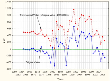
As we described above, all the variables are expressed in logarithm and are divided by the GDP except cpi (consumption price index). Due to the presence of negative values in trade balance and foreign direct investment (FDI), they have been transformed before using the logarithm function. The equation used is xT r
t =
xt+ j k j +1 with k = min xt if xt 2 [0; 1]. xt is the original variable,
xT rt is the new variable. Figures 1 and 2 show that the sequences of the change of FDI and trade balance are not modi ed. The consumption price index in base 2000 has been computed by using retropolation method13 from the data of World
Developpement Indicators. The data of the rest of variables also come from World Development Indicators for the period from 1960 to 2007.
12We will dwell upon the methods of estimation used in the next section. 13For more details, see Gómez V. & Maravall A. (1994).
4 Results and Discussion
Before running our regressions, we analyze rst the correlation between all the variables. The correlation matrix presented in appendix A shows the signi cant and high correlation between government expenditures and consumption (0,91). This result suggests that, if we run a regression with these two variables, estimators obtained will have a bias.
Another problem which arises in any economic time series analysis concerns the non-stationarity of the variables. Many empirical studies have found that key macroeconomic variables such as GDP, in ation are often non stationary. Re-gressions involving non-stationary variables may result in spurious results. Szeto (2001) notes that there are three solutions to the problem of spurious regression. The rst approach is to determine the stationarity of the variables before estimat-ing. The second approach is to add the lagged value of the dependent variable. The last method is to consider the cointegration approach. We employ the rst two approaches in this paper. Thus, in the case of Koyck model (3.1), we don't need to determine the stationarity of the variables, but before using the polynomial distrib-uted lag model, we ran the unit root tests of the variables. This has been done using the Augmented Dickey-Fuller tests (ADF), for that, we used the strategy of Dickey & Pantula (1987). We found out that: consumption, in ation and government ex-penditures are I(1) while investment, FDI, trade balance and growth rate are I(0). Moreover, Gujarati (2005) showed that the hypothesis of cointegrated variables is not crucial in the case of distributed lag models. The details of the unit root tests are presented in appendix C.
4.1 Estimates based on the Koyck transformation
The obtained results from running Koyck model are displayed in Table 1. We have ran two regressions, in the rst one (Model 1), we include consumption, in the second one (Model 2), we take off this variable and we include government expenditures. Due to the presence of lagged dependent variable such as explanatory variables, we have performed the Durbin h-test to analyze the serial correlation of the error term. The null hypothesis of no autocorrelation have been rejected in the two models suggesting that OLS can be used. We have also performed the Cook-Weisberg test, we found out that the null hypothesis of constant variance of disturbances have been accepted in Model 1 but rejected in Model 2; this latter has been regressed by using OLS with robust variance estimates.
The rst lesson from Table 1 is that the rate of decay is very small suggesting a high speed of adjustment of the effects of explanatory variables on economic growth14. This result shows that the effects of the determinants of economic growth
disappear quickly. The computation of Median Lag15shows that 50 % of the total
effect of explanatory variables is accomplished in less than half of a year. For
14The average rate of decay is 0.065 point. 15Median Lag (Med Lag)= log 2
example, concerning the variable of investment, more than 90% of the total effect of this variable disappears after the current year. In this way, the potential growth becomes certainly weak.
The second lesson from Table 1 is that all the signi cant variables have the same sign in the two models except Balance of Trade. This variable is positive in the presence of government expeditures but negative when we considered con-sumption. With this result, we can assume that in the presence of consumption, trade balance bears negatively upon economic growth, the magnitude of total ef-fect is -0.62 %16. The Model 1 of Table 1 also shows that the consumption as
a self-powered variable doesn't have a signi cant impact on economic growth17.
This latter result contributes probably to the weakness of growth effect of the pre-vious period (lagged independent variable). This effect is about 9 % in the model with government expenditures, but when we take into account consumption, this effect is shortned to 3.5%. The two models of Table 1 show that investment and consumption price index have a positive impact on economic growth, the total ef-fect (in average) of price index on growth rate is 5.8%, whereas the average total effect of investment is 12.4%. In Model 2, we observe that the effect of government expenditures is signi cant and negatively correlated with economic growth. This effect is high since an increase of 1% of the ratio of government expenditures to GDP runs down growth rate about 19.4%. In the short run analysis, we observe that an increase of 1% of the ratio of government expenditures to GDP decreases the current annual growth rate about 17.6 % . This result could lead one to conclude that the orientation of cameroonian government expenditures is not enough ef -cient18. Table 1 also shows that Foreign Direct Investment (FDI) is not signi cant
despite that its sign is always positive.
In spite of the help of Koyck model to capture the received effect of economic growth from the previous year, this model remains restrictive because it imposes that the lagged effects of explanatory variables must have the same sign as the current effect, and they must be geometrically damped as lags increase. That's why, we will present in the next sub section the results obtained by using a Polynomial Distributed Lag Model which has more exible assumptions.
4.2 Estimates using an Almon lag structure
Table 2 summarises the results of Almon polynomial coef cients from run-ning equation (10). Table 3 gives the results of Almon rst order distributed lag obtained by applying the delta method on the estimators of equation (10). We run two regressions, the rst one takes into account consumption, in the second one we take it off and we use government expenditures. As we said above, the
com-16we found this result by using equation (19): v 0(11 l).
17We are a little bit abbergasted by this result, that's why we will discuss more about it later. 18Barro (1989, 1990) and Kormendi & Meguire (1985) showed that the public expenditures could
have a positive impact on economic growth, but this effect depends of their direction (infrastructures, education, public health).
bination of lag lengths which gave the minimum value of the Akaike Information Criterion (AIC) was chosen as the preferred model19. We have performed the
Park-test, as observed in the Koyck model, the null hypothesis of constant variance of disturbances have been accepted in Model 1 but rejected in Model 2; this latter is regressed by using OLS with robust variance estimates.
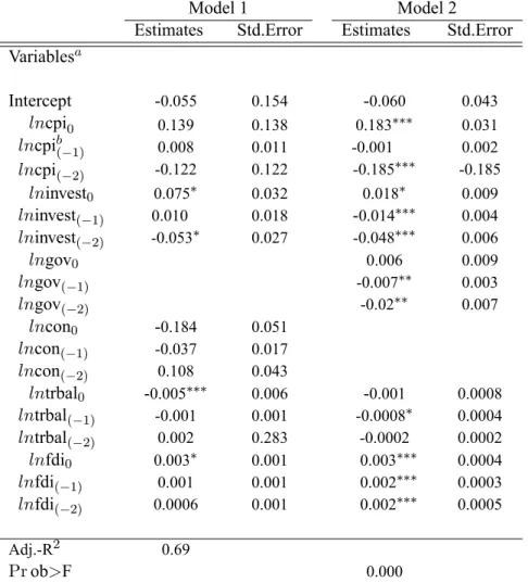
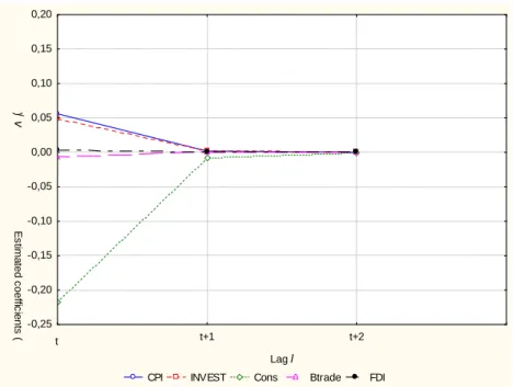
The results presented in Table 3 show that the investment variable has a positive and signi cant impact on economic growth only in the short run. But after one year, this effect becomes no signi cant in the rst model, but changes the sign bluntly in the second model . This result strengthens the analysis we have done above with the Koyck model showing that the total effect (long run multiplier) of investment disappears quickly. The fact that negative effect of investment comes faster in the presence of government expenditures (Model 2) is probably due to the presence of the eviction effect.
The price evolution seems to have a positive effect on economic growth in the current year, but after one year, this effect changes the sign and becomes negative. This result re ects the response function of cameroonian economy. It suggests that an increase of consumption price index will have a negative and signi cant impact on economic growth two years later (hysteresis effect). The Model 2 from Table 3 also shows that the effect of the ratio of government expenditures to GDP on economic growth is negative and signi cant after one year; its current effect is positive but not signi cant. This result shows that government expenditures could have a positive impact on economic growth. However, its interim effect after two years remains negative and equals to -2.1 %20.
Table 3 shows that the ratio of Foreign Direct Investment (FDI) to GDP affects positively and signi cantly economic growth whatever the model used. But in Model 1, this effect is signi cant only for the current period while it's signi cant for all the periods in Model 2. We can observe that FDI is the only variable in our model which doesn't change the sign over the years, this result suggests that this variable could be an important channel to sustain cameroonian economic growth. About trade balance, Table 3 shows that this variable affects negatively economic growth; we also observed that this negative effect comes faster in the presence of consumption. That's why we decided to analyze how the consumption could affect trade balance, thus we ran a simultaneous equation. The rst equation analyzes the impact of consumption on import which is one of the component of trade balance, the second equation analyzes the impact of imports on growth21. By using
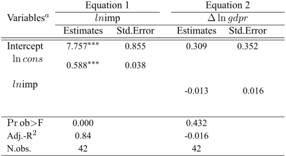
three-stage least squares, we found out that more than half of the increase of consumption is heading toward imports22. In concrete terms, if the consumption increases by
1%, imports will increase by 0.58% (Table 4). This result leads one to conclude that any policy to increase demand reinforces the shortage of trade balance.
19Whatever the considered model, the maximum of lag lenghts doesn't change. 20Pv
l= vrepresents the interim effect. v = 0:006 + ( 0:007) + ( 0:02) = 0:021 21Due to the constraint of identi cation of system of equations, we have used only one explanatory
variable as Wacziarg & Welch (2008).
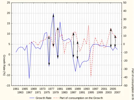
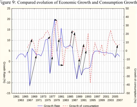
Moreover, Table 3 shows that the effect of consumption is still non signi cant even if the sign becomes postive after two years. To explain this result, we com-puted the contribution of consumption in the growth year per year. The results presented in gure 8 show indeed that during many years, while the evolution of economic growth is positive, the contribution of consumption in the growth23
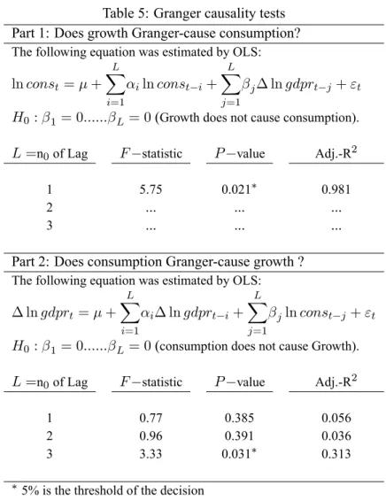
de-creases; we can observe this phenomenon in 1976, 1978, 1980 or in 2004. This result doesn't mean that consumption affects negatively growth, but rather that consumption affects growth with a lag. The gure 9 which displays the growth of consumption and economic growth shows that the sequences of the evolution of consumption growth are the same as the evolution of economic growth but with a lag. To assess econometrically the causal relationship between these two variables (consumption and growth), we performed the Granger causality test24 which the
results are displayed in Table 5.
According to this test, the consumption Granger-causes economic growth after three years but economic growth Granger-causes consumption after one year. We observe that in the couple economic growth-consumption, growth affects consump-tion rst. We could conclude that in the case of Cameroon, consumpconsump-tion follows economic growth.
5 Conclusion
This paper examined how the effects of various variables of economic policy spread on cameroonian growth over the years. With a geometric lag structure, we found out that the speed of adjustment was very high showing that the propagation of the variables' effects of our model disappears quickly; this harms the long-run growth. Thus, we have assessed that 50% of the total effect of all the explanatory variables (investment, index of price, foreign direct investment, consumption, gov-ernment expenditures and balance of trade) is accomplished in less than half of a year.
What ever the model used, we found that investment and foreign direct in-vestment (FDI) had a positive impact on economic growth. The effect of FDI is seemed signi cant only with polynomial distributed lag model. We also found out that in the presence of governement expenditures, the effect of investment on growth is appeared negative after one year due probably to the existence of evic-tion effect. In addievic-tion, our estimaevic-tions showed us that the couple in aevic-tion-growth is indecisive. However, we saw that the impact of in ation on economic growth was generally positive in the current period, but it became negative in the follow-ing years. This result can be explained by the concept of backward-loockfollow-ing rule used by Cagan (1956) concerning the analysis of adaptative expectations models.
23The formula used is:
h
const
gdpt 1 i
100:See the following link www.insee.fr
The suprise result is certainly the non-signi cant impact of consumption on eco-nomic growth after two years, but we found out that this result was probably due to the fact that consumption Granger-causes growth after three years whereas growth Granger-causes consumption after one year.
The main conclusion of this paper is that any economic policy to sustain eco-nomic growth must boost in priority investment and foreign direct investment. Cameroon should pursue policies that stimulate production instead to encourage consumption.
Acemoglu D. & Ventura J., (2002), "The World Income Distribution", The Quarterly Journal of Economics, 117(2): 659-694.
Almon, S., (1965), "The distributed lag between capital appropriations and expenditures", Econometrica, 33: 178–196.
Alt F.L, (1942), "Distributed Lags", Econometrica, 10(2): 113-128.
Balasubramanyam V. N., Salisu M. and Dapsoford D., (1999), "Foreign Direct Investment as an Engine of Growth", Journal of International Trade and Economic Development, 8(1): 27-40.
Barro R.J., (1989), "Economic growth in a cross-section of countries", NBER, Working Paper n 3120.Cambridge: National Bureau of Economic Research.
Bernard A., & Durlauf S., (1995), "Convergence of International Outut Move-ments", Journal of Applied Econometrics, (10): 97-108.
Borensztein E., DeGregorio J. and Lee J-W., (1998), "How Does Foreign Di-rect Investment Affect Economic Growth ?", Journal of International Economics, 45(1): 115-135.
Brander J.A & Dowrick S., (1994),. "The Role of Fertility and Population in Economic Growth: Empirical Results from Aggregate Cross-National Data", Journal of Population Economics, Springer, 7(1): 1-25.
Brunetti A., (1997), "Political variables in cross-country growth analysis", Jour-nal of Economic Surveys, 11(2): 163-190.
Cagan, P., (1956), " The Monetary Dynamics of Hyperin ation", Studies in the Quantity Theory of Money, ed. Friedman, M., Chicago: University of Chicago Press.
Edwards S., (1995), "Exchange Rates, In ation, and Disin ation : Latin Amer-icanExperiences", in Capital Controls, Exchange Rates, and Monetary Policy in the World Economy, ed. by Edwards S. (dir. pub.), Cambridge University Press.
Evans P., (1998), "Using Panel data to evaluate Growth theories", International Economic Review, 39(2): 295-306.
Fomby, T. B., Hill R. C., and Johnson S. R., (1984), Advanced Econometric Methods, New York: Springer.
Frankel J. & Romer D., (1999), "Does trade cause growth ?", American Eco-nomic Review, 89(3) : 379-399.
Fry M., (1978), "Money and Capital or Financial Deepening in Economic De-velopment", Journal of Money, Credit and Banking, 10(4): 464-475.
Fry M., (1980), "Savings, investment, growth, and the cost of nancial repres-sion", World Development, 8(4): 17-27.
Fujita M., Krugman P., Venables A.J., (1999), The Spatial Economy, Cities, Regions and International Trade, Cambridge, Massachusetts : MIT Press.
Gallup J-L, Sachs J.D and Mellinger A.D, (1999), "Geography and Economic Development", International Regional Science Review, 22(2): 179-232.
Gómez V., & Maravall A., (1994), "Estimation, prediction and interpolation for nonstationary series with the Kalman lter", Journal of the American Statistical Association, (89): 611-624
Gujarati N., (2003), Basic Econometrics, 4th ed., McGraw-Hill, Inc. 641p. Gupta Kanhaya L, (1987), "Agregate savings, nancial intermediation and in-terest rate", Review of Economics and Statistics, 69(2) : 303-311.
Jütting J., (2003), "Institutions and Development: A Critical Review," OECD Development Centre, Working Papers 210, OECD.
Knack S. & Keefer P., (1997), "Does social capital have an economic payoff ?", Quarterly Journal of Economics, 112:1251-1288.
Kormendi R.C, Meguire P.G., (1985), "Macroeconomic Determinants of Growth :Cross- Country Evidence", Journal of Monetary Economics, 16(2): 141-163.
Koyck, L. M., (1954), Distributed Lags and Investment Analysis, North-Holland Publishing Company, Amsterdam, The Netherlands.
Krugman P., (1991a), Geography and Trade, Leuven University Press and Cambridge, Massachusetts : The MIT Press.
Lahiri A.K., (1988), "Dynamics of Asian Savings : The Role of Growth and Age Structure", IMF,Working Paper n 49.
Lucas R., (1988), "On the mechanics of economic development", Journal of Monetary Economics, 22(1): 3-42.
Mankiw G., Romer D. and Weil D., (1992), "A Contribution to the Empirics of Economic Growth", Quarterly Journal of Economics, 107(2): 407-437.
Matsuyama K., (1992), "Agricultural Productivity, ComparativeAdvantage, and Economic Growth", Journal of Economic Theory, 58(2): 317-334.
McDowell A., (2004), From the help desk: Polynomial distributed lag models, The Stata Journal, 4(2): 180–189.
Myrdal G., (1957), Economic Theory and Underdeveloped Regions. London : Duck-worth.
Nerlove M. L., (1997), "Growth Models with Endogenous Population: A Gen-eral Framework," (with L. K. Raut).The Handbook of Family and Population Economics, ed. by Rosenzweig M.R. and Stark. O New York: Elsevier Scienti c Publishers.
Presbitero A. F., (2006), "The Debt-Growth Nexus: a Dynamic Panel Data Estimation", Rivista italiana degli economisti, (3): 417-462 .
Romalis J., (2007), "Market Access, Openness and Growth"; NBER, working paper series no. w13048; Cambridge: National Bureau of Economic Research.
Romer P., (1986), "Increasing Returns and Long Run Growth", Journal of Po-litical Economy, 94(5) : 1002-1037.
Romer P., (1990), "Endogenous Technical Change", Journal of Political Econ-omy, 98(5): 71-102.
Solow R. M., (1956), "A contribution to the theory of economic growth", Quar-terly Journal of Economics, 70(1): 65-94.
Swan T., (1960), "Economic Control in a Dependent Economy", Economic Record, 36(73) : 51-66.
Szeto K.L, (2001), An econometric analysis of a production function for New Zealand, Wellington, NZ Treasury, Working Paper 01/31.
Thurman W. N. and Fisher M.E., (1988), "Chickens, Eggs, and Causality, or Which Came First?", American Journal of Agricultural Economics, 70(2): 237-238
Wacziarg R. and Welch K.H, (2008), "Trade Liberalization and Growth: New Evidence", The World Bank Economic Review, 22(2):187-231.
Figure 1: Evolution of growth rate and GDP per capita 1960 1962 1964 1966 1968 1970 1972 1974 1976 1978 1980 1982 1984 1986 1988 1990 1992 1994 1996 1998 2000 2002 2004 2006 Years 400 500 600 700 800 900 1000 1100 US $ ( US $= 20 00 ) -15 -10 -5 0 5 10 15 20 25 % GDP per Capita Grow th Rate
Table 1: Results from the estimations based on the Koyck Transformation
Model 1 Model 2
Estimates Std.Error Estimates Std.Error Variablesa
Intercept -0.194 0.096 -0.220 0.092
lncpi0
lncpi:Total effectb 0.056
0.058 0.020 0.021 0.053 0.059 0.012 0.013 lninvest0
lninvest:Total effect 0.049
0.051 0.027 0.028 0.179 0.198 0.022 0.024 lngov0
lngov:Total effect -0.176
-0.194
0.025 0.0281
lncons0
lncons:Total effect -0.218
-0.226
0.43 0.45
lntrbal0
lntrbal:Total effect -0.006
-0.006 0.002 0.002 0.022 0.0249 0.007 0.008 lnfdi0
lnfdi:Total effect 0.003
0.003 0.002 0.002 0.002 0.002 0.001 0.001 ln gdpr( 1) 0.035 0.035 0.095 0.021 Adj.-R2 Pr ob>F N.obs. 0.58 33 0.000 32.
Durbin h-test: ( Prob>F) 0.153 0.752
Cook W eisberg
test ( Prob>F) 0.153 0.003
Note: signi cant at 10%; signi cant at 5%; signi cant at 1% a)- Except cpi , the other variables are divided by GDP
b)- Estimates and signi cance levels for lagged variables have been calculated by using the delta method.
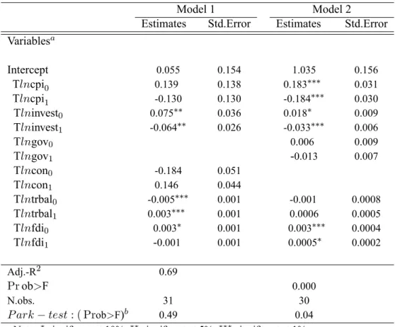
Table 2: Estimated (Almon) Polynomial Coef cients
Model 1 Model 2
Estimates Std.Error Estimates Std.Error Variablesa Intercept 0.055 0.154 1.035 0.156 Tlncpi0 Tlncpi1 0.139 -0.130 0.138 0.130 0.183 -0.184 0.031 0.030 Tlninvest0 Tlninvest1 0.075 -0.064 0.036 0.026 0.018 -0.033 0.009 0.006 Tlngov0 Tlngov1 0.006 -0.013 0.009 0.007 Tlncon0 Tlncon1 -0.184 0.146 0.051 0.044 Tlntrbal0 Tlntrbal1 -0.005 0.003 0.001 0.001 -0.001 0.0006 0.0008 0.0005 Tlnfdi0 Tlnfdi1 0.003 -0.001 0.001 0.001 0.003 0.0005 0.0004 0.0002 Adj.-R2 0.69 Pr ob>F 0.000 N.obs. 31 30
P ark test : ( Prob>F)b 0.49 0.04
Note: signi cant at 10%; signi cant at 5%; signi cant at 1% a)- Except cpi, the other variables are divided by GDP
Table 3: Results from the Regressions using Almon rst order distributed lags
Model 1 Model 2
Estimates Std.Error Estimates Std.Error Variablesa Intercept -0.055 0.154 -0.060 0.043 lncpi0 lncpib ( 1) lncpi( 2) 0.139 0.008 -0.122 0.138 0.011 0.122 0.183 -0.001 -0.185 0.031 0.002 -0.185 lninvest0 lninvest( 1) lninvest( 2) 0.075 0.010 -0.053 0.032 0.018 0.027 0.018 -0.014 -0.048 0.009 0.004 0.006 lngov0 lngov( 1) lngov( 2) 0.006 -0.007 -0.02 0.009 0.003 0.007 lncon0 lncon( 1) lncon( 2) -0.184 -0.037 0.108 0.051 0.017 0.043 lntrbal0 lntrbal( 1) lntrbal( 2) -0.005 -0.001 0.002 0.006 0.001 0.283 -0.001 -0.0008 -0.0002 0.0008 0.0004 0.0002 lnfdi0 lnfdi( 1) lnfdi( 2) 0.003 0.001 0.0006 0.001 0.001 0.001 0.003 0.002 0.002 0.0004 0.0003 0.0005 Adj.-R2 0.69 Pr ob>F 0.000
Note: signi cant at 10%; signi cant at 5%; signi cant at 1% a)- Except cpi , the other variables are divided by GDP
b)- Estimates and signi cance levels for lagged variables have been calculated by using the delta method.
Table 4: Results of Simultaneous equation of Imports and consumption
Equation 1 Equation 2
Variablesa lnimp ln gdpr
Estimates Std.Error Estimates Std.Error
Intercept 7.757 0.855 0.309 0.352 ln cons 0.588 0.038 lnimp -0.013 0.016 Pr ob>F 0.000 0.432 Adj.-R2 0.84 -0.016 N.obs. 42 42
Note: signi cant at 10%; signi cant at 5%; signi cant at 1% a)- We use three-stage least squares
Figure 2:Compared evolution of original and Transformed values' FDI
1960 1962 1964 1966 1968 1970 1972 1974 1976 1978 1980 1982 1984 1986 1988 1990 1992 1994 1996 1998 2000 2002 2004 2006 Years -2E8 -1E8 0 1E8 2E8 3E8 4E8 5E8 6E8 7E8 8E8 US $
Transformed Value (=Original value+11283100)
Figure 3: Compared evolution of original and Transformed values' Trade Balance 1960 1962 1964 1966 1968 1970 1972 1974 1976 1978 1980 1982 1984 1986 1988 1990 1992 1994 1996 1998 2000 2002 2004 2006 Years -6E8 -4E8 -2E8 0 2E8 4E8 6E8 8E8 1E9 1,2E9 1,4E9 US $
Transformed Value (=Original value+499957001)
Original Value
Figure 4:Estimated coef cients by using Koyck Transformation (Model 1)
CPI INVEST Cons Btrade FDI
t+1 t+2 Lagl -0,25 -0,20 -0,15 -0,10 -0,05 0,00 0,05 0,10 0,15 0,20 E s ti ma ted c oeffi c ients ( vl ) t
Figure 5:Estimated coef cients by using Koyck Transformation (Model 2)
CPI INVEST Cons Btrade FDI
t+1 t+2 Lagl -0,25 -0,20 -0,15 -0,10 -0,05 0,00 0,05 0,10 0,15 0,20 E s ti ma ted c oeffi c ients ( vl ) t
Figure 6:Estimated coef cients by using a Polynomial distributed lag (Model 1)
CPI INVEST Cons Btrade FDI
t+1 t+2 Lagl -0,25 -0,20 -0,15 -0,10 -0,05 0,00 0,05 0,10 0,15 0,20 E s ti ma ted c oeffi c ients ( vl ) t
Figure 7:Estimated coef cients by using a Polynomial distributed lag (Model 2)
CPI INVEST GovExp Btrade FDI
t+1 t+2 Lagl -0,25 -0,20 -0,15 -0,10 -0,05 0,00 0,05 0,10 0,15 0,20 E s ti ma ted c oeffi c ients ( vl ) t
Figure 8: Evolution of economic Growth and the contribution of consumption in the growth 1961 1963 1965 1967 1969 1971 1973 1975 1977 1979 1981 1983 1985 1987 1989 1991 1993 1995 1997 1999 2001 2003 2005 2007 Grow th Rate Part of consumption on the Grow th
-15 -10 -5 0 5 10 15 20 25 G rowth Rat e ( %) -50 -40 -30 -20 -10 0 10 20 30 40 50 Par t of c ons umption on the G row th (
Table 5: Granger causality tests Part 1: Does growth Granger-cause consumption?
The following equation was estimated by OLS:
ln const= + L X i=1 iln const i+ L X j=1 j ln gdprt j+ "t
H0 : 1= 0:::::: L= 0 (Growth does not cause consumption).
L =n0of Lag F statistic P value Adj.-R2
1 5.75 0.021 0.981
2 ... ... ...
3 ... ... ...
Part 2: Does consumption Granger-cause growth ?
The following equation was estimated by OLS:
ln gdprt= + L X i=1 i ln gdprt i+ L X j=1 jln const j+ "t
H0 : 1= 0:::::: L= 0 (consumption does not cause Growth).
L =n0of Lag F statistic P value Adj.-R2
1 0.77 0.385 0.056
2 0.96 0.391 0.036
3 3.33 0.031 0.313
5% is the threshold of the decision Note: The data are annual, 1960-2007
Figure 9:Compared evolution of Economic Growth and Consumption Growth 1961 1963 1965 1967 1969 1971 1973 1975 1977 1979 1981 1983 1985 1987 1989 1991 1993 1995 1997 1999 2001 2003 2005 2007 Grow th Rate Grow th of consumption
-15 -10 -5 0 5 10 15 20 25 G rowth Rat e ( %) -50 -40 -30 -20 -10 0 10 20 30 40 50 G rowth of c ons um pti on ( %)
Appendix A: Matrix of correlation ln g dpr ln cpi ln inv est ln g ouv ln co n ln tr bal ln f d i ln g dp 1 ln cpi -0.27 0.12 1 ln inv est 0.04 0.80 -0.003 0.98 1 ln g ouv -0.66 0.00 0.52 0.00 0.39 0.02 1 ln con -0.60 0.00 -0.69 0.00 0.28 0.10 0.91 0.00 1 ln tr bal -0.34 0.05 -0.14 0.42 -0.26 0.13 0.04 0.79 -0.03 0.86 1 ln f d i 0.31 0.07 0.01 0.93 -0.06 0.726 -0.26 0.13 -0.10 0.54 -0.08 0.63 1 Note: signicant at 10%; signicant at 5%; signicant at 1%
Appendix B: Details of Delta Method
The delta method is a more general method for computing con dence intervals. This method takes a function that is too complex for analytically computing the variance (e.g., V arhexp dX n1 + exp dX oicreates a linear approxi-mation of the function, and then computes the variance of the simpler linear func-tion that is used for large-sample inference. While we illustrate this approach with a simple one-parameter example, the approach generalizes readily to the case with multiple parameters.
Let F (x ) be the estimator of interest, for example, F (x ) = Pr(x ) = (x ), where is the cumulative density function for the standard normal distrib-ution. The rst step is to use a Taylor expansion to linearize the function evaluated at b :
F (xb) t F (x ) + b f (x ) where f( ) = F0
( ) is the derivative of F evaluated at . Then we take the variance of both sides of the equation:
V arnF (xb)ot V arnF (x ) + b f (x )o We can easily simplify the right-hand side:
V arnF (x ) + b f (x )o= V ar fF (x )g+V arn b f (x )o = +2 CovnF (x ); b f (x )o
= 0 + V arn b f (x )o+ 0 = ff(x )g2+ V ar b
= ff(x )g2+ V ar b
where we use the fact that , f(x), and F (x ) are constants. To make our example concrete, consider binary probit where Pr(xb) = (xb) and x is any speci c value. The linear expansion is
xb t (x ) + b @ (x )@ where @ (x )@ = x ( x)
Then V arn (x ) + b (x )o = fx ( x)g2V ar b which leads to the symmetric con dence interval"
Pr xb zrnx xb o2V are b # Pr (x ) " Pr xb + zrnx xb o2V are b # Unlike the asymmetric con dence interval based on endpoint transformations,
this con dence interval could include values less than 0 or greater than 1. Next consider a discrete change Pr xab Pr xbb = xab xbb
where xaand xbare two values of x. The linearization is
xab xbb t f (xa ) (xb )g + b @f(xa )@ (xb )g
V arhf (xa ) (xb )g + b @f(xa )@ (xb )g i = V arh b @f(xa ) (xb )g @ i =h@f(xa ) (xb )g @ i2 V ar b =nx2a (xa )2+ x2b (xb )2 2xa (xa ) xb (xb ) o V ar b To evaluate it, we simply replace with b:
Appendix C: Unit root tests of the variables
The unit root tests used in this study are the Augmented Dickey-Fuller tests. The optimal lag length has been chosen using Akaïke criterion. All variables were tested rst to ascertain whether the trend or the constant should be included in the unit root test. We used the the strategy of Dickey & Pantula (1987).
The equation used to perform the Augmented Dickey-Fuller tests is yt= + yt 1+ t +
p
P
j=1
j yt j+ t
pis the lag length .
The null hypothesis: H0 : = 1, presence of unit root
If we don't reject the null hypothesis, we take the rst difference of the series and rerun the test. But, before we perform the ADF test, we must check the optimal lag length, then we run our equation. after that, we verify if the trend and the constant can be included in the unit root tests.
Table 6: Results of Augmented Dickey-Fuller tests Unit Root tests
Variables Lag t-statistic Integration
order Level rst difference order
In ation 1 -1.373 -3.356 1 Investment 1 -3.692 ... 0 Consumption 0 -1.783 -5.110 1 Government expenditures 0 -1.788 -5.767 1 Trade balance 0 -6.460 ... 0 FDI 0 -5.286 ... 0 GDP 1 0.993 -3.771 1