HAL Id: lirmm-01382346
https://hal-lirmm.ccsd.cnrs.fr/lirmm-01382346v2
Submitted on 14 Nov 2016
HAL is a multi-disciplinary open access
archive for the deposit and dissemination of
sci-entific research documents, whether they are
pub-lished or not. The documents may come from
teaching and research institutions in France or
abroad, or from public or private research centers.
L’archive ouverte pluridisciplinaire HAL, est
destinée au dépôt et à la diffusion de documents
scientifiques de niveau recherche, publiés ou non,
émanant des établissements d’enseignement et de
recherche français ou étrangers, des laboratoires
publics ou privés.
Explaining the Results of an Optimization-Based
Decision Support System – A Machine Learning
Approach
Michael Morin, Rallou Thomopoulos, Irène Abi-Zeid, Maxime Léger, François
Grondin, Martin Pleau
To cite this version:
Michael Morin, Rallou Thomopoulos, Irène Abi-Zeid, Maxime Léger, François Grondin, et al..
Ex-plaining the Results of an Optimization-Based Decision Support System – A Machine Learning
Ap-proach. APMOD: APplied mathematical programming and MODelling, Jun 2016, Brno, Czech
Re-public. �lirmm-01382346v2�
Explaining the Results of an Optimization-Based Decision
Support System – A Machine Learning Approach
Michael Morin2,?, Rallou Thomopoulos3, Irène Abi-Zeid1,??, Maxime Léger1, François Grondin4, and Martin Pleau4
1Department of Operations and Decision Systems, Université Laval, Québec, Canada
2Department of Computer Science and Software Engineering, Université Laval, Québec, Canada 3IATE Joint Research Unit, INRA Montpellier, France
4Tetra Tech QI inc., Québec, Canada
Abstract. In this paper, we present work conducted in order to explain the results of a commercial software used for real-time decision support for the flow management of a combined wastewater network. This tool is deployed in many major cities and is used on a daily basis. We apply decision trees to build rules for classifying and interpreting the solutions of the optimization model. Our main goal is to build a classifier that would help a user understand why a proposed solution is good and why other solutions are worse. We demonstrate the feasibility of the approach to our industrial application by generating a large dataset of feasible solutions and classifying them as satisfactory or unsatisfactory based on whether the objective function is a certain percentage higher than the optimal (minimum) objective. We evaluate the performance of the learned classifier on unseen examples. Our results show that our approach is very promising according to reactions from analysts and potential users.
1 Introduction
Decision support systems (DSS) and in particular optimization systems are more and more common in engineering, business, and management environments. Although these systems may be very so-phisticated and powerful in terms of solving complex mathematical models and providing optimal recommendations, more often than not, the users of these systems are skeptical of the results pre-sented. This leads to a resistance and a mistrust with regards to these technologies. More than ever, it is becoming important to explain the solutions of the optimization systems in terms that users and operators can understand, in order to be comfortable in following or challenging the recommenda-tions of these systems. In this paper, we present work conducted in order to explain the results of a commercial software used for real-time decision support for the flow management of a combined wastewater network. This tool is deployed in many major cities and is used on a daily basis. Over the years, our industrial partner has identified the need for explanations of the optimization results which prompted us to define a collaborative project.
?e-mail: [email protected] ??e-mail: [email protected]
Du et al. [1] distinguish between “backward” and “forward” explanations. Backward explanations are past-oriented. They seek reasons in the past (actions, events) that led to the observed situation. Forward explanations are future-oriented. They foresee the future consequences of a possible de-cision. In the present paper, we propose a forward approach which provides explanations for the recommendations of an optimization-based DSS. We apply a machine learning technique to build rules for classifying and interpreting the solutions of the optimization model, namely decision trees. Our main goal is to build a classifier that would help a user (not a researcher or a practitioner from a field related to optimization) to understand why a proposed solution is good and why other solutions are worse.
The paper is structured as follows: Section 2 presents a brief literature review, Section 3 includes the problem background and methodology, Section 4 contains a description of the experiment and the results. We conclude in Section 5.
2 Literature Review
Decision support systems have been around for several decades now. Interestingly, since the 90s, sev-eral studies have pointed out that end users have a low acceptance level of the solutions computed by DSSs [2–5]. These studies have explored, respectively, the importance of feedback about a decision made, the role of cognitive biases in human decision errors, the complexity of the requirements pri-oritization which implies an iterative decision-making process, and the importance of contextual and causal information in forecasting.
However, during the 2000s, studies about the effects of providing explanations on DSS advice acceptance were still extremely rare [6] and they have only recently begun to emerge as an important consideration [7]. In their paper, Du et al. [7] use two machine-learning techniques, namely rough sets and dependency networks, to mine DSS solutions. The mining results are then provided as explanations of the DSS solutions. Both techniques provide different, but not disjoint, results, which are used by the authors to classify the mining results as strong or weak explanations.
In [6], two types of explanations are distinguished: technical ones, tracing the process used to make a forecast, and managerial ones, providing a justification based on the meaning of the forecast. Both types of explanations were estimated to increase decision-makers confidence. This diagnostic is confirmed by Gonul et al. [8]. Based on their review and conclusions, we have built the following three tables which summarize some conclusions about the categories, the roles and the added value of explanations. These are presented respectively in Tables 1, 2 and 3.
3 Background and Methodology
The commercial DSS that we are interested in is a software for real time control and management of a combined wastewater network, provided by our industrial partner. It includes a simulator and an optimizer. The network is made-up of controlled and uncontrolled sections. Based on weather forecasts over a given time period, the simulator simulates the flow in the uncontrolled parts of the network that provide the inputs to the controlled parts of the network. The optimizer’s role is to provide the complete set of control point configurations (decision variables values) that minimizes the overflow cost (objective function) for the considered period. It establishes, based on water flows in the network, a set of instructions that are sent to local stations to regulate flows using sluice gates and pumps. Constraints describe the behavior of the network and the cost function is defined to minimize overflow volumes, storage facility dewatering time, to ensure a balanced hydraulic load distribution throughout the network and to minimize the associated management costs [9]. The provided solution,
Table 1. Categories of explanations
Categories Subcategories Remarks Depending on the content of
explanations
Explanations on the how: system reasoning mechanism (information used, rules, steps)
Explanations on the why: justification of a decision
highlighting the reasons behind the decision
The most efficient for the acceptance of the result provided
Strategic explanations: overview of the whole issue and the stakes tackled by the system
Less used since their obtention is difficult
Depending on the way of providing explanations
On user demand Automated
Intelligent: when a need for explanations is detected by the system
Complex mechanism
Depending on the format in which explanations are presented
Text-based: predefined sentences or combinations following some rules
Natural language-style sentences improve
understanding and acceptance of the system
Multimedia: graphs, pictures, animations
Costly implementation but persuasive and efficient to obtain users’ confidence
Table 2. Roles of explanations
Objectives Benefits for users
Explain a detected anomaly Understand a recommendation Verify that it satisfies the expectations
Solve a contradiction between the users and the system
Provide complementary information Participate in solving a problem (short-term)
Table 3. Added value of explanations
Effects on users Consequences Result Better understanding
Learning
Perform better decision making (accuracy and speed)
Accept the system as logical and thus grounded and useful Follow the logical reasoning
used by the system
Positive perception of the system (ease of use, usefulness,
satisfaction, confidence)
although optimal with respect to the objective function in the model used by the optimizer, can be modified by the end-user.
A solution fully describes, in terms of the values of the decision variables, the state of the con-trolled section of the network. Decision variables determine, in particular (but not exclusively), the positions of all the control gates regulating the wastewater system flow management. These can be closed or open to a certain extent.
3.1 Methodology
Given an optimal solution to an optimization problem provided by solving a mathematical program, in this case a minimization problem, we wish to enable an end-user to understand which characteristics of a solution render it more or less suitable (satisfactory) from the perspective of the decision s/he has to make. From a single objective optimization perspective, a solution that is optimal minimizes a predefined and accepted objective function while being feasible, i.e., while respecting a set of pre-defined constraints. We employ the term satisfactory to describe a feasible solution that is a suitable decision in the context where a mathematical program is used as part of a DSS. An optimal solution is of course satisfactory. However, some satisfactory solutions might be suboptimal.
Suppose, for instance, that a small increment δ in the objective function value is tolerable. Any feasible solution x with an objective value f (x) that is not worse than f (x∗) + δ , i.e., f (x) ≤ f (x∗) + δ , is said to be satisfactory. Although x is not optimal, it is a suitable decision with respect to that criterion.
We therefore need a methodology to characterize the satisfactory solution set, using simple rules, in order to allow a DSS user to understand the following:
1. why a solution (including the optimal one) is satisfactory; and
2. why a given change to an optimal solution might produce a solution that is worse, or potentially catastrophic in practice.
If a user is not satisfied with the optimal solution initially provided by the DSS for a number of possible reasons, including the fact that it does not intuitively make sense to her/him, the rules (explanations) would allow her/him to understand which decision variables can be modified (and how) before the DSS can re-optimize and return a new satisfactory solution.
We chose to use decision trees to produce (learn) such a simple set of rules to characterize the set of satisfactory solutions. This is similar to the approaches in [7], albeit in a different context and on bigger-size data sets.
3.2 Decision trees and the classification of satisfactory solutions
Decision trees are a widely used machine learning technique. In the next subsections, we briefly present machine learning and decision trees as we applied them to the problem of characterizing the set of satisfactory solutions.
3.2.1 Machine learning
(Supervised) machine learning is the art of learning by examples [10]. A learning algorithm is pro-vided with a training set S of examples. Each example in set S is a pair (x, y) where x is an input and yis an output. The output can be a class, a real number, or it can have a structure [11]. When x ∈ Rn and y ∈ {True, False}, we have a binary classification problem. We call the entries in x the features and y the class.
A solution to the binary classification problem is a function h, called a classifier, that takes an input x ∈ Rnand that outputs y ∈ {True, False}. A learning algorithm builds a classifier h using the set S, i.e., known pairs (x, y) of features and class (training phase). Once built, the classifier can be used to compute an output class y given an unseen vector of input features x (testing phase). In this paper, we formulate the problem of recognizing satisfactory solutions from unsatisfactory ones as a binary classification problem.
3.2.2 Decision trees
A decision tree [12] is a classifier in the form a tree structure. Classifiers can be either white box or black boxmodels. We chose to use decision trees since a decision tree is a white box and interpretable model made of simple decision rules. It takes x as an input, and it outputs a class y. The nodes of the tree are either decision nodes or leaves. A decision node corresponds to a branching rule based on the value of a single input feature. A leaf node is assigned a prediction class.
In the training phase, a decision tree is built in a greedy fashion by the learning algorithm. The examples of the training set S, i.e., the known examples, start at the root of the tree. A first branching rule is applied at the root on the training examples. The learning algorithm chooses the branching rule that best partitions the training examples according to a heuristic. All examples x that respect the branching rules take the left path. All other examples take the right path. At the next level, a new decision node is created for each partition and two branching rules are selected according to the partitioning heuristic. Branching stops when all the examples of a partition belong to the same class. Other stopping criteria to manage the height of the tree can be used. In that case, not all the examples in a partition that reach a leaf will have the same class and the value of the leaf can be set to the majority class.
In the testing phase, an unseen example x, i.e., an example for which y is unknown, follows a path from the root to a leaf. The example is tested against each decision rule. If it respects the rule, it branches left, otherwise it branches right. The predicted class is that of the reached leaf.
3.2.3 Learning to recognize satisfactory solutions
As mentioned previously, each node of a decision tree, except the leaves, is a branching rule. A path from the root to a leaf can be seen as a rule describing the satisfactory solution set. We first learn a decision tree (training phase). Later on, this decision tree is used to determine whether a solution is satisfactory or not (test phase). Furthermore, since a decision tree is interpretable, it provides a set of
rules characterizing satisfactory solutions. We next describe the process used to generate the set S of training examples that can be used for learning.
Assume that an optimal solution has been provided by the DSS and that a satisfactory criterion has been determined. We generate set S by simulating a sufficiently large number of modifications of the optimal solution. Simulating a modification consists in randomly fixing a decision variable’s value. After each simulation, we evaluate the value of the solution according to the chosen criterion that discriminates between satisfactory and unsatisfactory ones. We store in S, the value of all decision variables along with the class of the newly generated solution: satisfactory (true) or not (false). Finally, we learn one or more decision trees on S.
4 Experiment
In order to demonstrate the feasibility of the approach to our industrial application, we generated a large dataset of feasible solutions and classified them as satisfactory or not based on whether the objective function is a certain percentage higher than the optimal objective. We then used a small subset of these solutions to learn a classifier. The small subset used for learning is the training set (S). We evaluated the performance of the learned classifier on the remaining unseen examples. We provide the details on the data we generated for the experiment in the next subsection.
4.1 Data preparation
In order to learn the characteristics of the satisfactory solution set, we first obtained an optimal solution to a problem instance using the optimizer of the DSS developed by our partner. The weather forecast, the simulation results, and the provided optimal solution belong to a real use-case scenario.
Starting from the optimal solution, we generated 10,000 feasible solutions by simulating a single modification of one of the decision variables by the end-user. Each solution of the dataset used for the experiment is generated as follows:
• one of the decision variables is chosen and modified randomly;
• the objective value of the solution resulting from the perturbation of that single control point is reevaluated.
The resulting dataset contains the values of all the variables of the optimization model for all the gen-erated solutions along with their objective value. We then filter the dataset to keep only the variables that can have an explanatory significance for the end-user. The identification of these variables was performed by the domain experts. We excluded all the variables that are used as components of the objective function. We then assigned a class to each solution. For the purpose of the experiment, we assume that a solution is nonsatisfactory if and only if its objective value exceeds by 5% (or more) the optimal value.
In the next subsection, we present, the results of our methodology when used jointly with decision trees.
4.2 Decision trees and their predictive accuracy
All decision tree experiments are conducted using scikit-learn [13], a machine learning library for the Python programming language.
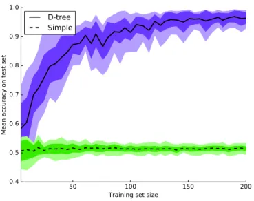
Figure 1 shows the learning curve we obtain on our industrial instance. Most learning algorithms for decision trees are greedy algorithms. Scikit-learn’s learning algorithm for decision trees makes no
50 100 150 200 Training set size
0.4 0.5 0.6 0.7 0.8 0.9 1.0
Mean accuracy on test set
D-tree
Simple
Figure 1. Learning curve: Mean accuracy of the learned decision trees (solid curve) and of the simple classifiers (dashed curve) on the test set against various training set sizes with standard deviation in blue and green shading and upper and lower bounds in light blue and light green
exception. In order to evaluate the predictive accuracy of decision trees in our context, we partitioned the dataset into a training set S and a test set. Some partitions might be more or less satisfactory for learning. We aggregated the results of 10 different partitions. We generated the curve of Figure 1 by varying the size of the subset of S used for training. For each subset of S, ranging in size from 5 to 200 training examples (for a total of 40 subset sizes), we learned 10 different trees and aggregated the results. Each tree was tested against the 9,800 remaining examples in the test set. Using such a large test set enables us to verify whether a decision tree learning algorithm can generate rules to characterize the satisfactory solutions space of our industrial problem instance by accessing a few training examples only. The solid curve plots the average predictive accuracy of the decision trees against the size of the training subsets used for learning. The blue shaded region shows the standard deviation. The light blue shaded region shows the minimal and the maximal predictive accuracy encountered for each size of subset of the training set. The dashed curve plots the average predictive accuracy achieved by the mean of simple classifiers generating their prediction using the distribution of the classes in the training set. The standard deviation region and the region of the bounds of the simple classifiers are displayed in green.
The decision rules learned by the decision trees were validated by experts from the application field. The tendency of the learning algorithm was to choose high impact control points (decision variables) in its first few decision rules.
5 Conclusion
In this study, we have proposed an approach using decision trees to explain the results of a commercial software used for real-time decision support for combined wastewater system flow management. Our
solution allows analysts to identify the main criteria that influence the DSS outcome, and helps users in understanding the rationale behind the DSS’s recommendations. The rationale supporting this approach consists in classifying the space of solutions according to some criterion that characterizes the performance of the solutions proposed by the DSS.
We plan to explore several directions in the next stages of this work. First, we will identify “optimal” sizes of the training set and tree depths, allowing for both a good learning quality and a reasonable computing time. Moreover, the robustness of the method will be tested based on the following factors: on the one hand, the number of variables taken into account, in particular for increased numbers of predictive variables; on the other hand, the proportion of positive examples composing the training set. Finally, we plan to experiment our approach on other kinds of learning algorithms, also able to compute interpretable classifiers, with the long-term objective of providing users with arguments expressing the learnt rules.
References
[1] G. Du, M. Richter, G. Ruhe, An explanation oriented dialogue approach and its application to wicked planning problems, Journal of Computing and Informatics 25(2–3), 223 (2006)
[2] F.D. Davis, J.E. Kottemann, Determinants of decision rule use in a production planning task, Organizational Behavior and Human Decision Processes 63(2), 145 (1995)
[3] B. Kleinmuntz, Why we still use our heads instead of formulas: Toward an integrative approach, Psychological Bulletin 107(3), 296 (1990)
[4] L. Lehtola, S. Kujala, Requirements prioritization challenges in practice, in Proc. of the 5th International Conference on Product Focused Software Process Improvement (PROFES)(2004), pp. 497–508
[5] J.S. Lim, M. O’Connor, Judgmental forecasting with time series and causal information, Inter-national Journal of Forecasting 12(1), 139 (1996)
[6] M. Lawrence, L. Davies, M. O’Connor, P. Goodwin, Improving forecast utilization by providing explanations, in Proc. of the 21st International Symposium on Forecasting (ISF) (2001) [7] G. Du, G. Ruhe, Two machine-learning techniques for mining solutions of the ReleasePlanner™
decision support system, Information Sciences 259, 474 (2014)
[8] M.S. Gönül, D. Önkal, M. Lawrence, The effects of structural characteristics of explanations on use of a DSS, Decision Support Systems 42(3), 1481 (2006)
[9] M. Pleau, H. Colas, P. Lavallée, G. Pelletier, R. Bonin, Global optimal real-time control of the Quebec urban drainage system, Environmental Modelling & Software 20(4), 401 (2005) [10] C.M. Bishop, Pattern Recognition and Machine Learning (Springer, 2006)
[11] G. Bak˘ır, T. Hofmann, B. Schoölkopf, A.J. Smola, B. Taskar, S.V.N. Vishwanathan, eds., Pre-dicting Structured Data(MIT press, 2007)
[12] L. Breiman, J. Friedman, R.A. Olshen, C.J. Stone, Classification and Regression Trees (Chap-man and Hall, 1984)
[13] F. Pedregosa, G. Varoquaux, A. Gramfort, V. Michel, B. Thirion, O. Grisel, M. Blondel, P. Pret-tenhofer, R. Weiss, V. Dubourg et al., Scikit-learn: Machine learning in Python, The Journal of Machine Learning Research 12, 2825 (2011)