Computer-aided thermodynamics modeling of a pure substance

1)

Computer-Aided Thermodynamics Modeling

of a Pure Substance

by

Jose L. Perez

B.S.M.E., University of Puerto Rico, MayagUez (1992)

Submitted to the Department of Mechanical

Engineering in Partial Fulfillment of the

Requirements for the Degree of

MASTER OF SCIENCE in MECHANICAL ENGINEERING

at the

MASSACHUSETTS INSTITUTE OF TECHNOLOGY

May 1995

© 1995 Massachusetts Institute of Technology All rights reserved.

Signature of Author

Certified by

rtment of Mechanical Engineeng

- May 12, 95

A

~ ~~

/-

-.__ - sdAl-.

? Pe6fessor Joseph L. Smih, Jr.

Thesis Supervisor

Accepted by

MASSACHUSETTS INSTITUTE OF TECHNOLOGY

Professor Ain A. Sonin Chairman, Graduate Committee Department of Mechanical Engineering AUG 311995

LIBRARIES

-Computer-Aided Thermodynamics Modeling

of a Pure Substance

by

Jose L. Perez

Submitted of the Department of Mechanical

Engineering in partial fulfillment of the

requirements for the degree of

Master of Science in Mechanical Engineering

Abstract

This thesis consists of three parts. First a Computer-Aided Thermodynamic (CAT) methodology is developed that enables modeling of a Pure Substance. The second part of the thesis develops the corresponding cT-based software for the modeling of steam as a Pure Substance. Finally, in part three the cT source code is presented, and some trial problems are analyzed using the software.

The foundation for the CAT methodology was developed here at the Massachusetts Institute of Technology (MIT) by Professor Joseph L. Smith, Jr. and Dr. Gilberto Russo in Russo's 1987 doctoral thesis A New Methodology of Computer-Aided

Thermodynamics. The resultant CAT algorithm and software was later refined and

in-corporated into MIT's Athena Project by Chun-On Cheng, graduate student at MIT. Mr. Cheng used C as programming language in the X-Windows environment. More recently, Oscar C. Yeh, working as an undergraduate research student at MIT translated the CAT source code into the cT language. The choice of cT as the source code language means that the CAT program is now portable across computer systems such as UNIX, Microsoft-DOS, and Apple Macintosh.

This thesis, built on the aforementioned work, presents the algorithm and corre-sponding source code for analysis of steam as a Pure Substance within the framework of the CAT methodology. The result is the addition of a new Steam Element to the array of choices previously available in the CAT program. The Steam Element is capable of modeling the behavior of steam at its liquid, liquid-vapor, and vapor states. Although the basic algorithm can be used for any substance that typically undergoes phase changes, the current code runs for steam, based on the equations of state for steam developed in Steam

Tables, by J. Keenan, et al. (1969).

Thesis Supervisor: Dr. Joseph L. Smith, Jr. Title: Ford Professor of Mechanical Engineering

To my wife, Carmen Enid, my mother, Alba Nydia and my soon-to-be-born daughter, Laura Enid.

Acknowledgments

I would like to express my gratitude to the people who helped, directly or indi-rectly, to the fruition of this thesis. Among them, Professor Joseph L. Smith, Jr., for his insight and assistance in helping me understand the CAT methodology and its concepts. Also, Professor Adeboyejo (Ade) Oni, for his enthusiasm in the initial stages of this pro-ject.

I would also like to thank the people who I call "the computer guys", Tom Cheng and Oscar Yeh, who programmed CAT in the C and cT languages, respectively. They were always available when I required their technical assistance.

For the emotional assistance throughout my graduate school years I have to thank my wife, Carmen Enid. She celebrated my good moments and consoled me during the bad times. Te quiero mucho, Dindita. My mother, Alba Nydia, was also a source of emotional (and sometimes financial) support during my undergraduate years at Maya-gtiez. Gracias, Mami.

Finally, I wish to acknowledge the financial support provided by General Electric for my first year of studies at MIT; the support from the Naval Undersea Warfare Center (NAVUNSEAWARCENDIV) for my third semester; and the financial assistance ar-ranged for my last semester at MIT by Margo Tyler, Assistant Dean at the Graduate

Table of Contents

Abstract ... 3 Dedication ... 5 Acknowledgments ... 7 Table of Contents ... 9 List of Figures ... 11

Part I:

Conceptualization and Formulation

1 Preamble 1.1 Background ... 14

1.2 Basis for Method ... 15

1.3 cT-Based Application Development ... 16

2 CAT Methodology 2.1 Overview ... 17

2.2 Modeling Concept ... 17

2.3 CAT Elements ... 18

2.4 Topology Matrices ... 19

2.5 Derivation of System Equations ... 21

2.6 Stiffness Matrix Elements ... 22

2.7 Reversible Process ... 24

3 Pure Substance Element Modeling 3.1 Overview ... 27

3.2 Equations for Water Vapor and Liquid Regions ... 27

3.3 Equations for Water Liquid-Vapor Mixture (Saturation) ... 32

3.4 Stiffness Matrix Expressions for Water Vapor and Liquid Regions ... 34

3.5 Stiffness Matrix Expressions for Liquid-Vapor Mixture (Saturation) .... 35

Software Development

4 Introduction

4.1 cT as the Development Language ... 44

5 The CAT Software 5.1 Organization ... 45 5.2 Mesh Creation ... 45 5.3 Input Routines ... 46 5.4 Computational Algorithm ... 48 5.5 Solution Presentation ... 51 5.6 Relations Database ... 52

5.7 Graphical Interface Routines ... 52

6 Steam Element Software Development 6.1 Input Routine ... 53 6.1.1 Known Quality ... 53 6.1.2 Unknown Quality ... 54 6.2 Steam Functions ... 58 7 Conclusion 7.1 Potential Extension ... 63 7.2 Closure ... 64

Part m:

Appendices

Appendix A Running CAT A.1 Using cT and CAT.t ... 66

Appendix B Sample CAT Runs B. 1 Modeling a Problem in CAT ... 67

B.2 Sample Problems Using the Steam Element ... 69

Appendix C Source Code C.1 Steam Element Computer Code ... 78

C. 1.1 Modified Units ... 78 C. 1.2 New Units ... 120 Appendix D Bibliography Bibliography... 139 Biographical Note ... 140

Part II:

List of Figures

2.1 Isolated system ... 18

2.2 Mesh of interconnected elements ... 20

2.3 Isolated system with mechanical matching element ... 24

3.1 P-v-T plot from equation (3.1) ... 40

3.2 P-v-T plot from equation (3.1), first half of saturated region ... 41

3.3 P-v-T plot from equation (3.1), second half of saturated region ... 42

5.1 CAT initial screen ... 46

5.2 Flowchart, unit num erical ... 50

5.3 CAT results screen ... 51...5

6.1 Input routine decision tree (known quality) ... 56

6.2 Input routine decision tree (unknown quality) ... 57

B. 1 Sample thermodynamic problem, piston cylinder apparatus ... 67

B.2 CAT mesh for sample problem ... 68

B.3 CAT solution to sample problem ... 68

B.4 CAT mesh for problem 1 ... 71

B.5 CAT solution to problem 1 ... 71

B.6 CAT mesh for problem 2 ... 72

B.7 CAT solution to problem 2 ... 72

B.8 CAT mesh for problem 3 ... 73

B.9 CAT solution to problem 3 ... 73

B.10 CAT mesh for problem 4 ... 74

B.11 CAT solution to problem 4 ... 74

B.12 P vs. V plot, problem 4 ... 75

B.13 P vs. Tplot, problem 4 ... 75

B.14 CAT mesh for problem 5 ... 76

B.15 CAT solution to problem 5 ... 76

B. 16 CAT mesh for problem 6 ... 77

1 Preamble

1.1 Background

The thermodynamic behavior of a system can be modeled as set of mechanical work transfer interactions and thermal heat transfer interactions occurring within the sys-tem. These interactions occur among smaller subsystems with defined thermal and me-chanical properties. The Computer-Aided Thermodynamic (CAT) algorithm is based on this approach. Instead of devising a particular solution procedure for analysis of any given thermodynamic system, the CAT methodology automates the problem setup in a manner which can easily be solved by a numerical computational algorithm. The au-tomation of problem setup is done by decomposing the thermodynamic system into

ele-ments that interact among them by means of mechanical and/or thermal interconnections.

Each element has its own set of properties, and its behavior is defined by an equation of state (also referred to here as a constitutive relation). The interconnections define the thermodynamic interaction between elements.

The foundation for the CAT methodology was developed here at the Massachusetts Institute of Technology (MIT) by Professor Joseph L. Smith, Jr., and Dr. Gilberto C. Russo. The CAT algorithm, and corresponding computer software was for-mally presented in Dr. Russo's 1987 doctoral thesis "A New Methodology for

Computer-Aided Thermodynamics". The original CAT version was a 1.5-megabytes,

FORTRAN-77 computer program, running under the UNIX/ULTRIX operational system. More re-cently, MIT graduate student Chun-On Cheng updated the computer code to a C com-puter program, and MIT undergraduate student Oscar C. Yeh translated the C code into cT, a portable language across computer operating systems (UNIX, MS-DOS, Apple Macintosh). Currently, the C version of CAT is being used by MIT undergraduate stu-dents as part of the 2.40 Thermodynamics course.

This thesis builds on the past work to produce an algorithm, and corresponding software code, for modeling and analysis of steam as a pure substance. Prior to this work, the CAT algorithm was only able to model substances as single-phase ideal gases. With the addition of the steam element, CAT is now able to model a pure substance, such as water, an its behavior in the liquid, liquid-vapor and vapor states. The new steam

ele-rium problems as well as reversible process problems. Although the algorithm can be used with any substance that typically undergoes phase changes, such as Refrigerant-12 for instance, the current version of the CAT runs with water, using the equations devel-oped by J. Keenan, et al., in Steam Tables (1969).

1.2 Basis for Method

The CAT software consists of a graphical interface that allows the user to model a given thermodynamic system as an assembly or mesh of interconnected elements. The interconnections determine the type of interactions between elements: whether two ele-ments are thermally connected (i.e., equal temperature at equilibrium) or mechanically connected (i.e., equal pressure at equilibrium). After modeling the given thermodynamic system, the computer program performs the necessary steps to generate a solution, namely, setup of equations, solving of equations by numerical methods, and presentation of results.

The equations are established depending on the type of process involved. When modeling final equilibrium problems, we seek to determine the final state of a system given certain initial conditions. This is achieved by generating force-balance and energy-balance equations. The force energy-balance equation establishes that at equilibrium, all me-chanically connected elements will have a resultant zero force at each node. A node is the point of connection between two elements, for example, it can be though of as an adi-abatic moveable wall separating two gases. At equilibrium, the net force on this wall is zero, meaning the two gases have come to the same pressure. The energy balance equa-tion establishes that all mechanical or thermally connected elements will have the same energy level, mechanical or thermal. For the example of the two gases separated by a wall, if connected by a thermal interconnection only, it would mean having a fixed, ther-mally conductive wall. At equilibrium these two gases will have the same temperature. When modeling reversible process problems, the energy balance equation is replaced by an entropy balance equation. A mechanical matching element is introduced to ensure mechanical equilibrium at every step of the process (quasi-static process), so that the net entropy change is zero.

These equations are solved for the independent variables, namely temperature and nodal displacement at each element. CAT uses a Newton-Raphson algorithm to solve the

equations. The Newton-Raphson method requires that derivatives for all equations, with respect to each independent variable be calculated. These are programmed in the CAT source code. At each iteration CAT performs several checks to ensure the iteration pro-cess is headed in the right direction. If any of the variables drift from the expected solu-tion (e.g., negative temperatures or volumes) CAT takes corrective acsolu-tion in order to pro-duce a solution that will not violate the laws of thermodynamics.

Finally, the results are displayed to the user in a tabular form, listing the proper-ties for each element along with the initial and final states of the major properproper-ties. In the reversible process case, there is even a function that will plot the property values as they changed from initial to final conditions.

The new steam element was added to couple with the CAT program without any major changes to the basic algorithm. As such, it equips the CAT program with the nec-essary functions and routines to effectively model the behavior of steam as a pure sub-stance, taking into account changes of the substance phase which are typical of steam ap-plications.

1.3 cT-Based Application Development

The choice of cT as the development language satisfied the following functional requirements:

* modular programming

* portability across computer systems * dynamic memory allocation

* capability for graphical interface programming.

cT is an integrated programming environment developed in the Center for Design of

Educational Computing at Carnegie Mellon University. It is designed to help develop interactive applications for modern computers, and the programs can run without change on Macintosh, MS-DOS, and UNIX with X11. For these reasons, cT was found suitable for the development of CAT and the steam element algorithm extension.

2 CAT Methodology

2.1 Overview

CAT was established in an attempt to standardize problem solving in thermody-namics to a larger extent than it is currently possible. Solutions to thermodynamic prob-lems have typically been ad hoc, equations devised for a specific problem were valid for that type of problem only. Even though solutions to thermodynamic problems are often derived from energy balance equations, and the application of the First and Second Laws of Thermodynamics, once these governing equations are simplified to suit a particular problem, their generality is lost. CAT preserves this generality at the expense of a few extra steps in calculations, but in a manner that can easily be handled by a computer. 2.2 Modeling Concept

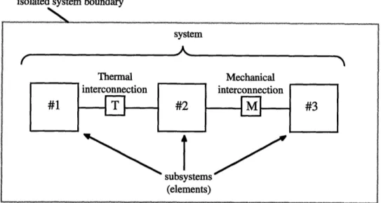
A thermodynamic system is represented as an isolated system composed of inter-connected subsystems, as shown in Figure 2.1. Each subsystem is described by a speci-fied list of equilibrium properties and equations of state (constitutive relations). Each of the subsystems is modeled as being capable of one or more energy transfer interactions. Currently, CAT support two types of energy transfer between subsystems (elements). They are: heat transfer, due to a temperature difference (represented by a "T" symbol, for thermal interaction) and work transfer, due to boundary forces and related displacements (represented by a "M" symbol, for mechanical interaction).

In addition to allowing energy transfer between elements, the interconnections imply that at equilibrium, certain conditions will exist. Specifically, a thermal intercon-nection implies temperature equality between the two interconnected elements at equilib-rium. In Figure 2.1, the temperature of element will be the same as the temperature 2, upon reaching system equilibrium. A mechanical interconnection means force or pres-sure equality between the two interconnected elements at equilibrium. In Figure 2.1, the pressure of element 2 will be the same as the pressure of element 3, upon reaching system equilibrium. The resultant force at the boundary (represented by the "M") will be zero.

isolated system boundary

system

2,

Figure 2.1: Isolated System

2.3 CAT Elements

Elements are used to model physical entities. An element is defined by the fol-lowing attributes:

* a set of constitutive relations * a set of independent properties * a set of dependent properties.

The elements modeled by CAT (not including the Pure Substance/Steam element, which is the focus of this thesis and is treated separately in Section 3) and their attributes are tabulated below.

Element - Constitutive Relations

Pressure/Force Energy Entropy

Thermal reservoir - Any Uto keep T constant

-Thermal capacity _ U = mcv T S = mc InT

Pressure reservoir F=-PA U = Fdl

Ideal Spring F = k(L- ) U = k(L -L )2 _

Ideal gas P = mRT/VU = mc~T S=mRln V + mcl In T

Table 2.1: Elements and their constitutive relations subsystems

(elements)

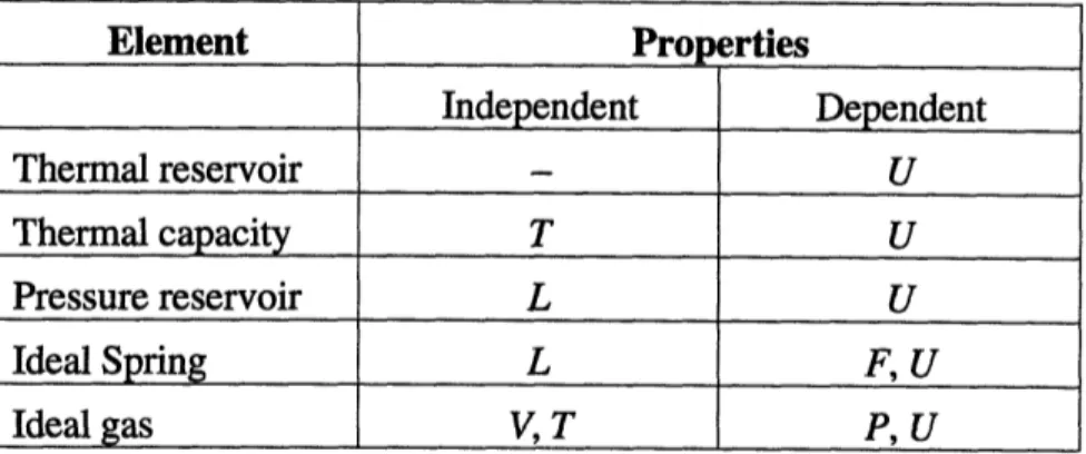
Element Pro erties Independent Dependent Thermal reservoir - U Thermal capacity T U Pressure reservoir L U Ideal Spring L F, U Ideal gas V, T P, U

Table 2.2: Elements and their properties

2.4 Topology Matrices

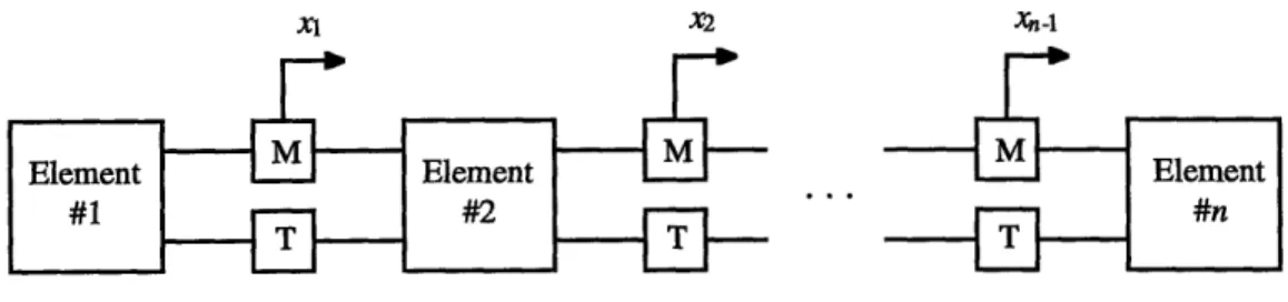
In order to systematically describe the arrangement of elements and their inter-connections for any given problem, CAT generates topology matrices, one for each type of interconnection involved. Consider a mesh of interconnected elements as shown in Figure 2.2. When the mesh has been completely initialized, all the physical and initial state properties are specified for each element. Moreover, the interconnections are inac-tive or "frozen" prior to the simulation and equation solving. The mechanical topology matrix is defined as follows:

TM =

Oal

(2.1)

where

m = number of mechanical interconnections in the mesh

n = number of elements in the mesh

{-1 if elementj is connected to mechanical interconnection i

a'=}O = otherwise.

... an

I

... an

Similarly, the thermal topology matrix is defined as

...

TT = (2.2)

where

t = number of thermal interconnections in the mesh

n = number of elements in the mesh

pi =I if element j is connected to thermal interconnection i 0 otherwise.

We use the following notation:

* Parameters with superscripts are for element or local state parameters; the superscript is the element number. For instance, V1is the volume of element one.

* Parameters with subscripts are for system or global state parameters; the subscript is the interconnection number. For example, x is the boundary (nodal) displacement associ-ated with interconnection one.

* Parameters with superscripts and subscripts are for element nodal parameters. Here the superscript and the subscript are the element and the interconnection that share that node.

F2 is the force exerted by element number two on mechanical interconnection number

one.

Xl X2 Xn 4

Figure 2.2: Mesh of interconnected elements

The continuity of mechanically interconnected elements relate element nodal dis-placements to the volume at each element. For the mesh in Figure 2.2

VI _V =V' _{i nitial} +Ax,

Vi = Viitial + A(xi- xi-) (i = 2,...,n- 1) (2.3)

Vn = Vin~,jal + Axn-,.

There is no continuity requirement, however, for thermal interconnections.

2.5 Derivation of System Equations

Once all elements have been initialized and the topology matrices generated, CAT proceeds to establish the main system equations. These equations describe the behavior of the entire, isolated system by summing their respective force and energy constitutive relations. The solution to these equations constitute the final equilibrium state of the system. For the case of reversible process, the energy equation is replaced by an entropy summation equation. The final equilibrium case is discussed first. For simplicity of pre-sentation, let us consider the case of a system with a single thermal domain. A thermal domain is a portion of the system that consist of thermally interconnected elements. These elements may have different initial temperatures, but at equilibrium they all have the same temperature.

Let Fi be the resultant nodal force residual at the ith mechanical interconnection

and Ej be the energy at the jth element. Then the global system equations are

n

tI F

j

_{; i=l,2,...,n}

_-1

~~~~~~j=l~~~~ ~(2.4) n RE=

E

-

EO.

(2.5) j=l

There is a total of n nonlinear, simultaneous equations. When the residuals R. and RE are zero, mechanical and thermal equilibrium is reached. Our goal is to find the values of xi and T, such that all residuals are zero. This is accomplished by using the Newton-Raphson method for nonlinear equations. We linearize equations (2.4) and (2.5) by

=R~ -0 =, + ·A. 1,2, ..i= ,n-1 (2.6)

ARE

=E

dE

j=1 I~ d

These set of linear equations can be rewritten as the matrix form

dxl

dJI

dx1 dRE dx, dR, dXn-i dxn-1 tn-1 . O~Xn_dRE ₁ aXn-I dRI JT

d-1

AT dRE d3T AXn- A-1 LAT ARE (2.7) (2.8)

The square matrix (n x n) on the left hand side of equation (2.8) is known as the stiffness matrix. The column vector on the right hand side contains the force and energy residu-als. By finding the inverse of the stiffness matrix (by means of a Gauss elimination al-gorithm) we can solve the equation for the nodal displacements and the system tempera-ture. This is done in successive iterations, where the variables of interest, xi and T, are

updated as

(2.9)

xi

k+ = x

-A -'

(i = 1,2,...,n-1)

Tk+l = Tk _ ATk .

When the system reaches equilibrium state, all nodal forces are zero and all thermally connected elements reach a common temperature; the residuals vector is zero.

2.6 Stiffness Matrix Elements

The entries of the stiffness matrix in equation (2.8) are given by the following ex-pressions dR n dFk - = ,_ _ dxj k=1 dxj dR, n dFk

dT

k=l dT X 0/,kV k 'I i JVk (AC) Ek1 a = E x k P ~P k a'T =kA

dT

(2.10) (2.11)

dRE dE = dE dVk dEk (Ak) (2.12)

dx1~~dx ~dVk

d

--x dV k _jki2.2

dRE n dEk (2.13)

8T k=1

dT'

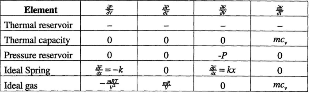
The terms --A, -- , --, and -S in equations (2.10) through (2.13) can be derived for each element from the element constitutive relations (Table 2.1). Notice that the partial derivatives in the stiffness matrix are also dependent on the mesh topological informa-tion. Typically, many of the terms in the above summations are zero from the mesh topology alone. Table 2.3 lists the terms a, ~, ., and for each element in CAT.

Table 2.3: Expressions for Stiffness Matrix

A note about the thermal reservoir element is in order. When there is a thermal reservoir in the mesh, the system temperature is fixed by the thermal reservoir temperature. Since the thermal reservoir acts as an energy source (or sink), energy in the mesh is no longer conserved and the energy balance equation can be deleted from our system of equations. Temperature is no longer an independent variable, and the stiffness matrix loses its last row and column. The stiffness matrix becomes a n-l square matrix and the matrix equa-tion (2.8) reduces to dR, dR, F _ _ '.___ = dR , .Ax , (2.14) 1 .. -I An-1

Element

d __ r Thermal reservoir - - -Thermal capacity 0 0 0 mc, Pressure reservoir 0 0 -P 0 Ideal Spring = -k 0 f = kx 0 Ideal gas - v_ - 0

mcv

2.7 Reversible Process

The solution of a reversible problem is built upon the final equilibrium solution methodology. For an isolated system to undergo a reversible process, the system must go from an initial state to a final state through a continuum of equilibrium states, i.e., at each intermediate state, the system must be in neutral equilibrium. In CAT, this is accom-plished by introducing a new element that ensures mechanical equilibrium of the system during the reversible process. We call this element the mechanical matching element since its job is to match the residual force of the system, thereby attaining mechanical equilibrium at each step of the process.

Figure 2.3: Isolated system with mechanical matching element

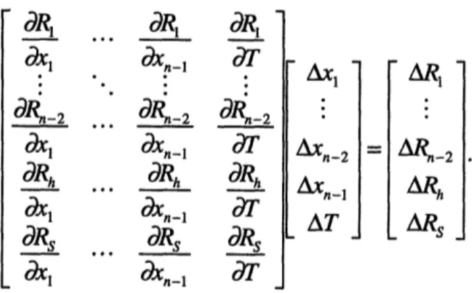
In contrast to a final equilibrium problem, where energy is conserved, in a re-versible process problem, entropy remains constant. Computationally, this means replac-ing the energy conservation equation by a conservation of entropy equation. It is also necessary to specify a final state property for one of the elements in the mesh, in order to dictate the final state of the system. This state property is termed the handle, h. The goal of the process is go from h to hf while keeping the system entropy constant. This results in an extra residual equation in the system. The new set of equations are of the form

n = ~F i ; i = 1,2,...,n - 2 (2.15) j=l n Rs = sJ --Sog (2.16) j=l Rh =h-hf. (2.17)

These equations are solved using the Newton-Raphson method. The linearized equations in matrix form are given by

...

dR1 dx1 0, bl-2

d

1 dRh

d

1 dRs x 1 d·, OXn-l

. dn

Rn-2 Rh dXnil_0es . . . ObXn-l SI dT d'k-2 dT dT -An-2 AXn-I AT AR, ARn-2 ARh ARs (2.18)

The partial derivatives in the stiffness matrix of equation (2.18) are generally derived the same way as the final equilibrium case. The partial derivatives for Rh and R are calcu-lated below. Ra V =h (Ajaj) dxj dV dxj dV dR Ah R h

dT dT

dRS dS = n dSk Vk

dx

1

_

: dVk

dxj

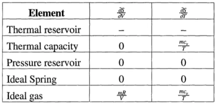
(~j k=l &j k=l dRs n dSk ORs = _=T O

The expressions *, ,

4

and

4

are tabulated below.

h _ _ F V 1 0 p -T 0 1 n 2j k

k(

aj )

Table 2.4: Handle derivatives for Stiffness Matrix

(2.19)

(2.20)

(2.21)

dS dS Element dV as Thermal reservoir - -mcy Thermal capacity 0 - T Pressure reservoir 0 0 Ideal Spring 0 0 Ideal gas m..mR mCT Ideal gasI T

3 Pure Substance Element Modeling

3.1 Overview

The modeling of the pure substance element requires the use of an explicit analyt-ical function of sufficient accuracy. This function is the P - p - T constitutive relation, also known as the equation of state for the substance. Ideally, this equation would be valid for the solid, liquid and vapor phases of the substance. However, the behavior of the properties is so different for the various phases that a common approach is to develop

P- p - T functions valid for each phase or combination of phases of the substance. This

model is very general and represents a system without chemical reactions. The pure sub-stance model is very useful in an ample range of physical situations and thermodynamic applications. It requires additional attention when applying the first and second laws of thermodynamics than is necessary for the ideal gas element. In particular, the possibility of a phase change that accompanies any property change in the pure substance model re-quires evaluation of the substance from charts or tables. For the purpose of developing and implementing an algorithm within the CAT program framework, we consider the case of water as a pure substance. Its phases most frequently found in thermodynamic applications are vapor, liquid-vapor mixture, and liquid.

3.2 Equations for Water Vapor and Liquid Regions

The expressions we will need for this region, as required by the CAT algorithm, are P = P(p,T), U = U(p, T), and S = S(p, T). In this model of water as a pure sub-stance we will adopt the basic constitutive relations from the steam equations as pre-sented in Reynolds, W., Thermodynamic Properties in SI, Stanford University, 1979, which are a slightly modified version of the ones used in Keenan, J., et al., Steam Tables, John Wiley and Sons, 1969. The P - p - T equation is given by:

P=pRT[ l+pQ+p d J (3.1)

where, 7 8

Q =

-. c) ( _ .i

(

.

)

1

Ai

(P

- Pai

)

j=l i=1 = 1000 / T Ta, = 1. 5449121; aj= 2.5, 10

+ e-PA jIpi

_-

9

i=9]

j>l

Pat = 634; Paj =1000, j > 1 E=4.8x10 -3; R= 461.51 J/kg K

and A, is as shown in Table 3.1. Constants for T in K, p in kg/m3 and P in Pa.

In order to find the term ( )let us first define

8 10

Hj(p) = Al(P Paj))i-1_{+ e-EPI Api-9}

i=l ~ i=9

Hj8~p) == i p-j - +10

(p-

)-2_

EeEp XA-pi - 9_{+ e-EPAlo}

dp i=2 i=9 l

=2P = (l-1_

+

d

Hj (p) )i-3 2

H;'(p)

= dp) =

-

1)(i-

2)(p-

Paj) +

dp i=3 i=9

we then find (P)T as follows:

(dQI

d p )T

7

==1 (_aj)j-2 H,(p).

j=l

The energy equation can be written in terms of the specific energy,

U(p, T) = mu(p, T)

(3.7)

(3.8)

where m is the mass and

(3.9) (3.2) (3.3) (3.4) (3.5) Ep Aloj (3.6)

A4.pi

- 9

- 2Ee'

T

f' cO

(T)dT

+

f' P

pi

-T-dp +

dp

uO

T 2

0P -

OT

P

-oo a I~~ C) x 0 x 6 x -X X X 0 tn 00 ·d' o £ 00 co0 0 , ooo x xxo -4 - 0 0~~~~0 0 O O 0 0 0 0 ll In) -0 x x x x ,It N l c cN Cl CO C 'I cqi IT w X X X st O O) 00° -4 - - 0 x x x --on, " Cl 1-I - m 00 M o O X X X X x 000X x x in . 1,0 oo CO - Cl 00 0606 x 0 C Cl x x Cl ON N O O -m C C ,, ,~. 0 o

0 0

,- 4 - 4 - 4 -4 -X X X X X Cl CO ~ 0 0 \,0 It _N I) - 00 CO 00 - 001,0 00 'C N -4 00 'Ct t oll CO 00 N N in N O - 4; - f; Xl X c o t_ O ><

0

x

"

00 cO 00 N -00 00 CO

o

0)

66

-4 . -. X XN 00 0 c- , Co 0~ (Do ,o X X o

~U

00 00 N - o .. C O COF 10 C_ o O -4o o-4 x x X X X Cl

~

N 00 0) CO e 00 0 %n 0 _{i N} 0 CO 0) 0 1,0 in ON - -I - kn I I -

N C t i

- o

N,0

ON 0

- -x x N mn '- CO a)- lfrI Cl C 6 C

o

it -4 x x O 0 N r Ne N 00 c ON oN N- cOi ,_

o-@P)

-pR

1+pQ+pTTQ

d +

2TdQ

dr +P

2<QI a P - d'v dT dp TdT dpT dz

_1000

z dT 2 T

T

p

[

(dPl

P lp+RTQ+RT

fJ

7,

P-[yaTodp

=

o

+ R + pR

lilT

p~L

0

-,

P

I

T (3.11) - T dP ]dp 1p d. P J ,dp = RT2 fd P dQ

dT fOp[ Yr)

- -T

drP-

dI

dT a dT )p -

100pR

dQ-=

I('

V'j)

_ j -

2 +

( -

Vc)(J

- 2)( - aj

)

Hj(p).

/=1 Simplifying, we obtain where, dQ daT P u = cv (T)dT+ 1000pR - + uo P 7

=

,[(j

-2)( -c)(r-

,)

_j

.-

_{3 + (}

_{- r. )-2}

_]H.(p)

j=l To= 273.16; u = 2375020.7 J/kg 6 c (T) = I GT' -i= G1 = 46000 G2 = 1011.249 G3 =0.83893 G4 = -2.19989 x 10- 4 G5 = 2.46619 x 10- 7 G6= -9.7047 x 10-" where, (3.10) (3.12) (3.13) (3.14) (3.15) (3.16) 1[l = -RT 2 dc P dT fo, IdQ

.dpT

fTC (T)dT =G lnT + 6 G i il TOi-i ' 6 Gi T

i-i=2 i=2 -I

=GIlnT+ Gi Ti-'1- 564413.52

i=2 1 -1

u is in J/kg, cv in J/kg.K. The equation for specific entropy is given by

so= 6696.5776

6 Oi T- 2+Gl6

21nTo_2

dt G = -- + G21n T + = i -2 +- TO 2 - To i-2

GoT

T i=3i-2 Toi°

i=3

°

L+ G21n T + Ti-2 -5727.2610 T 2i--PR- 1 l ( )]

d

d

-pTo -- pRT-

-

-dp

dT p dT d VP T dTJ = R

-Q-p

QC

+;Q = pR -PQ+T ) ]

.~I

Q

,

( oo P d (Q p s is in J/kg-K.

The preceding equations will allow us to determine pressure, specific energy and specific entropy as a function of density and temperature. They are valid for the vapor

and liquid phases of water.

(3.17)

s = JdT-Rlnp+f

pR-KJroT where, ( hp

0

+

s

d;. +~o (3.18) (3.19) (3.20)

3.3 Equations for Water Liquid-Vapor Mixture (Saturation)

The expressions needed for this region, as required by the CAT algorithm, are again,

P = P(T), U = U(p,T), and S = S(p,T). The P- T equation is given by:

PPCexP{(Tc /T-)Fa(T-T)]

}

P = P exp (T / T - 1)1_,Fi[a(r -

rp)]

i=1 (3.21) where, Pc = 22.089 MPa; Tc = 647.286 K F1 = -7.4192420 F2 = 2.9721000 x 1071 F3=-1.1552860 x 10-' F5 = 1.0940980 x 10-3 F6 =-4.3999300 x 103 F7 = 2.5206580 x 10-3 F4 = 8.6856350 x 10-3 F8 =-5.2186840 x 104 a=0.01; Tp =338.15 K.

The energy equation is given by

U(p, T) = mu(p, T) = m(uf + XUg)

where,

Uf

= u(pf

,T)

in which the function u(p, T) is as given in equation (3.14), and

pf = pI + Dj(l-

T

l

TC)

l

i=l (3.22) (3.23) (3.24) where, Pc = 317.0 kg/m3 D1 = 3.6711257 D2=-2.8512396 x 101 D3= 2.2265240 x 102 D =-8.8243852 x 102 Ds = 2.0002765 x 103 D6 =-2.6122557 x 103 D7 = 1.8297674 x 103 D =-5.3350520 x 102

V-Vf V-Vf 1/p-1/pf

Vfg Vg -Vf 1 pg-1 / pf

Pg P(Psat,Tsat)

-(3.25)

(3.26)

We have not defined an explicit function for p = p(P, T) as expressed in equation (3.26) and there was not one available. However, pg as a function of T can be computed by us-ing the followus-ing methodology:

1) given the temperature, T, we use equation (3.21) to calculate P,

2) using these two values (T,, Pst) we iterate in equation (3.1) to obtain pg. An iteration scheme such as Newton-Raphson can be used, where

k+l k

Pg =pg

P(pg, Tsat) - Psat

ap(pkkTM) aP

The Newton-Raphson algorithm requires an initial guess, pO. The equation for specific energy in the saturated region is

Ug = u(pg, T)

where, again, the function u(p,T) is as given in equation (3.14). Finally we have

ug =u -uf .

The entropy equation is given by

S(p, T) = ms(p, T) = m(sf + XSfg)

where,

Sf = s(pf,

T)

in which the function s = s(p,T) is as given in equation (3.18). Similarly,

5_{g = s(pg, T)}

where pg is calculated as previously explained.

(3.27)

(3.28)

(3.29)

(3.30)

3.4 Stiffness Matrix Expressions for Water Vapor and Liquid Regions

The derivatives required for the Newton-Raphson stiffness matrix, namely (V)T'

(-)v' rV)T' (v) ,,)v and ()v _{are calculated below, from the equations in}

sec-tion 3.2:

dP

(dP) dp _ m1 (dP) (3.32) YdV)T SP )T dV - V2 dP

dP R 1+

pQ +P2

d +

32

dQ +

(.4d)1

(3.33)

-dPi

=

RT[l+2pQ+p2pJ

+3p

p

)T

p

2 T where,

j2Q

D

T

--

(

_r

)

_-

_'aj) -2_H;'(p).

_(3.34)

T ~~j=1

The other pressure derivative we seek is (p)v, which was already calculated as equation (3.10) (Section 3.2).

The first energy derivative, ( )T' is found as

(dU"A

(duA _A

dp

2

(du

TU ddu _{dp M du}

ZV) = ) =M Z= dV =_ V P (3.35)

)T=

10OjR

dQ

+ Pd

Q

₂₁

(3.36)

d-V T

[Pr

,Vr

-

_{V- J}

=

_{~P r}

We had already calculated ()) in equation (3.13). The second energy derivative is

(dub

=c (T)+ OOOpRd2Q) = c°(T) - pRT2(

dQ)

~TTp where a2 7

(d e :[(J

- 2)(j- 3)(,r

-

c)(

-

arj))

-

4 + 2(j - 2)(r- raj)-3 ]Hi (p)

The first entropy derivative, (v)T, is found as

(dS) =md S) =m(dS) dp

_m 2_{1ds )}

(ds

R 1

L

dTP)] 1 (dTP)

p=

_+Z~

r

_R

=

where )p was calculated in equation (3.10).

The second entropy derivative is

(

=

m)

s

= C0

TC

T - pR (.

3.5 Stiffness Matrix Expressions for Water Liquid-Vapor Mixture (Saturation) The (V)T derivative is found to be equal to zero, since, in this region, P is not a function of V. The second pressure derivative is found as

=P exp

-

)

I

F

a(T

-)]

(3.44)

+aT --1 (i

/i=2) -

1)F[a(T-

Tp)]i 2}. d, dT (3.38) (3.39) (3.40) (3.41) (3.42) (3.43) (dP> tdT at T I . I X - C I F,[a(T - T,)]' T 2 i=1

The first energy derivative, (uV)T is calculated as follows. dUT

uT

5aV T V T where, (Uf + XUfg

dvv

V-V X= f Vfg )T U fg dx (d) 1 O T Vfg and so,

CU

dV T Ufg = Vfg U_{U fg} 11

_Pg

_{- llpf}

The second energy derivative, (-u)v, is found as shown:

(dU) =m(du = m a(uf + Xufg)v

=M d-uf+x dUfg x Ufg dT dT dT

)v

fg where,

=(vvf) d

iJ_ dvf1)

dT fg )dT (vfg)

= (v + x~-Vf)(-

_{=(f +fgf}

C

_v2dT

1

dg dvf

_dT

(I'

_fg

-(v-,,~¥j- 7~¥

x dVfg Vfg dT dvf dT dv 1f 1 dT Vfg dvfg 1 dT Vfg (3.45) (3.46) (3.47) (3.48) (3.49) (3.50) (3.51)

dvf

d_

i

I dpf dT dTpf pf dT

dpf iD,

(-TITC

)i3-1 dT i=P c

(3.52)

(3.53)

Since we do not have an explicit function for g we need to find a numerical approxima-tion to d -. This is given by

where,

dvfg dVg dvf (354)

dT dT dT

dvg vg(T + AT)- g(T) (355

dT AT

We can calculate d- as,

duf uf(T+AT)- Uf (T)

dT AT

where - is as given in equation (3.38). Similarly, for d, we find that

dug ug(T+ AT) - Ug(T)

dT AT dufg dT - dug dT (3.56) (3.57) (3.58) duf dT

The entropy derivatives are calculated in similar fashion,

(3.59)

C-T T-)

d dx

= - (Sf + XSfl)T = Sf9

-Is~

ds

-/

°

₎

_-t

_mM(Sf

_+Xsfg)v

dT

-

dT

d

[ds

V

df

+@~ dx g (3.60)

j=

d~fg +X

(+

x

dT dT dr )vsfg where, dsf Sf (T + AT)- S (T) (3.61) dT AT dSg sg(T+ AT)- sg(T)

(362)

dT

/\T ~~~~~~~~~~(3.62) dT AT dsfg = dsg dsf (3.63) (3.63) dT dT dT

3.6 Behavior of the Pressure Function

The behavior of the P- p - T function (Eq. (3.1)) was studied for the working range of steam (liquid, liquid-vapor and vapor regions). The function is able to describe both liquid and vapor phases, however we are also interested in looking at the behavior of the equation in the saturated steam region for the purposes of developing the CAT algo-rithm equations.

Equation (3.1) was plotted as a continuous function from the liquid phase up to the vapor phase. The intention was to obtain an idea of the accuracy of the function com-pared to the numbers in the Steam Tables, and to get a sense of the sensitivity of the function, especially in the liquid phase. We were also interested in the behavior of the function in the vicinity of the critical state.

Figure 3.1 gives an idea of the proportions of the P- p - T surface by showing the relative sizes of the liquid, liquid-vapor, vapor, and gas regions. Figure 3.2 zooms in the

P -p - T plot to show the liquid region and part of the liquid-vapor region. Notice that

some isotherms actually cross the specific volume axis to go into the negative pressure region before coming back and fall in place right at the line of saturated vapor states. Other isotherms cross the liquid region twice, going down and then coming back up.

This behavior has a negative effect in the performance of the Newton-Raphson iteration algorithm.

Figure 3.3 shows the behavior of the function in the vapor, gas and part of the liquid-vapor regions. The isotherms are smoother and less sensitive to changes in spe-cific volume than the isotherms in the liquid region. This part of the P- p - T surface is more amicable to the Newton-Raphson algorithm.

= so W/ W) in cs C - - - - N M0 m t m m m r- t II- II kn k It It

a

N m t H 'I cl, 11 11 11 1 1 1 CIO -q Fo E ' 0 C= 0 o0 0 0 0 0 0 0 0 ₀ 0 ₀ 0₀ 0 0 0 0 0 0 CD CD CD CD CD CD CD CD CD CD CD o o CD o or o 0 0 0 0 0 0 0 0 0 0 0 0 0 0 0 0 0 0 0 0 0 0 0 0 0 0 0 0 0 0 (ed) d

0 ~ ~ 9 ON o. " o o

o

_ °~~~

9

-r

0

_

~~o

O~~ o. ~~~~~~~~~~~cj O Cl

~ ~

L 0. 0 o 6 ~ ~~ ~ ~ ~ ~ ~ ~ . o C~S

.,~~~~~

~-.

O xOl ON_0Eo 0l 0 0 0) 0 0D 0 0 0 0D CD 0 0 D CD O 0 O O O O O O O 0 O O O O O O O O O O 0 0 0 0 0 0 0 0 0 0 0 n ' ( N 0 ' ( N 0 N 0 '(N 0 ' I N (d)

d

U I II I I = IC tnI c $. t- 11 n tn -t tI B n F- E c

0

0

0

~

~~ ~~0

0 0

0)

0) 0 0) 0 0) 0 0 0 0 0 0 0 0) (ed) i 8 8

(da)

d

8 8 °~~~~~~ 00 o - - - - cq 00 - l . 00t- II kn II I '-6 t It

a

0H et W) cn; E HH E 00 6

6

$z 0o bb 0 a) . 0 qd Ia 0 ,CI 0 O 0 u c) un O O rn_. ul 6 cle C) ci 6 6 IC 140 o. o 0 0 0 C)

4 Introduction

4.1 cT as the Development Language

The cT programming language provides end-user programmability for creating modern graphics-oriented and multimedia programs, with portability across the most popular computer operating systems; Macintosh, Microsoft Windows (DOS), and UNIX's X-Windows. cT has the mathematical capabilities of algorithmic languages such as C but also offers easy control of modern user-interface features such as graphics, mouse clicks and drags, pull-down menus, rich text, color images, and digital video.

Like C, cT offers the advantages of a modular programming language. cT pro-grams are divided into subdivisions called "units". Each unit has a unique name by which it is referenced. A unit may use variables which are local to that unit. Local vari-ables are defined and are valid within each unit. If no local varivari-ables are used, all global variables are automatically available to the unit. The unit can also use both local and global variables. Modularity of the CAT program is useful to separate main algorithmic units, where the computational part of CAT is handled, from other support units, such as graphic input/output routines.

cT also offers dynamic memory allocation, in the form of dynamic arrays. In certain software applications the size of an array of variables may not be known a priori. This is the case in CAT where the size of some arrays, especially those related to the number of elements in a mesh, is not know initially. cT provides computer commands that lengthen or shorten dynamic arrays, for an efficient memory management.

The cT programming environment was developed in the Center for Design of Educational Computing at Carnegie Mellon University, in 1989. The CAT source code for steam modeling presented in this thesis was written in cT version 2.0. Currently, cT is available on MIT's Project Athena by typing:

add at; cT

5 The CAT Software

5.1 Organization

The CAT algorithm was programmed as an interactive computer program using the cT language. The resulting computer software is designed to help the user assemble a given thermodynamic problem as a mesh of elements, using the approach presented in Part 1, and perform a simulation to obtain a numerical solution. All of this is done through a user-friendly graphical interface consisting of windows, icons, and pull-down menus which simplifies the use of the program. The graphical interface brings the soft-ware up to the modem computer standard, which users have now come to expect.

The cT CAT source code (CAT.t) is included in magnetic media (3.5-inch floppy disk) with this thesis. The units dealing with the steam element, product of this research, are presented in Part 3 of this thesis. The CAT.t source code is divided in six major areas,

these are:

1) mesh creation

2) element property input routines 3) computational algorithm 4) solution presentation

5) element constitutive relations and derivatives database

6) graphical interface support routines.

Their functionality is described in the following sections.

5.2 Mesh Creation

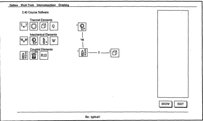
The initial CAT screen (refer to Figure 5.1) is divided in several areas. The left hand side of the screen contains the full library of modeling elements available in CAT, displayed as icons. The user chooses from any of them by simply clicking and dragging the desired element to the work area. The work area, is the empty middle section of the screen. To connect the elements with mechanical or thermal interconnections, the user clicks on the "Interconnections" pull-down menu from the menu bar to choose the desired type of connection. The user then clicks on the first element and drags the cursor to the second element to connect the two. The menu bar at the top of the screen offers various

other choices, such as saving or retrieving a mesh file, changing values, deleting icons, and other useful functions for generating and simulating the mesh. The status line is

lo-cated at the bottom of the screen and is used to prompt and aid the user to enter data, and

display error messages. Finally, the area in the right hand side of the screen is the data entry window. This is where the user initializes the mesh by entering the initial proper-ties of the elements and interconnections.

Figure 5.1: CAT initial screen

Creation of the mesh consists of placing the desired element icons on the work area, and connect them with mechanical or thermal interconnections. While this is hap-pening, the program checks to prevent the user from creating an unsolvable mesh. For instance, a mesh can have no more than one mechanical matching element. The program also prevents the user from connecting incompatible elements, such as thermally

connect-ing an ideal sprconnect-ing to a thermal reservoir. Opdons Mesh Tools Intercomecdons Graphing

2.40 Course Softare Thermal Elements Mechanical Elements Coupled Elements F 1 ~F~ 12I SHOW |EXIT file: typicall 1 F67 I -UPI I IM I 11 ORS I - T 151

-5.3 Input Routines

At the beginning of each run of CAT, the global variables (valid for all units) are defined and initialized in the Initial Entry Unit (IEU). The IEU refers to those commands which appear before the first unit command. After the IEU is finished, execution pro-ceeds to the first unit in the program. The IEU is the appropriate place to define all the variables that are going to be used in all or most of the program units.

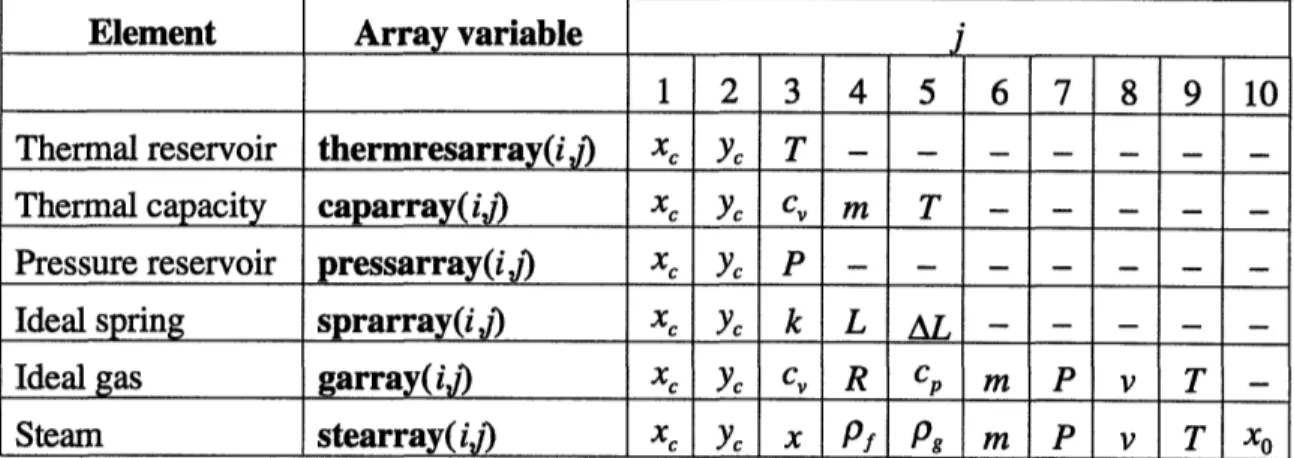
The handling and storage of the element properties is performed in arrays that are defined for each element type available in CAT. The element array variables used in the program and their storage organization are shown in Table 5.1.

Table 5.1: Element array organization

The first index in the array, i, denotes the element sequence number in the mesh. The second index, j, denotes the local state parameter. For example, thermresarray(2,3) is the temperature of thermal reservoir number two. Note that for all elements, the first two array values are the (x,y) screen position coordinates of the element in the mesh. These arrays house the initial values of the properties, and remain constant during the algorithm execution. The only exception is the steam element array, stearray(ij). During execu-tion of the algorithm, it is necessary to know the steam quality, so as to determine the steam state (liquid, liquid-vapor mixture, or vapor). Therefore, at every step of the itera-tion algorithm, the values of quality, x, saturated liquid density, Pf, and saturated vapor density pg, are updated and checked for possible phase change. The initial value of quality is stored in stearray(i,10).

Element Array variable

-_1

2 3 4 5 6 7 8 9 10

Thermal reservoir thermresarray(ij) Xc Yc T - - - -Thermal capacity caparray(ij) xc Yc cv, m T . . .

Pressure reservoir pressarray(ij) XC Yc P _ _ _

Ideal spring sprarray(ij) xc Yc k L AL … … _

Ideal gas garray(ij) xc Yc cv, R cp m P v T

Once the mesh has been created, the elements and interconnections must be ini-tialized. To do this the user clicks on the icon to open up the data entry window. The user then enters the properties required to define the element's initial state. These proper-ties are listed in Table 5.1. The only interconnection type that requires initializing is the mechanical interconnection. The boundary area associated with the mechanical intercon-nection must be entered to initialize it.

The program also verifies whether negative values for properties such as pressure or temperature were entered. In that case the user is prompted to re-enter new values.

5.4 Computational Algorithm

The mesh is solved with the Newton-Raphson algorithm as described in Section 2.5. This is carried out in the unit numerical of the CAT source code. The flowchart shown in Figure 5.2 describes the solution process used by CAT. Subroutines used by the unit numerical are included in parentheses at some of the flowchart steps. At the start of the unit, there is a first check to determine whether all elements and interconnections have been initialized. The program checks in the variable track(ij) which among other functions, keeps record of which elements have been initialized. In the unit makemats, the matrices used to setup the Newton-Raphson system equations are setup. This unit also sets the initial guess for the displacement and temperature vector, xvector(ij). The initial guess for the displacements is zero, and the initial guess for temperature is taken from the initial Ideal Gas or Steam Element temperature. If there is a thermal reservoir in the mesh, the initial guess is set to the reservoir temperature.

The residuals are calculated for the initial conditions, and then checked to see whether they are still larger than the specified tolerance (0.00003, arbitrarily set). Once the residuals are less than the tolerance, equilibrium is reached and the problem is solved. Otherwise, the program uses the Newton-Raphson algorithm to estimate a better solution set. At every step of the iteration, the program performs two checks to make sure it is converging. In the first check the program verifies the updated properties; if the volume or temperature of any element becomes negative, the program will reduce the change vector (cvector) in half and calculate a new solution vector. This is done in case the al-gorithm overshoots the solution vector. In the second check, the program calculates the normal of the vector containing the force and energy balance equations (vector function).

At equilibrium this vector should be a column of zeros. The program compares the new normal with the old normal from the previous iteration. If the new normal is smaller than the old normal, then iteration is proceeding in the right direction and the program resumes the iteration loop. Otherwise, the change vector is cut in half, and a new solution vector is calculated. If the change vector is cut in half for 13 times (arbitrary number), it is as-sumed that the equation system is just not converging, and execution of the program halts with an error message.

As a way of diagnosing the progress of the Newton-Raphson iteration, the pro-gram displays the word "Calculating" in the status line at the beginning of the numerical simulation. Then, for every successful iteration a period (".") is printed in the status line. For each time the change vector has to be halved because a negative temperature or vol-ume was calculated, the program prints a question mark ("?"). Finally, every time the change vector is adjusted because the new norm is larger than the old norm, an exclama-tion point ("!") is printed in the status line. The symbols get printed next to each other.

Yes

Calculate initial residuals

(unit makeinitial) No quilibrium reached old norm kenorm) j=0 Yes Yes

top and print error are OK. :w residuals efunction) new norm kenorm)

I

0

rmS

tom II Il l l r

5.5 Solution Presentation

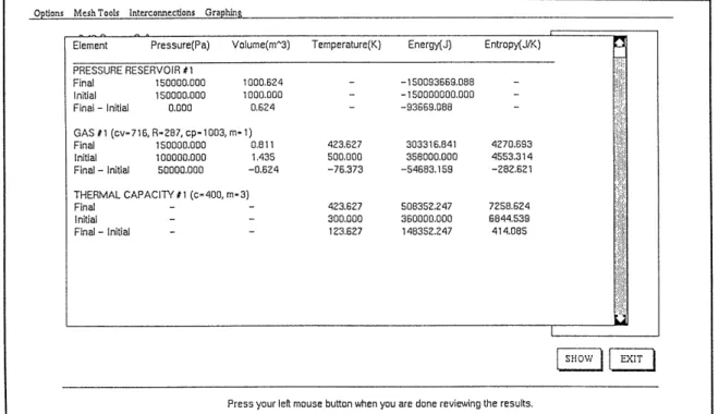
After a successful run, the solution is presented in tabular form. A pop-up win-dow appears on the screen listing all elements present in the mesh, along with their initial and final state properties. The properties change from initial to final is also calculated. A typical results window is presented in Figure 5.3. The properties listed for each element are pressure, volume, temperature, energy and entropy. S.I. units are used throughout the program.

Figure 5.3: CAT results screen

For the case of reversible problems, the user has the option of plotting the re-versible process in terms of the main properties. Prior to starting the numerical simula-tion, the user is asked to specify the number of intermediate states that will be used to create the plots. After a successful run, the user has the choice of plotting pressure vs. volume, pressure vs. temperature, and volume vs. temperature for any of the gases (Ideal Gas or Steam Element) in the mesh.

Element Pressure(Pa) Volume(mt3) Temperature(K) Energy(J) Entropy(J/K) PRESSURE RESERVOIR #1 Final 150000.000 1000.624 - -150093669.088 -Initial 150000.000 1000.000 - -150000000.000 -Final - Initial 0.000 0.624 - -93669.088 -GAS #1 (cv=716, R287, cp=1003, m= 1) Final 150000.000 0.811 423.627 303316.841 4270.693 Initial 100000.000 1.435 500.000 358000.000 4553.314 Final - Initial 50000.000 -0.6Z24 -76.373 -54683.159 -282.621 THERMAL CAPACITY 11 (c=400, m-3) Final - - 423.627 508352.247 7258.624 Initial - - 300.000 360000.000 6844.539 Final - Initial - - 123.627 148352.247 414.085

Options Mesh Tools Interconnections Graphing

Press your left mouse button when you are done reviewing the results.

- - - I

I

5.6 Relations Database

All constitutive relations listed in Table 2.1, and derivatives listed in Tables 2.3, 2.4, and 2.5 are programmed in CAT as functions. These functions are called as needed by the main numerical algorithm. The constitutive relations from Table 2.1 of pressure, energy, and entropy are programmed in the unit makefunction of the CAT source code. This unit contains the constitutive relations of all elements available in CAT. However, the constitutive relations of the steam element are programmed separately, since they are referenced from other units as well.

The derivatives required for the Stiffness matrix in the Newton-Raphson algo-rithm are also programmed in the CAT source code. The units drdx, drdt, drEdx, drEdt, dhdx, dhdt, drSdx, and drSdt correspond to the derivatives R R RE, dh

A 9S ds ~ ~ ~ ~ ~ ~ ~ ~~~~~~x d'd' T x , "s and dT, respectively. Within each unit the derivative is calculated for each of CAT's elements.

5.7 Graphical Interface Routines

One of the key features of the cT language is its ease of programming graphic tools for user-friendly displays. CAT makes use of cT's graphic commands in setting up the screen display and handling the icons for mesh creation. Various units in the CAT program take care of the graphical management of the screen. The main units are:

unit display creates screen display and menus

unit buttons draws "SHOW" and "EXIT" screen buttons unit boxes draws palette of element icons

unit drag allows dragging of element icons around the screen unit clean clears status line from text

unit finder tracks mouse movement of screen cursor

6 Steam Element Software Development

6.1 Input Routine

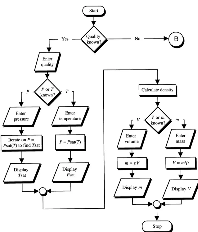
When initializing any element in CAT, the user should be able to enter the mini-mum number of properties that will precisely define the state of the element. This is true for the Ideal gas element, where the user needs to enter just three of the four properties from the equation of state (P, m, V, or 7) to completely define the state of the gas. The program takes care of calculating the fourth property from the other three. This feature is also desirable in the Steam element. However, steam has an additional property that the Ideal element lacks; quality. Since quality tells use whether we are dealing with a multi-phase substance or a single multi-phase substance, it is helpful to ask the user for the value of this property first. The steam quality dictates what set of constitutive relations is appro-priate to use. Recall that the common approach in modeling a pure substance is to define constitutive relations valid for a specific phase (or combination of phases) of the sub-stance. The user may or may not know the initial steam quality, and the input algorithm should be able to handle both instances.

6.1.1 Known Quality

When the quality of steam is known, the applicable set of equations is as given in section 3.3, valid for the steam saturated region. The user can then specify either the sat-uration temperature or satsat-uration pressure for the steam. If the satsat-uration temperature is specified, the value is simply plugged in equation (3.21) to obtain the saturation pressure. If the saturation pressure is specified, the program iterates in equation (3.21) to obtain the corresponding temperature. This is done using a Newton-Raphson algorithm,

T7k+l = Tsk _{-a Tat} at _d[L(6.1Psat -P6.1) (t)

dT

The initial guess, Tt, required in the Newton-Raphson iteration is supplied by a function that approximates the unavailable function Tat = T(P). Choosing several equally-spaced

(Tat, Pat) points we came up with the function

which is simply used to obtain a better initial guess for the Newton-Raphson iteration, thereby minimizing computation time.

Once the saturation temperature and pressure have been specified, the user is given the option of entering either the steam mass or volume. At this point, the density of the steam has already been calculated as

p 1 (6.3)

j+x(9

The mass or volume can then be calculated from m = pV. The properties that the user

does not enter are calculated and displayed by the program.

6.1.2 Unknown Quality

The user may skip entering a value for the initial quality. When this happens there are no assumptions made about the state of the steam. Only after the user has en-tered some of the known properties, the program can determine the specific state of the steam. After skipping entering the initial quality value, the user is then asked to enter three of the four steam properties, m, P, V, and T. All possible combinations are studied and discussed below.

* Known P, V, m

To calculate the missing property, temperature, the program first needs to know whether to use the P -p - T equation (Eq. (3.1)) valid for liquid and vapor states, or to use the

P- T equation (Eq. (3.21)) for saturated steam. From the given pressure, the program

calculates the saturation temperature, Tat using equation (6.1). The saturated liquid den-sity and saturated vapor denden-sity are calculated for this temperature. The denden-sity of the fluid is calculated as p = m / V. If the density is less than Pf and larger than pg, then the steam is saturated and the calculated Tat is the temperature we are seeking. Otherwise, the temperature is calculated from

Tk+l = Tk - P(p, Tk) P (6.4)

dP(p,Tk) dT