HAL Id: hal-02489682
https://hal.archives-ouvertes.fr/hal-02489682
Submitted on 10 Nov 2020
HAL is a multi-disciplinary open access
archive for the deposit and dissemination of
sci-entific research documents, whether they are
pub-lished or not. The documents may come from
teaching and research institutions in France or
abroad, or from public or private research centers.
L’archive ouverte pluridisciplinaire HAL, est
destinée au dépôt et à la diffusion de documents
scientifiques de niveau recherche, publiés ou non,
émanant des établissements d’enseignement et de
recherche français ou étrangers, des laboratoires
publics ou privés.
Public Domain
CoMPARA: Collaborative Modeling Project for
Androgen Receptor Activity
Kamel Mansouri, Nicole Kleinstreuer, Ahmed Abdelaziz, Domenico Alberga,
Vinicius Alves, Patrik Andersson, Carolina Andrade, Fang Bai, Ilya Balabin,
Davide Ballabio, et al.
To cite this version:
Kamel Mansouri, Nicole Kleinstreuer, Ahmed Abdelaziz, Domenico Alberga, Vinicius Alves, et
al.. CoMPARA: Collaborative Modeling Project for Androgen Receptor Activity. Environmental
Health Perspectives, National Institute of Environmental Health Sciences, 2020, 128 (2), pp.027002.
�10.1289/EHP5580�. �hal-02489682�
CoMPARA: Collaborative Modeling Project for Androgen Receptor Activity
Kamel Mansouri,1,2,3Nicole Kleinstreuer,4Ahmed M. Abdelaziz,5Domenico Alberga,6Vinicius M. Alves,7,8Patrik L. Andersson,9 Carolina H. Andrade,7Fang Bai,10Ilya Balabin,11Davide Ballabio,12Emilio Benfenati,14 Barun Bhhatarai,15Scott Boyer,16 Jingwen Chen,17Viviana Consonni,12 Sherif Farag,8Denis Fourches,18Alfonso T. García-Sosa,19Paola Gramatica,15 Francesca Grisoni,12 Chris M. Grulke,1Huixiao Hong,20Dragos Horvath,21Xin Hu,22Ruili Huang,22Nina Jeliazkova,23 Jiazhong Li,10Xuehua Li,17Huanxiang Liu,10Serena Manganelli,14*Giuseppe F. Mangiatordi,6** Uko Maran,19 Gilles Marcou,21Todd Martin,24Eugene Muratov,8Dac-Trung Nguyen,22Orazio Nicolotti,6Nikolai G. Nikolov,13 Ulf Norinder,16Ester Papa,15Michel Petitjean,25Geven Piir,19 Pavel Pogodin,26Vladimir Poroikov,26 Xianliang Qiao,17 Ann M. Richard,1Alessandra Roncaglioni,14Patricia Ruiz,27Chetan Rupakheti,24,28Sugunadevi Sakkiah,20
Alessandro Sangion,15Karl-Werner Schramm,5Chandrabose Selvaraj,20 Imran Shah,1Sulev Sild,19Lixia Sun,29 Olivier Taboureau,25Yun Tang,29Igor V. Tetko,30,31Roberto Todeschini,12Weida Tong,20Daniela Trisciuzzi,6 Alexander Tropsha,8George Van Den Driessche,18Alexandre Varnek,21 Zhongyu Wang,17Eva B. Wedebye,13 Antony J. Williams,1Hongbin Xie,17Alexey V. Zakharov,22Ziye Zheng,9and Richard S. Judson1
1National Center for Computational Toxicology, Office of Research and Development, U.S. Environmental Protection Agency (U.S. EPA), Research Triangle
Park, North Carolina, USA
2ScitoVation LLC, Research Triangle Park, North Carolina, USA 3
Integrated Laboratory Systems, Inc., Morrisville, North Carolina, USA
4National Toxicology Program Interagency Center for the Evaluation of Alternative Toxicological Methods (NICEATM), National Institute of Environmental
Health Sciences, Research Triangle Park, North Carolina, USA
5Technische Universität München, Wissenschaftszentrum Weihenstephan für Ernährung, Landnutzung und Umwelt, Department für Biowissenschaftliche
Grundlagen, Weihenstephaner Steig 23, 85350 Freising, Germany
6Department of Pharmacy-Drug Sciences, University of Bari, Bari, Italy 7
Laboratory for Molecular Modeling and Drug Design, Faculty of Pharmacy, Federal University of Goiás, Goiânia, Brazil
8Laboratory for Molecular Modeling, University of North Carolina at Chapel Hill, Chapel Hill, North Carolina, USA 9
Chemistry Department, Umeå University, Umeå, Sweden
10School of Pharmacy, Lanzhou University, China 11
Information Systems & Global Solutions (IS&GS), Lockheed Martin, USA
12Milano Chemometrics and QSAR Research Group, Department of Earth and Environmental Sciences, University of Milano-Bicocca, Milan, Italy 13
Division of Risk Assessment and Nutrition, National Food Institute, Technical University of Denmark, Copenhagen, Denmark
14Istituto di Ricerche Farmacologiche“Mario Negri”, IRCCS, Milan, Italy 15
QSAR Research Unit in Environmental Chemistry and Ecotoxicology, Department of Theoretical and Applied Sciences, University of Insubria, Varese, Italy
16Swedish Toxicology Sciences Research Center, Karolinska Institutet, Södertälje, Sweden 17
School of Environmental Science and Technology, Dalian University of Technology, Dalian, China
18Department of Chemistry, Bioinformatics Research Center, North Carolina State University, Raleigh, North Carolina, USA 19
Institute of Chemistry, University of Tartu, Tartu, Estonia
20Division of Bioinformatics and Biostatistics, National Center for Toxicology Research, U.S. Food and Drug Administration, Jefferson, Arkansas, USA 21
Laboratoire de Chémoinformatique—UMR7140, University of Strasbourg/CNRS, Strasbourg, France
22National Center for Advancing Translational Sciences, National Institutes of Health, Rockville, Maryland, USA 23
IdeaConsult, Ltd., Sofia, Bulgaria
24National Risk Management Research Laboratory, U.S. EPA, Cincinnati, Ohio, USA 25
Computational Modeling of Protein-Ligand Interactions (CMPLI)–INSERM UMR 8251, INSERM ERL U1133, Functional and Adaptative Biology (BFA), Universite de Paris, Paris, France
26
Institute of Biomedical Chemistry IBMC, 10 Building 8, Pogodinskaya st., Moscow 119121, Russia
27Computational Toxicology and Methods Development Laboratory, Division of Toxicology and Human Health Sciences, Agency for Toxic Substances and
Disease Registry, Centers for Disease Control and Prevention, Atlanta, Georgia, USA
28Department of Biochemistry and Molecular Biophysics, University of Chicago, Chicago, Illinois, USA 29
Department of Pharmaceutical Sciences, School of Pharmacy, East China University of Science and Technology, Shanghai, China
30BIGCHEM GmbH, Neuherberg, Germany 31
Helmholtz Zentrum Muenchen– German Research Center for Environmental Health (GmbH), Neuherberg, Germany
BACKGROUND:Endocrine disrupting chemicals (EDCs) are xenobiotics that mimic the interaction of natural hormones and alter synthesis, transport, or met-abolic pathways. The prospect of EDCs causing adverse health effects in humans and wildlife has led to the development of scientific and regulatory approaches for evaluating bioactivity. This need is being addressed using high-throughput screening (HTS)in vitro approaches and computational modeling.
OBJECTIVES:In support of the Endocrine Disruptor Screening Program, the U.S. Environmental Protection Agency (EPA) led two worldwide consor-tiums to virtually screen chemicals for their potential estrogenic and androgenic activities. Here, we describe the Collaborative Modeling Project for Androgen Receptor Activity (CoMPARA) efforts, which follows the steps of the Collaborative Estrogen Receptor Activity Prediction Project (CERAPP).
Address correspondence to Richard Judson, 109 T.W. Alexander Dr., Research Triangle Park, NC, 27711 USA. Telephone: (919) 541-3085. Email:judson. [email protected] Kamel Mansouri, 601 Keystone Dr., Morrisville, NC 27650, USA. Telephone: (919) 281-1110 ext. 240. Email:[email protected]
Supplemental Material is available online (https://doi.org/10.1289/EHP5580).
*Current address: Serena Manganelli, Chemical Food Safety Group, Nestlé
Research, Lausanne, Switzerland.
**Current address: Istituto di Cristallographia, Consiglio Nazionale delle
Richerche, Via G. Amendola 122/O, 70126 Bari, Italy.
The authors declare they have no actual or potential competingfinancial interests.
Received 6 May 2019; Revised 27 November 2019; Accepted 5 December 2019; Published 7 February 2020.
Note to readers with disabilities:EHP strives to ensure that all journal content is accessible to all readers. However, somefigures and Supplemental Material published inEHP articles may not conform to508 standardsdue to the complexity of the information being presented. If you need assistance accessing journal content, please [email protected]. Our staff will work with you to assess and meet your accessibility needs within 3 working days.
A Section 508–conformant HTML version of this article is available athttps://doi.org/10.1289/EHP5580.
Research
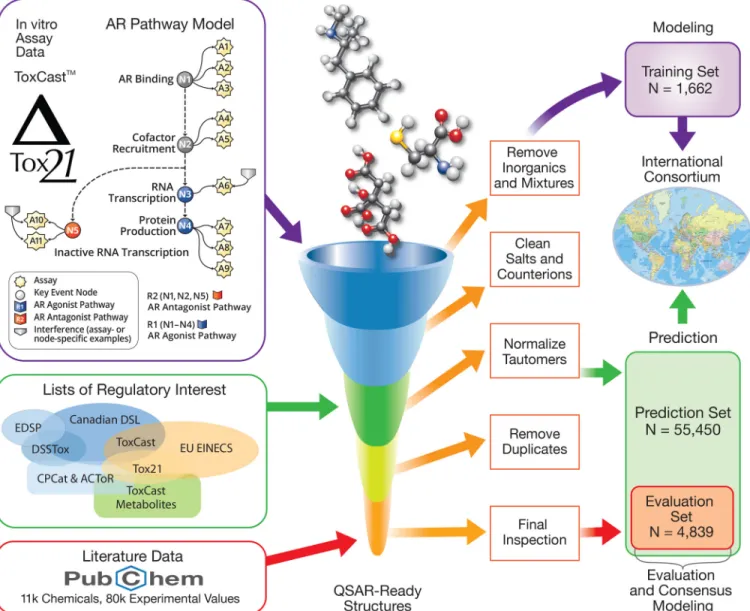
METHODS:The CoMPARA list of screened chemicals built on CERAPP’s list of 32,464 chemicals to include additional chemicals of interest, as well as simulated ToxCast™ metabolites, totaling 55,450 chemical structures. Computational toxicology scientists from 25 international groups contrib-uted 91 predictive models for binding, agonist, and antagonist activity predictions. Models were underpinned by a common training set of 1,746 chemicals compiled from a combined data set of 11 ToxCast™/Tox21 HTS in vitro assays.
RESULTS:The resulting models were evaluated using curated literature data extracted from different sources. To overcome the limitations of single-model approaches, CoMPARA predictions were combined into consensus single-models that provided averaged predictive accuracy of approximately 80% for the evaluation set.
DISCUSSION:The strengths and limitations of the consensus predictions were discussed with example chemicals; then, the models were implemented into the free and open-source OPERA application to enable screening of new chemicals with a defined applicability domain and accuracy assessment. This implementation was used to screen the entire EPA DSSTox database of∼ 875,000 chemicals, and their predicted AR activities have been made available on the EPA CompTox Chemicals dashboard and National Toxicology Program’s Integrated Chemical Environment.https://doi.org/10.1289/EHP5580
Introduction
Humans are exposed to an increasingly high number of natural and synthetic chemical substances (Dionisio et al. 2015;Egeghy et al. 2012;Judson et al. 2009). These exogenous chemicals may have the potential to cause adverse health effects to humans and ecological species (Gray et al. 1997;Safe 1997). The endocrine system regulates a fragile hormonal equilibrium, which might be altered by chemicals that interfere with hormone signaling, e.g., by interacting with its different receptors. Over the last few deca-des, endocrine-disrupting chemicals (EDCs) have been linked to a large number of health issues, including neurological, develop-mental, reproductive, cardiovascular, metabolic, and immune sys-tem disorders (Colborn et al. 1993;Davis et al. 1993; Diamanti-Kandarakis et al. 2009; European Environment Agency 2012;
Martin et al. 2010; Skakkebaek et al. 2011; WHO 2013). The estrogen receptors (ER) and androgen receptors (AR) are among the most studied targets, with a variety ofin silico (Bolger et al. 1998;Judson et al. 2015;Waller et al. 1996),in vitro (Chang et al. 2015;Fang et al. 2000;Rotroff et al. 2010;Shanle and Xu 2011;
Soto et al. 1998), andin vivo (Kleinstreuer et al. 2015;Mueller and Korach 2001;U.S. EPA 2011) EDC screening assays available.
The Endocrine Disruptor Screening Program (EDSP) of the U.S. Environmental Protection Agency (EPA) is one of the larg-est efforts to screen chemicals for endocrine-disrupting potential (U.S. EPA 2014b;U.S. EPA-OCSPP 2014,2015). However, the time and cost to screen the approximately 10,000 chemicals required by EDSP through the entire battery of ToxCast™ endo-crine disruptor assays, estimated at ∼ $1 million USD per chemi-cal, is untenable (HSIA 2009;U.S. EPA 2013,2015). The EDSP has begun to address this resource issue by usingin vitro high-throughput screening (HTS) assays included in the EPA’s ToxCast™ program (Dix et al. 2007;Judson et al. 2014;Kavlock et al. 2012) and the interagency Tox21 collaboration (Tice et al. 2013) involving the EPA, the U.S. Food and Drug Administration (FDA), the National Institutes of Health (NIH), and the National Toxicology Program (NTP). These two programs include assays that measure multiple steps of the ER and AR signaling pathways following the typical nuclear receptor activation process (Judson et al. 2018). Note that the ToxCast™ program also includes a ster-oidogenesis assay in the H295R cell line, measuring perturbations levels of multiple hormones, including testosterone (Haggard et al. 2018;Karmaus et al. 2016). However, the current work does not use this information.
In vitro HTS assays are faster and more cost-effective than traditionalin vivo toxicity testing, and they avoid the ethical con-cerns associated with animal tests. However, no single assay is currently sufficient (due to lack of accuracy, cytotoxicity, solubil-ity issues, etc.) to screen all classes of chemicals for a given mo-lecular target and activity mode (e.g., agonist or antagonist) for an accurate evaluation of potential harm to human health and the environment (Judson et al. 2015, 2018). Therefore, it has been necessary to develop batteries of assays covering various aspects
and steps of the ER and AR pathway signaling processes, which increases the time and costs that are necessary to run and analyze the data. Also, such assays are not applicable to chemicals that are still in the molecular development and optimization phases. Thus, a prioritization of existing chemicals and a virtual screen-ing of new ones bescreen-ing designed are necessary steps to provide knowledge about chemicals with little or no known experimental data (Judson et al. 2018). With the recent technological advances in computational resources and machine learning algorithms, in silico approaches, such as quantitative structure–activity relation-ships (QSARs), are particularly appealing as fast and economical alternatives for their ability to accurately predict toxicologically relevant end points (Dearden et al. 2009; Worth et al. 2005). These methods are based on the congenericity principle, which is the assumption that similar structures are associated with similar biological activity (Hansch and Fujita 1964).
The use of computational methods to screen and prioritize chemicals for endocrine activity has been already initiated at the EPA’s National Center for Computational Toxicology (NCCT), the EPA Office of Science Coordination and Policy, and the NTP Interagency Center for Evaluation of Alternative Toxicological Methods (NICEATM), with a special focus on ER and AR. Starting with ER, a total of 18 ToxCast™ and Tox21 in vitro assays targeting the main estrogen-signaling steps (three cell-free radioligand bind-ing assays; six dimerization assays usbind-ing both ERa and ERb; two DNA binding assays; two RNA transcription assays; two agonist-mode protein expression assays; two antagonist-agonist-mode protein expression assays; and one cell proliferation assay) were run on a library of 1,855 ToxCast™ chemicals (Richard et al. 2016). Then, a mathematical pathway model combined the results into a unique area under the curve (AUC) score [0–1] overcoming the limitations of single assays (assay interference and cytotoxicity) as an estimate of ER pathway activity (Judson et al. 2015). Thesein vitro model scores were then used by a consortium of 40 scientists from 17 inter-national research groups, coordinated by NCCT, in the framework of the Collaborative Estrogen Receptor Activity Prediction Project (CERAPP) (Mansouri et al. 2016a) to develop models for ER bind-ing, agonist, and antagonist activity. A total of 48 QSAR and dock-ing predictive models were developed, which were evaluated usdock-ing an external set from the literature and subsequently combined into consensus models. The consensus models were then used to virtu-ally screen a library of 32,464 unique chemical structures compiled from different lists of interest to the EPA, which identified approxi-mately 4,000 chemicals with evidence of ER activity (Mansouri et al. 2016a). CERAPP demonstrated the possibility of screening large lists of environmentally relevant chemicals in a fast and accu-rate way by combining multiple modeling approaches to overcome the limitations of single models (Mansouri et al. 2016a). In addition to the collected data and the screened list of chemicals, this project also provided a successful collaboration example to follow for using large amounts of high-quality data in model-fitting and rigorous pro-cedures for the development, validation, and use of efficient and accurate methods to predict human or environmental toxicity while
reducing animal testing. Its workflows are now being applied to other collaborative modeling projects for different toxicological end points such as acute oral systemic toxicity (Kleinstreuer et al. 2018b).
Here, we describe a modeling project that aimed to virtually screen chemicals for their potential AR activity. The template pro-cess established by CERAPP was adopted to tackle the AR model-ing project. First, a multiassay AR pathway model was developed based on the results of 11 assays covering the androgen signaling pathway and combining thein vitro results into an AUC score rep-resenting the whole AR activity to mimic the in vivo results (Kleinstreuer et al. 2017). These assays were run on the same initial library of 1,855 ToxCast™ chemicals that the ER assays were run on, and the developed pathway model was validated using refer-ence chemicals with known in vitro results from the literature (Kleinstreuer et al. 2017) and further compared with a set of chemi-cals with reproducible results in vivo (Browne et al. 2018;
Kleinstreuer et al. 2018a). Note that the goal of this project is to predict in vitro AR activity. There is significant discrepancy between in vitro AR activity and the results of the in vivo Hershberger assay, especially for antagonist mode. However, as demonstrated by Kleinstreuer et al. (Kleinstreuer et al. 2018a),
most of these discrepancies are due to thein vivo activity occurring at internal concentrations well above the upper limit of testing in thein vitro assays (100 lM). The resulting AR pathway activity AUC scores were used as a training set in a large AR modeling con-sortium called the Collaborative Modeling Project for Androgen Receptor (CoMPARA). Collaborators from 25 international research groups (Supplemental Material S1) contributed a total of 91 qualita-tive and quantitaqualita-tive predicqualita-tive QSAR models for binding, agonist, and antagonist AR activities. The total list of chemicals that CoMPARA participants screened using their models comprised 55,450 chemical structures, including CERAPP chemicals and ToxCast™-generated metabolites (Leonard et al. 2018;Pinto et al. 2016). These predictions were evaluated using curated literature data sets and then combined into binding, agonist, and antagonist consen-sus models. Both CERAPP and CoMPARA projects were collabora-tions between the participants, aiming to build the best collective consensus rather than competing for the best single model. We also describe the procedure of extending CERAPP and CoMPARA con-sensus models beyond their original lists that was used in the screen-ing of the entire EPA DSSTox database (https://comptox.epa.gov/ dashboard;Grulke et al. 2019) and other chemicals of interest that are structurally similar to the initial lists (Williams et al. 2017).
Materials and Methods
CoMPARA followed the template defined by the CERAPP research effort, taking into account the learnings and best practices to update scripts and workflows applied to AR data (Mansouri et al. 2016a). The steps were as follows:
1. Preparation of the AR pathway data as derived from the bi-ological model using the 11 ToxCast™ assays (Kleinstreuer et al. 2017), which formed the basis of a common training set.
2. Compilation of the prediction set, which was the list of chemicals to be screened by the collaborators.
3. Collection and curation of an external evaluation set, which comprised data extracted from the literature to be used for evaluating the predictive ability of the models (mostly for verification purposes and not to compare models), per-formed in parallel with the model building efforts.
4. Model evaluation process and generation of consensus pre-dictions once all models were submitted.
5. Validation and extension of the consensus models for future screening procedures.
Figure 1represents the workflow of the project and the genesis of the different chemical sets (training, evaluation, and prediction). Data Sets
A number of different data sets were created and applied at various stages of the project, described in detail below. First, a common training set was compiled and provided to the participants tofit their models. Subsequently, participants were provided a predic-tion set consisting of the list of chemicals to be screened using their models. While modelers werefitting the training set, other data were being collected and curated from the literature to be used as an evaluation set to assess the predictive ability of the models. Training Set, the ToxCast™ AR Pathway Model
As was done for ER, the ARin silico efforts started with the develop-ment of a multiassayin vitro model covering the signaling pathway. A battery of 11 ToxCast™/Tox21 in vitro assays were selected: three receptor binding, two cofactor recruitment, one RNA transcription, three agonist-mode protein production, and two antagonist-mode protein production (Judson et al. 2018;Kleinstreuer et al. 2017). One of the antagonist mode assays was run with two different concentra-tions of the stimulating ligand to provide confirmation data for receptor-mediated activity and to further distinguish true antagonist pathway activity from cell stress or cytotoxicity-mediated loss of function. The 1,855 ToxCast™ chemicals were run through these assays and the resulting data were combined using a mathematical model to yield a unique AUC score for AR agonist and antagonist ac-tivity (Kleinstreuer et al. 2017). This score was used in combination with a confidence score derived from confirmation assay data (using a higher concentration of the activating ligand to characterize com-petitive binding) and a bootstrapping procedure so that chemicals with an AUC of at least 0.1 (corresponding to activity concentrations up to 100lM) were considered actives, chemicals with AUC less than 0.001 were considered inactives, and the remaining chemicals were considered inconclusive (Kleinstreuer et al. 2017). This model, accounting for assay interference and cytotoxicity, was validated using 54 reference chemicals from the literature (Kleinstreuer et al. 2017). Because the AUC scores are available only for agonist and antagonist activity, for the purpose of this project (as well as in CERAPP previously) a chemical was considered to be a binder if it were either an active agonist or antagonist.
This high-quality data set covering the AR signaling pathway, however, contains a very low fraction of actives: approximately 10% antagonists and only 2% agonists. Because this bias toward
inactives can be challenging for modelers, a literature search was conducted to identify additional actives. However, with the lack of sources matching our data (whole AR pathway activity), a list of only 15 active chemicals (13 agonists and 2 antagonists) col-lected from DrugBank was added to the data set (Wishart et al. 2008). Being pharmaceuticals, these chemicals were assigned an AUC score of 1 as strong actives, even though they were not tested in the 11 ToxCast™ assays.
The KNIME (Konstanz Information Miner) chemical structure standardization workflow developed for CERAPP was applied to the available structures and generated a total of 1,688 unique, or-ganic, desalted QSAR-ready structures (Mansouri et al. 2016a;
McEachran et al. 2018).
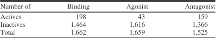
The resulting three data sets (binding, agonist, and antagonist;
Table 1) were provided to the modelers in three separate two-dimensional structure datafiles (2D SDF V2000) with QSAR-ready standardized structures in both Simplified Molecular Input Line Entry System (SMILES) and molecular format with atom coordi-nates (MOL) formats. The three-dimensional (3D) structures were also generated by energy minimization using MMFF94 forcefield and provided as 3D structure datafile (sdf) (V2000) files. In both the 2D and 3Dfiles, area under the curve (AUC) values were provided with the corresponding activity class (binary) and converted concen-tration values (AC50) indicating potency (Judson et al. 2015). In addition to the structures and data, each chemical was also given an associated CASRN, DTXSID identifier, preferred name, standar-dized InChI code, and a hashed InChI key of the Quantitative Structure-Activity Relationship (QSAR)-ready structures.
Each one of these data sets (available in Supplemental Material S2) could be used to build either continuous models predicting AUC values or categorical models predicting active and inactive classes. A list of chemicals in these three data sets could be consid-ered false negatives thus, could be removed by the participants dur-ing the modeldur-ing procedures. These potentially inconclusive chemicals (available in Supplemental Material S3) consisted of 21 chemicals from binding, 8 from agonist, and 14 from antagonist. Furtherfiltering based on clustering or other structure-based analy-sis was recommended to reduce the number of inactives and to decrease the bias between the two classes. The ToxCast™-derived data sets (provided in SDF file format), as well as the removed chemicals were made available for download at https://doi.org/ 10.23645/epacomptox.10321697.
Prediction Set, Structure Collection, and Curation of Lists of Interest
The initial CERAPP list was compiled from a library of over 50,000 chemicals that humans are potentially exposed to from lists of toxicological and environmental chemicals of interest. The main lists included the EPA’s Chemical and Product Categories data-base (U.S. EPA 2014a), thefirst version of the EPA’s Distributed Structure-Searchable Toxicity Database (DSSTox) (Richard et al. 2016;Richard and Williams 2002), and the Canadian domestic substance list (Environment Canada 2012). This library contained a total of 42,679 chemicals with known organic structures that, af-ter QSAR-ready standardization procedure and duplicates re-moval, was collapsed to 32,464 unique structures known as the CERAPP list (Mansouri et al. 2016a).
Table 1.Training set chemicals for binding, agonist and antagonist data sets.
Number of Binding Agonist Antagonist
Actives 198 43 159
Inactives 1,464 1,616 1,366
In CoMPARA, in addition to the lists included in CERAPP, we used the European inventory of existing commercial chemical sub-stances (EINECS) containing∼ 60,000 chemicals as a list of inter-est for in silico screening. We also incorporated ToxCast™ metabolites in the prediction set that had been generated as part of related ER studies (Leonard et al. 2018;Pinto et al. 2016). The goal of including metabolites in the CoMPARA project was to understand the effect of xenobiotic metabolism, which is lacking in mostin vitro assays. For ER screening efforts, this step was con-ducted post CERAPP in two different studies generating a total of 15,406 metabolite structures for ToxCast™ parent chemicals using ChemAxon Metabolizer (discontinued 2018) (ChemAxon, Ltd.) (Leonard et al. 2018;Pinto et al. 2016). After QSAR-ready stand-ardization and removal of duplicates, the CoMPARA list consisted of 55,450 QSAR-ready structures with unique CoMPARA integer IDs, including 6,592 nonredundant metabolite structures. This list matches 63,848 original (pre-QSAR-ready) chemical structures in the EPA’s DSSTox database, excluding the metabolites.
The CoMPARA chemical prediction set was provided in 2D and 3D SDF files. Data provided for each chemical included CoMPARA_IDs; structures in SMILES, MOL, and InChI code; and hashed InChI key formats for all chemicals. CASRNs, names, and DSSTox DTXSIDs were also provided when avail-able. This list of chemicals (identifiers and structures in SMILES format) is provided in Supplemental Material S4. The two QSAR-ready files as well as the original (prestandardization) structures file were made available for download athttps://doi. org/10.23645/epacomptox.10321697.
Evaluation Set, Literature Search, and Curation
To assess the developed models and their predictivity, an evalua-tion set with new chemicals (nonoverlapping with the training set) is required. Ideally, this new set would be the result of the same mathematical pathway model combining the 11 assays as that used for the training set. Because such a data set was not available, we decided to use data from the literature. Because the project was not a competition and the goal of this step was not to provide an in-depth comparison of the models, literature data could still be used to provide quality assessment and check for errors.
Large amounts of experimental data are available in the PubChem repository and related data sources. However, such public sources of chemical-biological data have varying levels of quality control, so additional curation and standardization are necessary (Williams and Ekins 2011). The EPA’s NCCT collected and curated PubChem data (64 sources), restructured it, and mapped the bioac-tivity values to related biological targets. In this effort, we started with ∼ 80,000 experimental values for AR activity, which mapped to about∼ 11,000 chemicals that we grouped by modality (agonist, antagonist) and hit call (active, inactive). To improve the consis-tency between the different PubChem entries and to add binding mo-dality, three rules were applied:
•In the case of multiple records for a test chemical, a mini-mum concordance of two out of three assay results was required to assign a positive activity score.
•An active agonist or antagonist was considered a binder.
•Inactive agonists and antagonists were considered nonbinders. The KNIME standardization workflow referenced earlier was applied to the chemical structures (Mansouri et al. 2016a;
McEachran et al. 2018). After removing ToxCast™ chemicals (used for the training set), the generated standard InChI codes matched 7,281 chemicals from the CoMPARA list (prediction set). This list of 7,281 chemicals, with associated data extracted from the literature, was used as the evaluation set. The removed ToxCast™ chemicals were mostly associated with ToxCast™ data only. The evaluation set chemicals were split into three
data sets based on the available experimental data. The resulting lists included 4,839 structures for agonist, 4,040 for antagonist, and 3,882 for binding. The numbers of active and inactive structures are summarized inTable 2.
AC50 values (lM) were available for 405 chemicals in the bind-ing data set, 167 chemicals in the agonist data set, and 340 chemicals in the antagonist data set. This process of preparing the evaluation set was conducted in KNIME. These three data sets (identifiers and structures in SMILES format) are provided in Supplemental Material S5. The SDFfiles have been made available for download athttps://doi.org/10.23645/epacomptox.10321925.
Participants and Modeling Methods
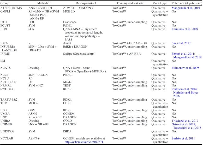
CoMPARA participants included a total of 70 scientists from 25 international research groups representing academia, governmen-tal institutions, and industry (See Supplemengovernmen-tal Material S1), including 15 groups that were involved in the related CERAPP pro-ject. The participating groups were located in 11 different coun-tries. The modelers were encouraged to use the provided training set and, preferably, apply free and open-source software tools that included detailed descriptions of the used methods and the employed applicability domain assessment. However, the applica-tion of proprietary commercial tools was also allowed. The different molecular descriptor calculation tools and the various modeling approaches employed are summarized inTables 3and4. Some of the groups collaborated with each other to submit common models. To produce more balanced data, most participants applied under-sampling approaches to reduce the number of inactive chemicals. For further details on the methods and approaches, see the full list of files submitted by the individual groups athttps://doi.org/10.23645/ epacomptox.10321982. Certain participants developed additional
Table 2.Evaluation set chemicals for binding, agonist, and antagonist data sets.
Number of Binding Agonist Antagonist
Actives 453 167 355
Inactives 3,429 4,672 3,685
Total 3,882 4,839 4,040
Table 3.Modeling approaches applied by the participating groups.
Abbreviation* Approach
Reference to specific method, if published
ANN Artificial neural networks —
ASNN Associative artificial neural networks
Tetko 2002;Tetko and Tanchuk 2002
DF Decision forest Hong et al. 2005,2004;Tong
et al. 2003;Xie et al. 2005
DT Decision trees —
GBM Gradient boosting method Berk 2008;Mazanetz et al. 2012
HC Hierarchical clustering Martin et al. 2008
kNN k nearest neighbors Cover and Hart 1967;
Kowalski and Bender 1972
LDA Linear discriminant analysis —
MLR Multilinear regression —
NB Naïve Bayes Murphy 2006
PLS Partial least squares Wold et al. 2001
PLSDA Partial least squares discriminative approach
Frank and Friedman 1993;
Nouwen et al. 1997
RBF Radial basis function Zakharov et al. 2014
RF Random forest Breiman 2001
SCR Self-consistent regression Lagunin et al. 2011
SVM Support-vector machines Cortes and Vapnik 1995
Note:—, No data.
models and published them or expressed their intent to publish them as separate manuscripts.
Evaluation Procedure
To ensure consistency and repeatability of the results, all molecular structures associated with the chemicals in the three data sets described above (training set, prediction set, and evaluation set) were processed using the same standardization workflow. This workflow was designed so that chemicals with the same standar-dized QSAR-ready structures would automatically have the same computational predictions (Fourches et al. 2010,2016;Mansouri et al. 2016a). Thus, chemicals from the different data sets could be matched using their respective QSAR-ready standard InChI codes.
After all predictions were made on the prediction set, the over-lapping chemicals with the evaluation set were used to evaluate the performance of the submitted models. The goal of this evaluation was not only to assess model accuracy but also to check for substan-tial procedural errors that could arise, such as mismatches among chemical identifiers, structures, and associated data. This step was intended to process the qualitative and the quantitative predictions separately. Only predictions within the applicability domain (AD), if provided, were considered, and there was no penalty for models with narrow AD. The main evaluation criteria were:
•Goodness-of-fit: statistics of the training set.
•Predictivity: statistics of on the evaluation set.
•Robustness: balance between goodness-of-fit and predictive ability.
Each of these three criteria was assigned a weight resulting in a score (S) ranging from 0 to 1
S = 0:3 × ðGoodness of fitÞ + 0:45
×ðPredictivityÞ + 0:25 × ðRobustnessÞ: (1) This score was not intended to rank the models but was designed by the organizers of the consortium mainly to evaluate the models’ predictivity and provide a rational basis to combine the predictions into a consensus in a later step. The weights were assigned to the different components in a way to give priority to the predictive ability on the evaluation set but not too high in comparison with the training set statistics because of the di ffer-ence between the two sets. The robustness or balance between the two was given the third rank but just slightly less weight than the goodness of fit because it highlights overfitting, which is almost as important a factor asfitting. However, a slightly differ-ent weight would most probably lead to the same results. To ensure equal contribution from the participants, the evaluation score accounted neither for the fraction of predicted chemicals nor the coverage of the AD, if provided.
Table 4.Tools and methods applied by the participating groups.
Group* Methods** Descriptors/tool Training and test sets Model type Reference (if published)
ATSDR_IRFMN ANN + SVM + DT ADMET + DRAGON 7 ToxCast™ Qualitative Manganelli et al. 2019
CMPLI RF + kNN + NB + SVM
MLR + PLS + ANN + RF
MOE 3D ToxCast™ Qualitative +
quantitative NA
DTU PLR Leadscope ToxCast™, under sampling Qualitative NA
ECUST SVM PaDEL ToxCast™ Qualitative NA
IBMC SCR QNA + MNA + PhysChem
properties (topological length, volume and lipophilicity) + PASS
Qualitative Filiminov et al. 2009
IDEA RF Ambit ToxCast™ + ExC APE-DB Qualitative Sun et al. 2017
INSUBRIA_ LANZHOU
kNN + LDA + SVM + RF + DT
RdKit + DRAGON ToxCast™, under sampling Qualitative NA
IRFMN SARpy (Structural alerts) ToxCast™ + AR RBA Qualitative Ferrari et al. 2011;
Manganelli et al. 2019
LM Qualitative +
quantitative NA
NCATS Docking + QNA + Keras Theano +
DOCK + Open Eye + MOE Dock
ToxCast™ Qualitative Filimonov et al. 2009
NCCT kNN + PLSDA PaDEL ToxCast™ Qualitative NA
NCSU RF ToxCast™ Qualitative NA
NCTR_DUT DF Mold2 ToxCast™, under sampling Qualitative NA
NRMRL SVM + HC TEST ToxCast™, under sampling Qualitative NA
SWETOX RF RDKit ToxCast™ Qualitative Carlsson et al. 2014;
Norinder and Boyer 2016
TARTU-1&2 SVM RDKit ToxCast™, under sampling Qualitative NA
TUM MLR + CDK ToxCast™ Qualitative +
quantitative NA
UFG GBM RDKit ToxCast™, under sampling Qualitative NA
UMEA ASNN OCHEM ToxCast™ Qualitative NA
UNC RF + RBF DRAGON ToxCast™, under sampling Qualitative NA
UNIBA Docking GOLD ToxCast™, under sampling Qualitative Trisciuzzi et al. 2017
UNIMIB kNN + NB + RF DRAGON ToxCast™, under sampling Qualitative Grisoni et al. 2019,
Todeschini et al. 2015
UNISTRA SVM ISIDA ToxCast™ Qualitative +
quantitative NA
VCCLAB ASNN + OCHEM, models are available at
http://ochem.eu/article/102271
ToxCast™ Qualitative +
quantitative
Sushko et al. 2011
*Groups are listed alphabetically by group acronym. See Supplemental Material 1 for full group names. **Methods names as provided inTable 3.
For the qualitative models, this general formula was translated into commonly used classification parameters as discussed below. However, for the quantitative models, the predictions based on the training set data (ToxCast™ AUC values) were different from those of the evaluation set data (AC50 values). To ensure consistency and validity of the evaluation procedure, the qualita-tive and quantitaqualita-tive models and predictions were processed sep-arately as explained below.
Qualitative Evaluation Procedure
The categorical predictions were evaluated using statistical indi-ces commonly proposed in the literature (Ballabio et al. 2018). These indices are calculated from the confusion matrix, which collects the number of samples of the observed and predicted classes in the rows and columns, respectively. The classification parameters are defined using the number of true positives (TP), true negatives (TN), false positives (FP), and false negatives (FN). The resulting parameters were the balanced accuracy (BA), specificity (Sp), and sensitivity (Sn) calculated as follows:
The BA is given by:
BA =ðSn + SpÞ
2 , (2)
where the sensitivity (Sn), or true positive rate (TPR) is given by:
Sn =TP + FNTP , (3)
and the specificity (Sp), or true negative rate (TNR) is given by:
Sp =TN + FPTN : (4)
For classification models, not only is the average of the Sn and Sp explained by the BA important, but also the balance between them. Therefore, to fully assess the predictivity of the models, the three criteria are included in the general scoring func-tion S, calculated as follows:
Goodness of fit = 0:7 × ðBATrÞ + 0:3 × ð1 − jSnTr− SpTrjÞ,
ð5Þ Predictivity = 0:7 × ðBAEvalÞ + 0:3 × ð1 − jSnEval− SpEvaljÞ,
ð6Þ Robustness = 1− jBATr− BAEvalj, ð7Þ
whereTr stands for training set and Eval stands for evaluation set, attributing weight not only to the BA but also to the balance between Sn and Sp to account for the reliability of the model in predicting actives as well as inactives.
Quantitative Evaluation Procedure
Active chemicals with available quantitative information (AC50 values) from the mined literature sources (405 chemicals in the binding data set, 167 chemicals in the agonist data set and 340 chemicals for the antagonist data set) were considered for this step to evaluate the quantitative models’ predictivity. The analysis of the quantitative results conducted during the CERAPP project showed some differences between the AC50 values collected from the literature and the AC50 values converted from the predicted AUC scores. These differences include the fact that the AUC scores represented the results of multiple assays that were com-bined to overcome assay interference and cytotoxicity, whereas the
literature data is a one source per assay most of the time. In addi-tion, the ToxCast™ assays’ limiting dose of 100 lM makes these assays insensitive to“very weak” actives that are reported in the lit-erature to have AC50 values beyond that threshold. Thus, to con-duct a quantitative evaluation of the predictions using the literature data without underestimating the accuracy of the predictions, the two types of results needed to be converted to a more consistent data type. The multiclass approach presented in this work convert-ing both the literature data and the predicted AUC values tofive categories with approximately similar potencies was built on the CERAPP approach (Mansouri et al. 2016a). This approach is com-monly used in the QSARfield to predict end points that are hard to model on a continuous scale and to avoid underestimating predic-tivity (Benigni 2003; Dunn 1990; Kowalski 2013;Waterbeemd 2008). This approach was applied in CoMPARA to avoid the same problem when evaluating the models that were trained on the ToxCast™-based AR pathway model (AUC values) using litera-ture data. Both literalitera-ture (evaluation set chemicals with quantita-tive information) and predicted data sets were categorized intofive potency activity classes: inactive, very weak, weak, moderate, and strong [example reference chemicals with different potency levels are available in Judson et al. and Kleinstreuer et al. (Judson et al. 2015;Kleinstreuer et al. 2017)]. Thesefive classes were used to evaluate the quantitative predictions.
The thresholds determined in the CERAPP project were applied to the concentration-response values (AC50) from the literature:
•Strong: Activity concentration below 0:09 lM
•Moderate: Activity concentration between 0.09 and 0:18 lM
•Weak: Activity concentration between 0.18 and 20lM
•Very Weak: Activity concentration between 20 and 800lM
•Inactive: Activity concentration higher than 800lM For the training set, the AUC values were converted intofive potency classes based on the following thresholds:
•Strong: AUC equal to or above 0.75
•Moderate: AUC between 0.75 and 0.65
•Weak: AUC between 0.65 and 0.25
•Very weak: AUC between 0.25 and 0.09
•Inactive: AUC below 0.09
Although the ToxCast™ single assays were limited to a maxi-mum concentration of 100lM, similar to CERAPP, active chemi-cals with an AUC score below 0.25 are considered “very weak.” However, for the lack of chemicals in the 0.25 to 0.5 AUC range (weak in CERAPP), this arbitrary range for weak actives was extended to 0.65. The five classes were assigned labels from 1 (inactive) to 5 (strong), and then the models were evaluated as mul-ticlass categorical models in binding, agonist, and antagonist modes separately. The above-mentioned formulas for calculating Sn, Sp, and BA were applied to each of the classes, and then the average values (for thefive classes) were inserted into the scoring function. Consensus Modeling
After being evaluated separately according to the defined strat-egy, each model was given a score (S) for predictions within its AD. This score was used in the consensus modeling step as a weighting factor. Using these weights, the predictions within the AD of the submitted models were combined into a single consen-sus model separately for each modality (binders, agonists, and antagonists). For each chemical in the prediction set, the consen-sus category was decided by the weighted majority rule: the chemical was assigned the class with the highest average score of the models predicting it (class with the highest average score was selected). This average score excluded the models that did not provide a prediction for the chemical in question.
The consensus model predictions were evaluated using the same evaluation set and procedure used to evaluate the individual
models, and their performances were compared to the single models. Analyses of the accuracy trends and concordance (frac-tion of consistent predic(frac-tions) among the predic(frac-tions of the di ffer-ent models were also conducted. Considering only the models that provided predictions, the sum of the concordance among models for actives and inactives should be equal to 1.
Generalization of the Consensus and Implementation in OPERA
To use the consensus models beyond the initial prediction set, the combined predictions were used to train generalized models capable of replicating the original consensus. This procedure was achieved by applying a weighted k-nearest-neighbor (kNN) approach tofit the classification models based on the majority vote of the nearest neighbors. This approach has the advantage of resembling read-across, which is a broadly accepted data-gapfilling tool in regula-tory agencies (Ball et al. 2016;Patlewicz et al. 2017). In addition, kNN models can also satisfy thefive OECD principles for QSAR modeling due to their nonambiguous algorithm, high accuracy, and interpretability (Buttrey 1998;Cover and Hart 1967). Furthermore, being distance-based (dissimilarity), the weighted kNN approach fits the purposes of extending the consensus predictions to new chemicals and providing the exact same prediction for the chemicals that already have a consensus model prediction. This goal is achieved by considering thefirst nearest-neighbor prediction if the distance is zero (100% similarity). An applicability domain index is also provided to assess the similarity of the predicted chemical to the nearest neighbors.
PaDEL (version 2.21) and CDK (version 2.0) were used to cal-culate two-dimensional molecular descriptors (Guha 2005; Yap 2011). Because PaDEL uses a previous version of CDK (1.5), overlapping descriptors between it and CDK2 were excluded. The union of the PaDEL descriptors (1,444) and CDK2 (287) resulted in a total of 1,616 variables that were laterfiltered for low variance and missing values.
Here, kNN was coupled with genetic algorithms (GA) to select a minimized optimal subset of molecular descriptors. GA begins with an initial random population of chromosomes, which are bi-nary vectors representing the presence or absence of molecular descriptors. An evolutionary process is then simulated to optimize a defined fitness function and new chromosomes are obtained by coupling the chromosomes of the initial population with genetic operations such as crossover and mutation (Ballabio et al. 2011;
Leardi and Lupiáñez González 1998).
The best models were selected and implemented in OPERA, a free and open-source suite of QSAR models (Mansouri et al. 2016b,2018). Both OPERA’s global and local AD approaches, as well as the accuracy estimation procedure, were applied to the predictions (Mansouri et al. 2018). The global AD is a Boolean index based on the leverage approach for the whole training set, whereas the local AD is a continuous index in the [0–1] range based on the most similar chemical structures from the training set (Mansouri et al. 2018).
Results and Discussion
Received ModelsThere was a total of 91 models submitted by the participating groups. Each submission consisted of predictions for the full or fraction of the prediction set using one or multiple models, as well as the related documentation with various levels of detail. All sub-mitted results for the prediction set are provided in Supplemental Material S6. The full list offiles submitted by the participants is available athttps://doi.org/10.23645/epacomptox.10321982. The
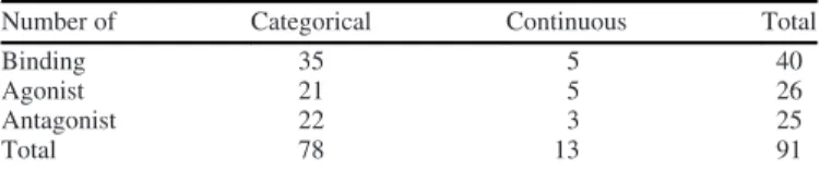
submissions included categorical and continuous predictions from binding, agonist, and antagonist models as shown inTable 5.
The number of categorical models submitted greatly exceeded the number of continuous models. This difference is due to the dif-ficulty of modeling the low number of AUC values greater than zero in the provided training set (ToxCast™ data). All participating groups provided at least one binding model. Thus, the number of binding models is higher than the number of either agonist or an-tagonist models. This higher number is also due to the biased train-ing data, which included low numbers of active agonists and antagonists. As described above, the number of active binders is the union of both active agonists and antagonists.
Results of the Evaluation Procedure
The evaluation procedure described above was applied to the cat-egorical and continuous predictions provided by the participants. The goal of this step was to assess the accuracy of the predictions that, in a later step, were combined into the consensus models. Thus, the evaluation procedure was not designed to reflect the uneven coverage of the prediction set, and application of an AD was encouraged.
The first application of this evaluation procedure revealed models that suffered from mishandling of data that might occur during the modeling process. Such errors led to a severe decrease in prediction accuracy and included mismatches between the IDs of the prediction set chemicals and their associated predictions, as well as misinterpretation (inverting or mismatching) of the dif-ferentfields contained in the provided files (training and predic-tion sets) introduced by certain automated procedures. Because the goal of the project was not to compete, but rather to collabo-rate, the submitters of the models with such issues were notified to correct them to allow for a better contribution toward the con-sensus. Thefinal, corrected submissions were used to produce the statistics provided in Supplemental Material S7. The results of the evaluation procedure, discussed below, are also available at
https://doi.org/10.23645/epacomptox.10321994. Qualitative Models
As mentioned earlier, all participating groups built categorical binding models. Furthermore, certain groups, such as IRFMN and ATSDR, collaborated with others to provide additional mod-els (Manganelli et al. 2019). For binding activity, ∼ 85% of the models achieved a BA above 0.8 for the training set, and about 70% of them achieved a BA above 0.7 for the evaluation set. On average, the BA of most models decreased ∼ 15% for the evalua-tion set relative to the training set. We consider this decrease to be negligible based on the differences between the training set data (which are based on the AUC values of the ToxCast™ AR pathway model that combines multiple assays) and the evaluation set data (which are consensus hit calls from the literature or rely on only one record for a particular chemical with unknown repro-ducibility). With this high predictivity and balance between train-ing and evaluation set performance increastrain-ing their robustness,
∼ 75% of the binding models reached a score of 0.75.
The agonist models showed a higher performance in compari-son with the binding models. Indeed, all agonist models had a training BA above 0.8, and 95% of them achieved a BA above
Table 5.Summary of the submitted models.
Number of Categorical Continuous Total
Binding 35 5 40
Agonist 21 5 26
Antagonist 22 3 25
0.75 on the evaluation set. This performance brings the average difference between training and test BA down to 0.1, indicating lower risk of overfitting. Most ( ∼ 95%) of the agonist models achieved a score above 0.85 (Figure 2).
Although the data sets contained more active antagonists in comparison with agonists, the general performance of the antago-nist models was inferior. This inferiority was reflected in the evaluation set performance, because only two models reached a BA of 0.75, which affected their robustness (0.24 average differ-ence between the training and evaluation BAs). However, the av-erage and median scores reached 0.78 and 0.79 respectively, which shows high general performance of the models (Figure 2).
Most of the submitted categorical models (agonist, antagonist, and binding) provided predictions for the majority of the predic-tion set chemicals (>90%). Some of the participants who submit-ted more than one model, such as NCATS and UNIMIB, opsubmit-ted for a low coverage with high accuracy and a high coverage with lower accuracy. Additional details about the performance of the models is provided in Supplemental Material S7.
Quantitative Models
The quantitative models were converted into multiclass categori-cal models as described in the Methods section. The overall per-formance of the thirteen models across the three modalities (agonist, antagonist, and binding) was lower than that of the bi-nary categorical models. The binding models performed a bit bet-ter than the agonist and antagonist models. Indeed, four binding models out offive obtained a score above 0.6, whereas only one agonist and one antagonist model performed that well (Figure 3). The predictive accuracy of these models was also assessed on the five classes separately (details available in Supplemental Material S7). This analysis showed that most models exhibited BAs of approximately 0.5 for thefive classes, with the binding models exhibiting slightly better performance (0.7–0.78) in identifying inactives.
Consensus Modeling
Based on their low number and average performance in compari-son with the categorical models, the recommendation would be that the continuous models should be used individually. A
continuous consensus model can be derived only from a more concordant set of models. Thus, for the sake of accuracy and sistency of the predictions, only the categorical models were con-sidered for the consensus step. Before combining the categorical predictions into a consensus, we checked the coverage and con-cordance among the models. As shown inFigure 4, all chemicals in the prediction set are covered by at least 11 models. Moreover, most chemical structures can be predicted by 18–20 agonist and antagonist models. For binding, most chemicals were predicted by 28–31 models. This high coverage provides a good basis for the consensus model and strengthens the statistical relevance of the combined predictions.
The concordance among the models is also an important crite-rion for combining the predictions. In fact, chemicals predicted with high concordance among numerous models built using dif-ferent modeling approaches can inform on accuracy (Mansouri et al. 2016a).Figure 5shows that most binding, agonist, and an-tagonist categorical predictions are at least 90% concordant. Because most models were associated with comparable scores, the average score used to categorize chemicals was largely in
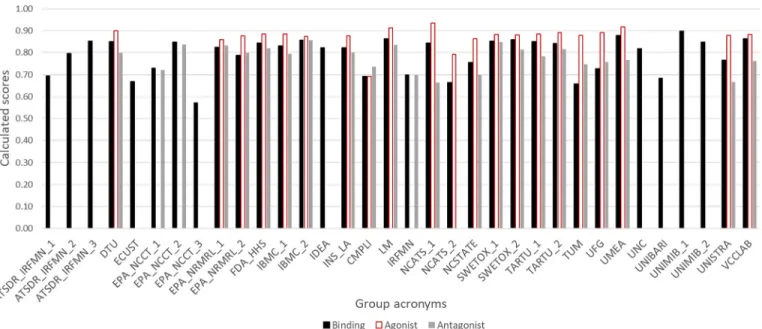
Figure 2.Scores of the categorical binding (black), agonist (white) and antagonist (gray) models based on the evaluation set and the scoringEquation 1.
Figure 3.Scores of the continuous binding (black), agonist (white) and antagonist models based on the evaluation set and the scoringEquation 1
agreement with model concordance; i.e., the average score for actives was high when the concordance among the models with active predictions was high, and vice versa. A few exceptions were noted when model concordance was around 0.5, which indi-cated that only one or two models were driving the classification. Thus, based on these statistical observations about the concord-ance between the models, it can be concluded that it is possible to combine the categorical predictions into consensus agonist, an-tagonist and binding predictions.
Consensus Predictions
The predictions from the binding, agonist, and antagonist cate-gorical models were atfirst combined independently based on the calculated scores. Because the participants provided uneven frac-tions of the prediction set, the resulting predicfrac-tions for each of the 55,450 chemical structures were based on different contribut-ing models. Thus, predictions from the same model can be asso-ciated with different weights across the prediction set. After generating the consensus predictions for the whole prediction set,
the same evaluation procedure described previously was applied to each of the single models. The resulting statistical details are reported in Supplemental Material S7 as CONSENSUS_1. All obtained parameters, including the BA for the training and evalu-ation sets as well as the corresponding score, were around the top values obtained for the single models.
In a second step, to improve consistency among the agonist, antagonist, and binding predictions across the whole set of 55,450 chemicals, the following set of rules were applied:
•If a chemicali was predicted to be an active agonist or antag-onist with a concordance below 70%, but an inactive binder with a concordance above 70%, it was considered an inactive agonist or antagonist, respectively.
•If a chemicali was predicted to be an active agonist or antago-nist with a concordance above 70%, but an inactive binder with a concordance below 70%, it was considered an active binder. After applying these corrections to the consensus predictions, the total numbers of actives and inactives changed slightly for the three modalities (Table 6). However, the overall statistics as reported as CONSENSUS_2 in Supplemental Material S7 remained almost unchanged. This result is because most of the corrected predictions are not included in the evaluation set. The evaluation results of thefinal consensus predictions are reported in Table 7. The final consensus for the whole prediction set (identifiers and structures in SMILES format) are provided in Supplemental Material S8, and the SDF files are available at
https://doi.org/10.23645/epacomptox.10322012.
Because the training and evaluation sets were designed such that active agonists and antagonists were considered active bind-ers, the corrected predictions can be considered more consistent with these two data sets. However, chemicals with inactive bind-ing prediction and active agonist or antagonist that are all below 70% concordance were not changed. Also, certain chemicals were predicted to be active binders but inactive in both agonist and antagonist modalities. This circumstance was also noticed in the CERAPP predictions and was resolved by classifying these substances as low potency binders (Mansouri et al. 2016a). Similarly, certain chemicals were predicted to be active agonists and antagonists simultaneously. Such chemicals were also pres-ent in the ER and AR ToxCast™ data, as well as CERAPP predic-tions, and were considered to be strong in one modality but weak in the other.
Table 7shows a noticeable drop in Sn and in the associated BA result for the whole evaluation set with its five potency classes. However, this drop does not indicate low performance of the single models or the resulting consensus predictions. It is more of an indi-cation of differences between the two data sets. Usually, assay technology and other experimental differences can cause such dis-cordance for certain chemicals. However, in this case, the low sen-sitivity of the consensus model on the evaluation set that led to the drop in accuracy in comparison with the training set is most prob-ably due to the differences in the ranges of testing between ToxCast™ and the literature sources. Another cause of the differ-ence between the two data sets is that the ToxCast™ data is a result of multiple assays that were combined based on a pathway model designed to avoid assay interference and cytotoxicity leading to false positives. This result can occur when chemicals are tested at
Figure 4.Histogram showing the distribution of the number of binding (black), agonist (white) and antagonist (gray) models covering the prediction set (minimum of 11 models for agonist and antagonist and 20 for binding).
Figure 5.Histogram showing the distribution of the concordance of the binding (black), agonist (white) and antagonist (gray) single models.
Table 6.Total numbers of predicted actives and inactives before and after corrections.
Correction
Binding Agonist Antagonist
Actives Inactives Actives Inactives Actives Inactives
Before 9,878 45,572 2,239 53,211 12,705 42,745
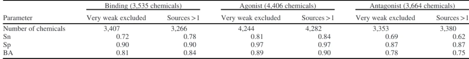
high concentrations, leading to cell stress known as a“burst of ac-tivity” from turning multiple assays on at the same time (Judson et al. 2016). Thus, it is highly probable that at least some of the very weak actives in the evaluation set reported in the literature with high AC50 are, in reality, false positives that should be dis-counted. Additionally, as noticed in CERAPP, the increase in the number of sources in the literature data can provide information about the repeatability of the results and thus about the accuracy. These two hypotheses were evaluated by assessing the accuracy of the models (BA, Sn, and Sp) for the evaluation set after removing the chemicals in the“very weak” potency class and the chemicals with only one source, separately. The results of this analysis are summarized inTable 8.
Table 8shows that for all three modalities and in both cases (removal of very weak and single sources), the Sn of the models increased, which in turn increased the BA. Except for the agonist mode with the removal of single sources, which is a single case out of six, the Sn showed an increase of 7%–12%. This increase can be considered as a statistically significant increase in Sn after the removal of 2%–7% of the data set. Thus, it can be concluded that a significant percentage of a) the “very-weak” chemicals reported in the literature are false positives according to the de fi-nition applied in this project and b) the literature data with a reported single source is less reliable. Similar to CERAPP find-ings,Figure 6shows that only a small fraction of the CoMPARA list is predicted to be active binders with >75% concordance between the models. Also, most of the inactive predictions, which are the majority of the list, are associated with high concordance. Thus, the models are more in agreement for the inactive predic-tions. Thisfinding can be explained by the imbalanced training data and the uneven sensitivity of the models to weak actives. Additionally, because most of the models were built using ToxCast™ data, their sensitivity will be limited by its tested con-centration ranges (≤100 lM).
Coverage and Contribution of Single Models to the Consensus
The evaluation set that was initially used to evaluate the single models covered only a small fraction of the full prediction set. Therefore, to gain insight into the contribution of the single mod-els, the predictions provided by each of them were evaluated against the consensus for the full CoMPARA list. Sn, Sp, BA, and scores were calculated using the same previously mentioned functions.Figure 7shows the score and coverage of each one of the binding models in comparison with the full list of the consen-sus predictions. The full results of this procedure, including simi-larfigures for agonist and antagonist modalities, are reported in Supplemental Material S9. Thesefigures show the consistency of
the different models across the full list of 55,450 chemicals in the prediction set. This information is also an indication of the con-cordance of the single models among each other. The analysis of these figures in comparison withFigure 2, representing the per-formance of the models on the training and evaluation sets, shows similar trends for most models. Thisfinding means that the mod-els are behaving in a consistent way across the full prediction set in comparison with the training and evaluation sets. However, certain models showed a higher concordance with the consensus predictions, whereas others were more consistent with the train-ing and evaluation set. The trends of such models confirm that the scores obtained at the initial evaluation procedure for each individual model did not drive the consensus predictions, but the general concordance (majority rule) did.
Accuracy and Limitations: Analysis of High and Low Concordance Chemicals
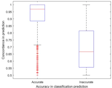
The analysis of the low concordance chemicals did not reveal any particular structural similarity. This finding is understandable because the ToxCast™ chemicals, used as a training set, were pur-posely selected to cover a wide range of chemical classes and uses (Richard et al. 2016). Thus, it is highly improbable that a large number of models based on different machine learning approaches and molecular descriptors would have similar coverage and accu-racy trends relative to specific chemical features. However, the analysis of concordance in terms of the accuracy of prediction in the evaluation set revealed that the models were more discordant for inaccurate predictions.Figure 8shows that the concordance is generally above 90% for accurately predicted chemicals. There are certainly a number of exceptions that contradict this observation and that cannot be linked only to situations where the majority of models are generating wrong predictions but also to known di ffer-ences between the training and evaluation sources. For example, hydroxyflutamide (CAS52806-53-8 and DTXSID8033562), a known antiandrogen drug, and confirmed as a strong antagonist with an AUC (ToxCast™ combined assays) score of 0.999 and a literature AC50 of 0:262 lM (U.S. EPA 2019e,2019f;Wikipedia 2018). Hydroxyflutamide is, as expected, predicted by CoMPARA consensus to be an AR antagonist with a 0.95 concordance (20/21 antagonist models). However, in the collected literature data, hydroxyflutamide is also a very weak agonist with reported AC50 of 23:85 lM. However, in the CoMPARA consensus agonist pre-dictions, it is considered as inactive with a concordance of 0.95 (20/21 agonist models), which is consistent with to ToxCast™ AUC score of 0.001 (U.S. EPA 2019f). This example shows that the sensi-tivity of the CoMPARA consensus models is more similar to the AUC score assessment, which is based ToxCast™ combined assays, rather than that in reported literature, which is usually based on a
Table 7.Statistics of the corrected consensus predictions using the whole available evaluation set.
Parameter
Binding Agonist Antagonist
Training set Evaluation set Training set Evaluation set Training set Evaluation set
Sn 0.98 0.65 0.95 0.74 1.00 0.61
Sp 0.96 0.90 0.99 0.97 0.96 0.87
BA 0.97 0.78 0.97 0.86 0.98 0.74
Table 8.Statistics of the consensus predictions after removing the“very weak” actives from the evaluation set.
Parameter
Binding (3,535 chemicals) Agonist (4,406 chemicals) Antagonist (3,664 chemicals)
Very weak excluded Sources >1 Very weak excluded Sources >1 Very weak excluded Sources >1
Number of chemicals 3,407 3,266 4,244 4,282 3,353 3,380
Sn 0.72 0.78 0.81 0.84 0.69 0.62
Sp 0.90 0.90 0.97 0.97 0.87 0.87
single assay and corresponding independent reference. Another sim-ilar example is bicalutamide (CAS90357-06-5 | DTXSID2022678) (U.S. EPA 2019c,2019d;Wikipedia 2019b). However, this compar-ison does not mean that all very weak actives are mispredicted. Aldosterone, for example, and many others are reported in the litera-ture as very weak antagonists with AC50 values above 60lM and predicted by CoMPARA’s antagonist consensus as actives with con-cordances above 0.75 (U.S. EPA 2019a,2019b;Wikipedia 2019a).
As previously noted, the concordance around the inactive pre-dictions is generally high for most cases. Hence, to reveal any trends in the active predictions, a box plot for the concordance against the potency of binders was plotted for the evaluation set chemicals (Figure 9). This analysis showed that the concordance for moderate and strong binders is clearly higher than for very weak and weak ones. Similar trends were noticed for the agonist and antagonist predictions. The decreased accuracy for the low
potency chemicals can explain the low sensitivity of the consen-sus predictions as discussed above, and the low concordance can be an indication of low accuracy. However, asFigure 8 shows, there are accurate predictions associated with low concordance and inaccurate predictions associated with high concordance. This finding is comparable to the AD assessment, which helps provide the user with context based on the assumption that pre-dictions in the AD are generally more accurate than those outside the AD. The AD is not a definitive judgment on the accuracy because certain predictions in the AD might be inaccurate, and vice versa (Sahigara et al. 2014). Similarly,Figure 9shows that moderate and strong predictions are generally associated with higher concordance than are weak and very weak predictions.
Figure 6.Histogram showing the distribution of the concordance between the binding models over the active predictions.
Figure 7.Histogram showing the coverage and S-score of the single binding models in comparison with the consensus binding predictions for the full CoMPARA set.
Figure 8.Box plot showing the correlation between concordance and accuracy of prediction for the evaluation set chemicals. The box represents the interquar-tile range. The lower and upper box boundaries represent the 25th and 75th per-centiles, respectively. The horizontal line splitting the box represents the median value. The upper and lower whiskers represent the minimum and maxi-mum values, respectively. Outliers are represented by the + symbol.