HAL Id: hal-00296008
https://hal.archives-ouvertes.fr/hal-00296008
Submitted on 22 Aug 2006
HAL is a multi-disciplinary open access
archive for the deposit and dissemination of
sci-entific research documents, whether they are
pub-lished or not. The documents may come from
teaching and research institutions in France or
abroad, or from public or private research centers.
L’archive ouverte pluridisciplinaire HAL, est
destinée au dépôt et à la diffusion de documents
scientifiques de niveau recherche, publiés ou non,
émanant des établissements d’enseignement et de
recherche français ou étrangers, des laboratoires
publics ou privés.
fluorescence (TD-LIF) to measurement of HNO3, ?alkyl
nitrates, ?peroxy nitrates, and NO2 fluxes using eddy
covariance
D. K. Farmer, P. J. Wooldridge, R. C. Cohen
To cite this version:
D. K. Farmer, P. J. Wooldridge, R. C. Cohen. Application of thermal-dissociation laser induced
fluorescence (TD-LIF) to measurement of HNO3, ?alkyl nitrates, ?peroxy nitrates, and NO2 fluxes
using eddy covariance. Atmospheric Chemistry and Physics, European Geosciences Union, 2006, 6
(11), pp.3471-3486. �hal-00296008�
www.atmos-chem-phys.net/6/3471/2006/ © Author(s) 2006. This work is licensed under a Creative Commons License.
Chemistry
and Physics
Application of thermal-dissociation laser induced fluorescence
(TD-LIF) to measurement of HNO
3
, 6alkyl nitrates, 6peroxy
nitrates, and NO
2
fluxes using eddy covariance
D. K. Farmer1, P. J. Wooldridge1, and R. C. Cohen1,2
1Department of Chemistry; University of California, Berkeley, Berkeley, CA, 94720, USA
2Department of Earth and Planetary Science; University of California, Berkeley, Berkeley, CA, 94720, USA
Received: 22 December 2005 – Published in Atmos. Chem. Phys. Discuss.: 12 April 2006 Revised: 23 June 2006 – Accepted: 28 July 2006 – Published: 22 August 2006
Abstract. Nitrogen exchange between the atmosphere and biosphere directly influences atmospheric composition. While much is known about mechanisms of NO and N2O
emissions, instrumentation for the study of mechanisms con-tributing to exchange of other major nitrogen species is quite limited. Here we describe the application of a new technique, thermal dissociation-laser induced fluorescence (TD-LIF), to eddy covariance measurements of the fluxes of NO2, total
peroxy acyl and peroxy nitrates, total alkyl and multifunc-tional alkyl nitrates, and nitric acid. The technique offers the potential for investigating mechanisms of exchange of these species at the canopy scale over timescales from days to years. Examples of flux measurements at a ponderosa pine plantation in the mid-elevation Sierra Nevada Mountains in California are reported and used to evaluate instrument per-formance.
1 Introduction
The exchange of nitrogen between the biosphere and at-mosphere affects both oxidative atmospheric chemistry and ecosystem nutrient dynamics, with potential indirect effects on the carbon cycle and climate (Ollinger et al., 2002; Vi-tousek et al., 1997). Nitrogen enters ecosystems through ap-plication of fertilizer, biotic nitrogen fixation of N2, or
atmo-spheric deposition of gaseous or particulate ammonium and oxidized nitrogen, is rapidly cycled in both organic and in-organic forms, and is known to be released from ecosystems to the atmosphere through direct plant emissions of NO or NO2, and as a by-product of soil microbial transformations,
namely as NO or N2O via nitrification and denitrification.
As N is commonly the limiting nutrient for plant growth in forest ecosystems, increased N deposition also increases car-Correspondence to: R. C. Cohen
(rccohen@berkeley.edu)
bon uptake. (Vitousek et al., 1997). This effect has clear implications as the CO2level in the atmosphere continues to
rise concurrently with increased anthropogenic N emission and consequent increased N deposition to ecosystems (Siev-ering et al., 2001). However, because N emissions contribute to ozone formation, increased N deposition associated with those emissions may also be accompanied by increased de-position of ozone. The negative impact of ozone on plant health may offset the positive effects of N deposition on C uptake (Ollinger et al., 2002). As N deposition may lead to increased N2O emissions and soil respiration, the net C
up-take may be further offset (Fenn et al., 1998; Schlesinger and Andrews, 2000). The continued increase in anthropogenic emissions of reactive nitrogen into the atmosphere and nitro-gen deposition has lead to concerns regarding nitronitro-gen satu-ration, which may decrease plant health, increase greenhouse gas emissions, and affect water quality (Aber et al., 1998).
Bulk wet and dry nitrate/ammonium deposition has been quantified over numerous ecosystems (e.g. Bobbink et al., 1992; Bytnerowicz and Fenn, 1996; Holland et al., 2005; Shepard et al., 1989 and references therein). More detailed experiments have focused on NO and N2O because of their
clear soil sources, the greenhouse warming potential of N2O,
and the availability of commercial detectors (e.g. Davidson and Kingerlee, 1997; Hanson and Lindberg, 1991; Ludwig et al., 2001; Mosier et al., 2004 and references therein). How-ever, ammonia (NH3)and the reactive nitrogen oxides (NOy
= NO + NO2+ PAN + other peroxy nitrates + alkyl nitrates
+ nitric acid + N2O5+ . . . ) are significant contributors to N
dry deposition, and recent research indicates that surface in-teractions affect atmospheric concentrations and partitioning of these species. For example, extreme changes in the at-mospheric reactive nitrogen budget following biomass burn-ing or rain events have been observed (Bertram et al., 2005; Jaegle et al., 2004; Zhang et al., 2002). Few studies have investigated the magnitude and mechanisms of ecosystem-scale exchange of NO2, peroxy nitrates, alkyl nitrates or
HNO3, likely because of the absence of techniques for
mea-surement of these reactive nitrogen oxide species with both adequate sensitivity and minimal day-to-day maintenance requirements to enable application to ecosystem-scale flux measurements. Eddy covariance (EC) is the most direct method of measuring the exchange of compounds between the atmosphere and earth’s surface. (Dabberdt et al., 1993). This technique has stringent requirements for measurements of vertical wind speed and concentration, requiring obser-vations that are fast (>1 Hz), sensitive, portable, and free of interferences (Baldocchi et al., 1988; McMillen, 1988). EC flux measurements of NOy, NO, and NO2 fluxes have
been reported (e.g. Delany et al., 1986, Horii et al., 2004; Munger et al., 1996; Rummel et al., 2002). Most other stud-ies of N fluxes have used enclosure or indirect estimation techniques, including gradient measurements or resistance modeling (Hanson and Lindberg, 1991; Wesely and Hicks, 2000).
The most extensive measurements are those described by Munger et al. (1996), who observed NOy using
eddy covariance at both remote (0.003 ppb m s−1
summer-time net dry NOy flux, Schefferville, Quebec1) and rural
(0.023 ppb m s−1summertime, 0.022 ppb m s−1 wintertime,
Harvard Forest) environments. Model results by Munger et al. (1998) indicate that deposition of hydroxyalkyl nitrates, HNO3 from heterogeneous reactions of N2O5 and HNO3
from oxidation of NO2by OH contributed comparably to
to-tal NOydeposition during summer at Harvard Forest. Horrii
(2002) found that while the NOyflux at Harvard Forest was
explained by HNO3 deposition with minor NO2 and PAN
contributions for unpolluted background flows, up to 50% of the NOy flux in polluted flows was not accounted for by
NO2, PAN, and HNO3, and was therefore likely due to alkyl
or hydroxyalkyl nitrates and other peroxy or peroxy acyl ni-trates.
All published HNO3flux measurements have been either
inferential (e.g. Lefer et al., 1999; Tarnay et al., 2001) or in-direct (e.g. Huebert et al., 1988; Janson and Granat, 1999; Nemitz et al., 2004; Pryor et al., 2002). Tarnay et al. (2001) used inferential flux measurements at Lake Tahoe, CA, and determined that dry deposition of HNO3is the major source
of atmospheric N to the lake. HNO3deposition velocities of
7.6 cm s−1were measured at Niwot Ridge using the flux
gra-dient approach (Sievering et al., 2001). Pryor et al. (2002) used both gradient and relaxed eddy accumulation (REA) techniques to measure HNO3fluxes. While downward fluxes
were generally observed, Pryor et al. also observed HNO3
ef-flux, potentially due to a chemical flux divergence involving HNO3-NH3-NH4NO3reactions and gas-particle nitrate
par-titioning, as has also been suggested in several other studies of upward HNO3 fluxes (Brost et al., 1988; Huebert et al.,
1Note that 1 ppb m s−1= 147 µmol m−2hr−1= 0.57 µg (N)m−2
s−1.
1988; Neftel et al., 1996; Nemitz et al., 2004; Van Oss et al., 1998).
The sum of alkyl and multifunctional alkyl nitrates (6ANs), compounds with the formula RONO2where R is
any organic functional group, have recently been shown to constitute a significant fraction of atmospheric reactive ni-trogen (Cleary et al., 2005; Day et al., 2003; Rosen et al., 2004). While there are few other measurements of alkyl ni-trates over forest ecosystems, observations over a boreal for-est in Finland using an Aerodyne Aerosol Mass Spectrome-ter suggested that organic nitrates may be a significant com-ponent of biogenic aerosols formed over forests (Allan et al., 2006). Total peroxy acyl and peroxy nitrates (6PNs, compounds with the formula RO2NO2 (peroxy nitrates) or
RC(O)O2NO2 (peroxy acyl nitrates)) and 6ANs may
in-clude hydroxyl substituted species that are highly soluble in water, and are thus likely to strongly interact with the bio-sphere. Leaf-scale studies demonstrated that plants can di-rectly uptake peroxyacetyl nitrate (PAN), demonstrating a mechanism for dry deposition of PAN (Sparks et al., 2003; Teklemariam and Sparks, 2004). Laboratory measurements have demonstrated uptake of PAN by an alfalfa canopy oc-curs with a deposition velocity of 0.75 cm s−1(Hill, 1971). However, observational evidence for strong daytime PAN de-position on an ecosystem scale is equivocal. For example, Doskey et al. (2004) used the modified Bowen ratio tech-nique to measure daytime PAN deposition velocities over a grassland site; while upward PAN fluxes were observed dur-ing sunny afternoons, possibly due to chemistry associated with emission of precursor compounds, net PAN fluxes av-eraged over three months were downward with an average deposition velocity of 0.13±0.13 cm s−1. Nighttime
veloc-ity measurements using222Radon and PAN concentrations showed significant, though variable, deposition (Schrimpf et al., 1996), as had been indicated by previous studies (Shep-son et al., 1992). Recent eddy covariance flux measurements of PAN showed rapid deposition, particularly to wet surfaces (Turnipseed et al., 2006). The potential for exchange of or-ganic nitrates between ecosystems and the atmosphere is par-ticularly important to consider more carefully following re-search suggesting that organic nitrates play an important role in ecosystem nutrient cycling (Bragazza and Limpens, 2004; Neff et al., 2002; Perakis and Hedin, 2002).
While NO is generally observed to be emitted from soils (e.g. Gasche and Papen, 2002; Jaegle et al., 2004; Rummel et al., 2002), both emission and deposition of NO2have been
observed using eddy covariance over grasslands and fields (Delany et al., 1986; Wesely et al., 1982). At Harvard Forest, Horii observed downward NO fluxes and upward NO2fluxes.
(Horii, 2002). NOxfluxes are complicated by rapid
within-canopy radical reactions that occur on a chemical timescale faster than that of the physical exchange, i.e. flux divergence. (Vila-Guerau de Arellano et al., 1993). Following emission from soils, NO reacts with O3to produce NO2, thus
net upward NO2flux. Thus the potential for within-canopy
oxidation, measurement height above the canopy, and other factors affecting canopy and atmospheric NOxlevels to affect
the observed NO, NO2and O3fluxes. This flux divergence
has been observed in an Amazonian rain forest, where NO emissions from the soil were observed near the surface, but were not significant above the canopy (Rummel et al., 2002). NOx fluxes are further complicated by direct leaf exchange
that may lead to the presence of a compensation point. A compensation point is the atmospheric mixing ratio above which a compound is deposited and below which the com-pound is emitted. Compensation points for NO2 of 0.53–
1.60 ppb were reported for different plant species by Sparks et al. (2001).
Here we present the application of thermal dissocia-tion – laser induced fluorescence (TD-LIF), a new tech-nique for measuring mixing ratios of NO2, total peroxy
ni-trates (6PNs), total alkyl and multifunctional alkyl nini-trates (6ANs), and HNO3(Day et al., 2002), to eddy covariance
measurements. We evaluate the performance of the instru-ment based on field experiinstru-ments at a mid-elevation pon-derosa pine plantation in the Sierra Nevada Mountains and describe some of the observations.
2 Site
Field measurements were made in summer and fall of 2003 (June–November) and from the summer 2004 through spring of 2005 (May 2004–June 2005) above a ponderosa pine plantation planted in 1990 in the mid-elevation (1315 m) Sierra Nevada Mountains. The trees were about 9 m tall in 2004. The plantation is owned by Sierra Pacific Industries and is near the University of California at Berkeley’s Blod-gett Forest Research Station (UC-BFRS, 38◦530 42.900N, 120◦3757.900W) (see Goldstein et al., 2000 for complete de-scription). The inlets and sonic anemometer were located ∼12 m above the ground on a walk-up tower, and ∼3 m above the top of the canopy; the TD-LIF detector is located in a temperature-controlled shed located just north-east of the tower. The site is characterized by a Mediterranean climate with a cold, wet season (October–April) and a warm, dry season (May–September). In the summer, daytime winds are predominantly southwest (210–240◦), upslope from the Sacramento Valley. Nighttime winds are from the northeast (30◦), downslope from the Sierra Nevada. A diesel generator
provides power to the site, and is located ∼130 m to the north of the tower.
3 Instrumentation
Measurements of NO2, 6PNs, 6ANs, and HNO3were made
with the Berkeley thermal dissociation-laser induced fluores-cence instrument (TD-LIF) (Day et al., 2002; Thornton et al., 2000). Briefly, air is pulled simultaneously through a
single inlet manifold into four channels, each of which con-sists of an inlet, heated section of quartz tube (“oven”) and LIF NO2detector. Each class of compounds (6PNs, 6ANs,
HNO3)thermally dissociates to NO2and an accompanying
radical (RO2, RO, OH) at a characteristic temperature. The
ovens are separately thermostatted at 550◦C, 330◦C, 180◦C, and ambient temperature (Day et al., 2002). At 180◦C, 6PNs dissociate to NO2 and the signal in that channel is
the sum of NO2+6PNs. The 330◦C channel adds 6ANs,
and the 550◦C channel HNO3 to the total. Mixing ratios
of each class (6PNs, 6ANs, and HNO3)are the difference
in NO2 observed in channels set at adjacent temperatures;
for example, the difference in NO2 detected in the 330◦C
channel and 180◦C channel is the 6ANs mixing ratio. No filters were placed in front of the inlet, thus both gaseous and particulate NOycompounds are measured. Bertram and
Cohen (2003) demonstrated evaporation and detection of semi-volatile NH4NO3aerosol to NO2in the 550◦C channel
with >0.8, and likely unit, efficiency, and that non-volatile aerosols (e.g. NaNO3)are not detected; semi-volatile organic
nitrate aerosols are expected to evaporate and be detected in the 330◦C oven. Thus our reported HNO3is the sum of gas
and semi-volatile aerosol N and our 6ANs are the sum of gas and semi-volatile aerosol 6ANs.
Our technique for LIF detection of NO2is described in
de-tail in Thornton et al. (2000) and Day et al. (2002). Briefly, a custom-built, tunable dye laser is pumped at 8 kHz by a com-pact, diode-pumped, Q-switched frequency-doubled Nd3+ -YAG laser (Spectra Physics, average power of 3 W at 532 nm, 30 ns pulse length). The dye laser (pyrromethene-597 in isopropanol) emits a 25 ns wide (FWHM) pulse at 585 nm (linewidth 0.06 cm−1), and is tuned to a specific, narrow
rovibronic feature of NO2. The dye laser tuning is alternated
between this strong NO2resonance and a weaker continuum
absorption to test for interferences, assess background scat-ter, and maintain a frequency-lock on the spectral feature of interest. The instrument chop cycle is maintained at 20 s on-resonance, followed by 5 s off-resonance. The laser light is focused through each of four multipass (White) cells in se-ries. We collect the red-shifted (>700 nm) fluorescence pho-tons with cooled GaAs photomultiplier tubes (Hamamatsu H7421-50) using time-gated single-photon counting. The fluorescence signal, collected at 5 Hz, is directly proportional to the NO2mixing ratio. The cell pressure is reduced to ∼3
Torr using a roots blower (Eaton M-62 supercharger) backed by an oil-sealed rotary vane pump. These pumps maintain a flow of ∼1500 sccm through each of the four cells (total flow of 6000 sccm).
Comparisons between the TD-LIF and independent mea-surement techniques demonstrate the ability of TD-LIF to adequately measure NOyi. Thornton et al. (2003) showed
that the daily average agreement between NO2mixing ratios
observed by photolysis to NO followed by chemilumines-cence (PCL) and LIF was better than 5% in Nashville, TN during the 1999 Southern Oxidant Study and again outside
0 6 12 18 24 0.0 0.1 0.2 0.3 0.4 0.5 0.6 0.7 0.8 m ix in g ra tio (p pb )
Time of Day, Summer 2004
Fig. 1. Average mixing ratios (ppb) by time of day from August– September 2004 of NO2(–), total peroxy nitrates (- - - ), total alkyl
nitrates (...), and HNO3(-· · ·-).
of Houston during TEXAQS-2000. Comparisons between
thePPNs measured by TD-LIF and PPANi (=PAN + PPN
+ PiBN + MPAN + APAN) measured by GC-ECD during the TexAQS-2000 study in LaPorte, TX showed agreement within 6% (Rosen, 2004). NOymeasured by
chemilumines-cence was on average within 1% during the daytime with PNOyi(=NO2(TD-LIF) +PPNs (TD-LIF) +
PANs(TD-LIF) + HNO3(TD-LIF) + HONO (DOAS) + NO3(DOAS) +
NO (CL) + NO−3 (aerosol) (PILS)) during the TexAQS-2000 campaign (Rosen, 2004).
We define the sensitivity of this NO2 measurement
tech-nique as that mixing ratio for which the signal to noise for a given averaging time is equal to 2. Thus the sensitivity depends on the calibration constant and background signal rate, which vary with laser power and cell alignment. The NO2signal is calculated as
SNO2=Stotal−B (1)
where SNO2is the NO2signal, Stotalis the total LIF counts
measured during the experiment and B is the background, or mean of LIF counts measured in zero air. Because the background signal is obtained from an average over sev-eral minutes, random error in B is negligible compared to errors in Stotal, which is obtained over 0.2 s. The noise in
the NO2 signal is given by Poisson statistics as
√ Stotal, or
√
SNO2+B. Over the course of the campaign described here,
the sensitivity ranged from 24 pptv in 0.2 s to 64 pptv in 0.2 s due to degradation of laser performance. Maintenance was performed every 4–7 days to optimize the sensitivity. As described in Day et al. (2002), because each class of com-pounds is calculated as the difference in signals observed in adjacent cells, the uncertainty for each compound is a
func-0 10 20 30 40 50 60 0 50 100 150 200 250 -- +- ---+ pp bv H N O3 - o - - - p pb v n-C3 H7 O N O2 seconds 0 2 4 6 10 20 30 40 50 60 10 100
first time constant ~ .6 seconds second time constant ~ 7 seconds
Fig. 2. Response to HNO3and n-propyl nitrate spike tests in the
laboratory. The inset illustrates the recovery after the HNO3spike.
tion of both instrument sensitivity and mixing ratios mea-sured in adjacent channels:
(SA−SB)±(12A+12B)1/2 (2)
where SAand SBare the signals from adjacent channels, and
1A and 1B are their associated uncertainties, as calculated
above for NO2. The instrument’s sensitivity to the
differ-ence in adjacent channels, e.g. for 6PNs, is calculated con-sidering S/N=2= (SA–SB)/(12A+12B)1/2. For typical
back-ground counts and calibration constants, the sensitivity for 6PNs above a 1 ppb background of NO2is 66 ppt in 0.2 s.
As HNO3adsorbs strongly even to Teflon surfaces at
am-bient temperatures and humidities (e.g. Neuman et al., 1999), a fast response inlet was designed to minimize HNO3 loss
before air enters the two hot ovens (550◦C, 330◦C). This in-let, similar to that described by Day et al. (2002), was also designed to minimize dust and prevent insects from entering the sampling lines. The fore region of the inlet, which al-lows the addition of calibration and zero fal-lows, is made of extruded PFA (perfluroalkoxy) Teflon tubing and injection-molded compression PFA fittings (Swagelok). Hot processed (extruded or molded) parts appear to be significantly better than those machined from PFA bar stock, presumably be-cause hot processing leaves a smoother, more closed surface. To minimize the losses at high relative humidity, most of the inlet plumbing is thermostatted at 60◦C, a temperature
high enough to prevent HNO3 wall loss, but low enough to
prevent unintended dissociation of 6PNs during the transit time. The inlet manifold is designed to minimize flow distor-tion, to ensure that flows are identical, and to maintain iden-tical inlet residence times for all four channels. The mani-fold consists of two identical 1”-diameter short tubes, which draw air into the fore region in which air is sub-sampled and split into one of two adjacent ovens. The two outer tubes are
vertically displaced by 0.05 m, and are placed 0.30 m behind the sonic anemometer in the prevailing daytime wind direc-tion. The heater sections are 0.25–0.3 m long and 0.4 mm I. D. quartz; the quartz continues for another 0.6–0.8 m to allow the gas to cool before reaching the junction to the PFA tubing (∼18 m) that carries the NO2product to the detection cells.
A pressure-reducing orifice is incorporated into this junction, decreasing the pressure and shortening the transit time from the inlet.
We characterized the time responses for HNO3 and
n-propyl nitrate by spiking concentrated samples in front of the inlet and monitoring the resulting signal (Fig. 2). The pri-mary time constants for the rise and fall for both species are ≤0.6 s, though a low-amplitude secondary decay with a time constant of ∼7 s was observed for HNO3, but not n-propyl
nitrate. As these measurements were spikes to laboratory air (containing 30–40 ppbv NOy, relative humidity ∼30%), the
HNO3 and n-propyl nitrate released remained in the
labo-ratory, causing non-zero background mixing ratios after the spikes.
A sonic anemometer (Campbell Scientific CSAT3 3-D Sonic Anemometer) located on the tower, pointing into the daytime wind direction, at the same height and 0.3 m in front of the TD-LIF inlet, measures wind speed in three dimen-sions (sample rate of 5 Hz), allowing for wind direction and virtual temperature to be calculated.
4 Data processing
Fluorescence collected by the PMTs was converted to mix-ing ratio usmix-ing a standard calibration procedure (Day et al., 2002). Each step in this procedure was reinvestigated in de-tail to check that it did not produce unintended contributions to the flux. Briefly, data were normalized to the running mean of the entrance laser power for each cell, as observed separately for the on and off-resonance measurements. The line-locking protocol varies the dye-laser frequency about the center of the NO2 absorption peak. The maximum
ab-sorbance is observed to coincide with the maximum fluores-cence and we correct the fluoresfluores-cence signal by comparing the on-resonance absorbance to the local maximum in ab-sorbance measured through the NO2reference cell.
Background counts due to chamber scatter, PMT dark noise, and any residual NO2in the system, were measured
by overflowing the inlet with zero air (Sabio, Model 1001 Portable Air Source) for 170 s at 30 min intervals. Back-ground counts for the ambient channel were typically <5 counts per second (cps), or ∼40 ppt NO2. The
instru-ment was calibrated every 2 h with an NO2standard
(NIST-traceable 4.77 ppm NO2(±5%) with 0.2 ppm NO in N2,
Praxair CA) diluted to 1–10 ppb in zero air. The calibra-tion standard was compared to other NIST-traceable NO2
standards in our lab at least once a year, and was found to be stable in NO2mixing ratio. The calibration mixture was
-10 -5 0 5 10 -0.06 -0.04 -0.02 0.00 0.02 0.04 0.06 C ov ar ia nc e of v er tic al w in d sp ee d an d sc al ar lag time (s)
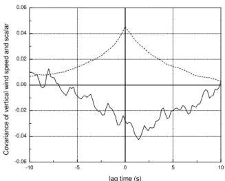
Fig. 3. The lag correlation diagram demonstrates that the covariance (ppb m s−1)for the vertical wind speed and 550◦C (6NOyi) TD-LIF channel (solid line) maximizes at a lagtime of 1.4 s for this half-hour in the late morning of 17 September 2004. The sensible heat covariance (◦C m s−1, divided by 10, dashed line) maximizes at 0 s.
transported in separate lines from the pure zero air to prevent residual NO2from affecting background measurements, and
was introduced as an overflow at the inlet so that it passes through the ovens and sampling lines before being detected. The mixing ratio data were corrected (<5%) for quenching by water (Thornton et al., 2000).
Spikes in NOxcaused by the diesel generator are
occasion-ally observed during periods of light, variable winds, most often at night. Data influenced by spikes were identified and removed by first flagging data points in which NO2or NOy
varied by more than 5 standard deviations from the mean for a given half hour, and then by removing any remaining spikes by hand.
Data from the sonic anemometer were processed by ro-tating the wind vectors for each half hour to ensure that the vertical wind measurements were taken normal to the shear plane (Baldocchi et al., 1988; McMillen, 1988). Data from the sonic anemometer and the LIF system are acquired at the same rate (5 Hz) and on the same computer using programs that run independently. Nonetheless, the data points do not necessarily coincide exactly in time, and may be shifted by <0.2 s. To correct for this problem, we linearly interpolate the LIF data onto the sonic anemometer time stamp prior to flux analysis.
The finite length of tubing between the inlet at the top of the tower and the LIF detection sensor on the ground causes a time lag in measurements taken by the sonic and TD-LIF sys-tems. This time lag is the sum of time taken for a given parcel of air to move past the sonic anemometer and into the inlet,
0 6 12 18 24 Time of Day 0 6 12 18 24 Time of Day 0 6 12 18 24 Time of Day 0 6 12 18 24 -0.01 0.00 0.01 Flux (ppb m s -1) Time of Day HNO3 Alkyl nitrates Peroxy nitrates NO2
Fig. 4. Average fluxes (running mean with standard error, ppb m s−1)of NO2, 6PNs, 6ANs and HNO3from the summer (June–August)
2004.
which is a function of wind speed and distance between the inlet and anemometer, plus the time taken for the air to move from the inlet into the LIF chamber, which is a function of tube length and pumping speed. The pumping speed varied daily with air density, which depends on atmospheric pres-sure and temperature. However, the effect of these variations on lag time was minor (<0.5 s), and did not affect observed fluxes. While the length of sample tubing was roughly the same for each sample line, slight differences in the pinhole size for each sampling line and the arrangement of vacuum tubing from the Roots blower to the LIF chambers caused the pressure in each chamber to be slightly different (between 2.7 and 3.1 Torr), and thus the lagtimes to be different for each channel. This lagtime is accounted for in the EC analysis by shifting the LIF detector data by an appropriate number of data points (lagtime) to align with the sonic data for each of the four channels. The lagtime is determined from plots of the covariance between the sonic and LIF detector at varying lagtimes; a peak in these lagged covariance plots occurs at the lagtime required for the sample air to move through the sample tubing (Fig. 3). As expected, no lagtime is observed between the vertical wind speed and temperature as the ver-tical wind speed and virtual temperature are derived from measurements taken on the same instrument. The maximum covariance observed in a lagged covariance plot for mixing ratio and vertical wind speed is the EC flux. The typical lag-time for a given pump and tubing configuration was deter-mined for each channel, and applied to the dataset; the pump and tubing configuration changed several times throughout the campaign (summer 2003 to summer 2005) due to pump failures. For example, for the summer of 2004, we applied lags of 2.2 s for the 550◦C channel, 2.0 s for the 330 and 180◦C channels, and 2.6 s for the ambient NO2channel.
5 Mixing ratios
NOymixing ratios at UC-BFRS are between 0.5–3 ppb and
exhibit a diurnal trend of increasing mixing ratio with the up-slope wind during the day, maximizing in the late evening, and decreasing when the downslope flows return cleaner
air until late morning (Day, 2003; Dillon et al., 2002). Unlike other rural sites, NOy maxima in the summer are
higher than in the winter (Day, 2003). We attribute this to stronger transport from urban source areas during sum-mer. During the study period, typical NOx mixing
ra-tios range from 0.2 to 1.0 ppb; 6PNs from 0.1 to 1.0 ppb; 6ANs from 0.05 to 0.5 ppb, and HNO30.01 ppb to 1.0 ppb.
The statistics of NOyi mixing ratios are described in
de-tail in Murphy et al. (2006). Ozone mixing ratios ranged from 35 to 70 ppb. Mid-day ozone fluxes are about 0.306– 0.340 ppb m s−1(45–50µ mol m−2h−1)in the summer, and
0.102 ppb m s−1(15µ mol m−2 h−1)in the winter (Kurpius
and Goldstein, 2003). Figure 1 shows the median summer mixing ratios of NO2, 6PNs, 6ANs and HNO3versus time
of day.
6 Eddy covariance fluxes
The EC flux for a given species, Fc, is calculated as the
co-variance between the vertical wind speed and species mixing ratio, Fc= 1 n n X i=1 (wi − ¯w) · (ci− ¯c) (3)
where n is the number of points used for the calculation, wi and ci are instantaneous measurements of vertical wind
speed and mixing ratio, and ¯wand ¯c are the mean vertical wind speed and mixing ratio respectively. A positive flux in-dicates upwards movement of mass from the surface to the atmosphere. Measurements are typically taken for ∼30 min at 5 Hz, which is both long and fast enough to capture all flux-carrying eddies. Fluxes measured by the EC method are valid only if the assumptions behind Taylor’s “frozen flow” hypothesis are met, namely that eddies move past the tower unchanged and in stationary flow (Stull, 1988).
The eddy covariance technique requires that the calculated fluxes do not vary within time-scales of analysis, the station-arity requirement. We tested for stationstation-arity by comparing the 30-min fluxw0c0 30 minto the mean of fluxes calculated from the six consecutive 5-min samples within the half hour,
1E-3 0.01 0.1 1 1E-6 1E-5 1E-4 1E-3 0.01 0.1 1 10 100 spectral density frequency (Hz) b a 1E-3 0.01 0.1 1 1E-3 0.01 0.1 1 10
power spectral density
frequency (Hz)
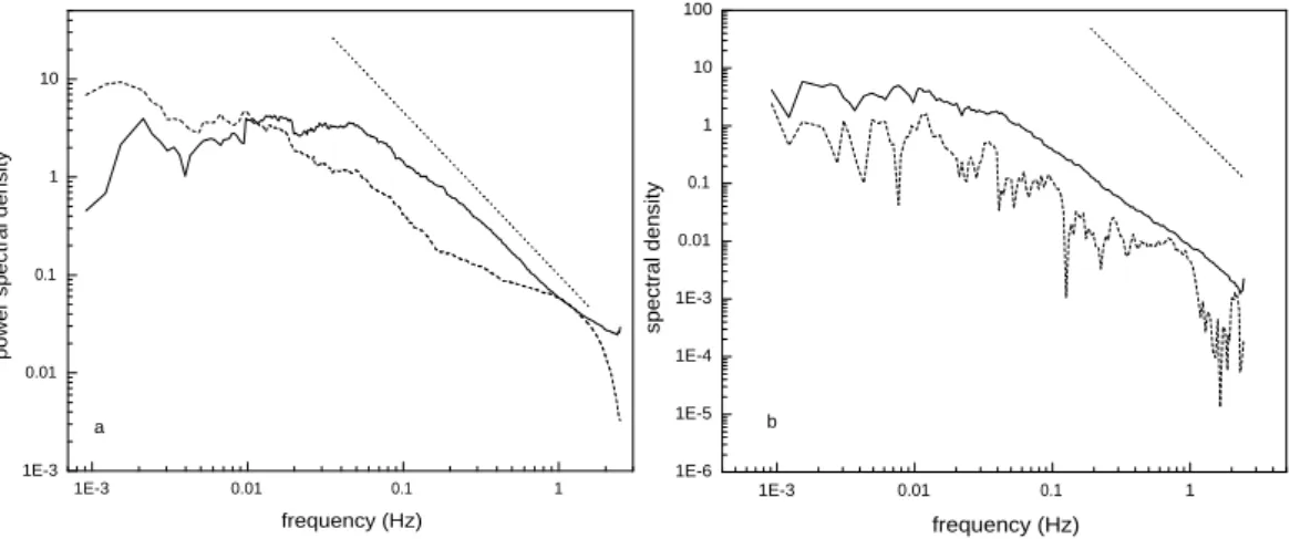
Fig. 5. (a) Power spectrum of vertical wind speed (solid line) and NO2(dashed line) observed during a single half hour in the afternoon
of 17 September 2004; a line with a –5/3 slope indicates the presence of an inertial subrange. (b) Cospectra of vertical wind speed and temperature (solid line) and vertical wind speed and NO2(dashed line) for the same half-hour as (a). A line with a –7/3 slope indicates the
presence of an inertial subrange. Note that the power spectra are binned into 500 evenly spaced intervals along the logarithmic frequency axis; cospectra are similarly binned into 200 intervals.
hw0c0i
5 min. Data for which the ratio of sub-set flux mean to
half-hour mean was not within ±30%(Foken and Wichura, 1996), 0.7<hw 0c0i 5 min hw0c0i 30 min <1.3, (4)
were assumed to be non-stationary. More than 95% of the previously filtered NOy,i data from the winter season
(January–March 2005) were stationary. The sensible heat fluxes are not filtered for spikes due to the nearby genera-tor prior to analysis, and only met the stationarity criterion for 67% during winter 2005. For September 2004, more than 93% of NOyidata not influenced by the generator were
sta-tionary, while 66% of the sensible heat data were stationary. Most of the non-stationary sensible heat fluxes were at times when spikes from the generator were observed.
Nighttime EC CO2fluxes are typically filtered to exclude
data observed in low turbulence regimes, as determined by a threshold friction velocity (u∗)ranging from 0.0 to 0.6 m s−1
(Massman and Lee, 2002). These filters are often applied when CO2fluxes correlate with friction velocity at low u∗,
which should not occur because CO2 fluxes are assumed to
be driven by biological controls, and thus uncorrelated to tur-bulence (Massman and Lee, 2002). However, as the control-ling mechanisms of NO2, 6PNs, 6ANs, and HNO3 fluxes
are poorly understood, there is no clear evidence that the fluxes are biologically determined. Thus we have not re-moved nighttime data that has passed the stationarity test, although nighttime u∗at Blodgett Forest ranged from 0.01 to
0.5 m s−1during September 2004. Future work will analyze the long-term NOyi flux dataset from Blodgett to determine
whether a u∗threshold should be applied.
As fluxes are calculated from the deviations from the mean for a given scalar, a time-varying mean mixing ratio causes spurious fluxes. We used a 10-min running mean to calcu-late the perturbations from the mean for scalar mixing ra-tio and vertical wind speed, c0 and w0. The turbulent flux for a given half hour is the average of the product of these two values, <c0w0>(McMillen, 1988). Sensitivity tests de-termined that the 10-min running mean was long enough to capture trends caused by movement of pollutant plumes and chemical changes; inspection of cospectra (see below) shows that the low frequency eddies that are removed using 10-min means were not important to the total flux. Similar to mixing ratio measurements, fluxes were determined for each of the four channels, and the difference between ad-jacent channels gives the flux for each class. This is theo-retically identical to calculating fluxes by taking the differ-ence between appropriately lagged channels, and calculating the flux for each class of species. The theoretical conclu-sion was borne out in practice, as identical fluxes were calcu-lated either way i.e. F(NO2(T2)–NO2(T1))= F(NO2(T2))–
F(NO2(T1)) where NO2(T )refers to the total NO2observed
at a particular oven temperature. No density corrections are required for the eddy flux measurements as the TD-LIF mea-sures the mixing ratio of a species in the atmosphere rather than the absolute concentration (Webb et al., 1980). All mix-ing ratio and flux analysis programs were written specifically for this instrument.
0.0 0.2 0.4 0.6 0.8 1.0 cu m ul at iv e co nt rib ut io n to fl ux 1E-3 0.01 0.1 1 -0.3 -0.2 -0.1 0.0 0.1 0.2 co sp ec tra l d en si ty frequency (Hz)
Fig. 6. Normalized cumulative contribution to the flux (a) and av-eraged semilogarithmic cospectrum (b) and from all daytime data of 6ANs for 1 August–10 August 2004. The cospectrum is binned into 100 evenly spaced intervals along the frequency axis.
7 Spectral analysis
EC measurements are known to be challenging because of the wide dynamic range in frequency required of the sen-sors. We test the TD-LIF fluxes using a variety of spectral analyses that demonstrate the experimental capabilities. Fig-ures 1 and 3 show mean mixing ratios and fluxes for sum-mer 2004 (June–August). Eddy covariance fluxes are poten-tially subject to underestimation by systematic errors due to 1) time lags between the sonic anemometer and mixing ra-tio measurements and 2) damping of high frequency fluctu-ations. Time lags between mixing ratio and wind measure-ments are accounted for as described above. Damping of high frequency fluctuations may be caused by sensor sepa-ration, smoothing of flows in the sensor lines, and limited sensor response time.
The magnitude of underestimation of fluxes due to the separation distance between the sonic anemometer and the chemical inlet depends on the mean wind speed. The flux un-derestimation can be calculated for lateral (perpendicular to wind direction) and longitudinal (parallel to wind direction) separation using a spectral transfer function (Moore, 1986): Ts(f )=e−9.9f
1.5
(5) where f =n·s
U is the normalized frequency for which the
func-tion is being calculated, n is frequency (Hz), s is the sep-aration distance (m), and is the mean wind speed (m s−1). To evaluate the loss of total flux due to sensor separation, we compared observed cospectra that were corrected by this transfer function to the uncorrected cospectra. The lateral separation between the TD-LIF inlets and sonic anemometer is <0.05 m, and results in a negligible effect on the flux; a 0.05 m separation and mean wind speeds of 0.5, 1.5, 5, and 10 m s−1correspond to underestimation by 1.82, 0.22, 0.03, and 0.01%. The longitudinal separation is 0.3 m. A 0.30 m separation distance and mean wind speeds of 0.5, 1, 2, and 10 m s−1cause underestimation by >99%, 83.3%, 6.2%, and <0.2%. For median daytime windspeeds of 3 m s−1this ef-fect is an error of less than 1%. At night when wind speeds are typically 1 m s−1, this effect can cause significant atten-uation of the flux. However, Moore (1986) points out that this transfer function does not consider wind direction and likely overestimates the loss. We ignore flow distortion due to the inlet and sonic anemometer as the anemometer is faced into the prevailing daytime wind direction. The tilt angle is the angle required to rotate the sonic anemometer vec-tors about the horizontal axis to give a mean vertical wind speed of zero, and provides an indication of flow distortion (Goulden et al., 1996). The tilt angle for 30-min intervals is always less than 10◦ from zero, and indicates only mi-nor flow distortion from either tower shadowing or the in-let set up (McMillen, 1988). The 3.69◦(0.03=standard de-viation from the mean, N=3023) tilt angle for winds in the 200–360◦(SSW–N) direction (1 July 2004 to 30 November 2004), which account for over 75% of daytime winds, has little variability demonstrating negligible flow distortion for daytime winds over the fetch. The variability in tilt angle is greater in the 100–150◦ wind directions (–1.3◦, σ =0.06, N=2821), demonstrating that passing through the tower (NE-SE winds) affects turbulence. Nighttime fluxes will be more significantly impacted, as only ∼35% of the winds originate in the 200–360◦direction. As the variance in tilt angle in the prevailing wind direction is relatively small, the inlet design likely does not cause significant flow distortion.
When fluids pass through long sample tubes, the high fre-quency fluctuations are dampened by smearing due to the dif-ferent speeds traveled by fluctuations being carried at differ-ent frequencies, or spectral attenuation (Lenschow and Rau-pach, 1991). We calculate the half-power fluctuation damp-ing frequency of the sample tubdamp-ing (1/8”i.d.) accorddamp-ing to
1E-3 0.01 0.1 1 1E-8 1E-7 1E-6 1E-5 1E-4 1E-3 0.01 0.1 1 10 100 po w er s pe ct ra l d en si ty frequency (Hz) b a 1E-3 0.01 0.1 1 1E-7 1E-6 1E-5 1E-4 1E-3 0.01 0.1 1 co sp ec tra l p ow er d en si ty frequency (Hz)
Fig. 7. Unsmoothed power spectra (a) of 6NOyi (black) and instrument noise (grey) for this channel, and cospectrum (b) of 6NOyiand
vertical wind speed for a single half hour; stars are at 0.04, 0.08, 0.12, and 0.16 Hz marking the frequency and harmonics of the etalon chop cycle.
Lenschow and Raupach (1991); this is the frequency at which half the spectral power is lost due to attenuation. The half-power damping frequency is ∼6 Hz for our system. Damping at this frequency will result in minimal attenuation of NOyi
fluxes as cospectra show that most of the NOyiflux is carried
by turbulence occurring on significantly slower timescales. A spectral correction may be applied to data to account for this dampening effect on observable fluctuations. One com-monly used correction technique is to apply a transfer func-tion to the cospectra to determine the fracfunc-tional error of the measured flux, and to account for signal loss (Massman, 1991; Moore, 1986). Application of Massman’s transfer function to typical cospectra from our dataset demonstrates that under most circumstances <2% of the flux is lost due to spectral attenuation. In rare circumstances when the cal-culated lagtimes indicate a slower flow through the tubing, losses as high as 7% are calculated.
Power spectra of both the observed vertical wind speed and LIF mixing ratio data are level at the low frequencies (0.02 Hz), showing that the measurement interval of 30 min is long enough to capture the low frequency eddies that carry flux (Fig. 5a). The spectrum for only one channel is pre-sented because all four channels have very similar spectra, as expected for identical inlet configurations and detection tech-niques. The power spectra have (frequency)−5/3behavior for frequencies between 0.02 and 0.8 Hz, indicative of the iner-tial subrange and demonstrating that the TD-LIF sensitivity is adequate to measure mixing ratio perturbations due to tur-bulence (Anderson et al., 1986). At frequencies greater than ∼1 Hz the mixing ratio power spectra become noise limited as indicated by the rapid fall off in spectral density.
Cospectra of vertical wind speed and temperature and ver-tical wind speed and mixing ratio both show the same slopes, and both deviate from the expected (frequency)−7/3slope in the same way (Fig. 5b). This behavior is characteristic of the inertial subrange between 0.01–0.8 Hz. Again, all four
chan-nels produce similar logarithmic cospectra. The slopes for both TD-LIF and sonic anemometer cospectra are more shal-low than the –7/3 slope expected from Komolgorov theory, which can not be due to spectral attenuation, as this should not occur in the sensible heat cospectra. The –7/3 slope is predicted from dimensional analysis, and deviations are not unprecedented. In long-term studies of turbulence spectra over two mixed hardwood forests, Su et al. (2004) observed turbulence spectra with shallower slopes in the inertial sub-range than the expected. Blanken et al. (1998) similarly ob-served cospectral slopes in the inertial subrange less than the-oretically expected for fluxes of sensible heat, water and CO2
both above and below a boreal aspen forest. The shallow cospectra slopes observed in this study suggest that the cas-cade of energy transfer from larger to smaller eddies in the in-ertial subrange occurs with a power law smaller than the -7/3 suggested by dimensional analysis. The cospectra on a semi-logarithmic scale (Fig. 6) further demonstrate that the main contributions to flux are from eddies in the 0.01 to 0.5 Hz frequency range (corresponding to 6–300 m horizontally for a 3 m s−1wind) (Anderson et al., 1986; Kaimal et al., 1972). This frequency range is similar to the 0.005 to 0.5 Hz range observed for NOy by Munger et al. (1996), and confirms
that the TD-LIF time response is adequate. The structure observed within the TD-LIF cospectra can be removed by averaging data in larger frequency bins, but is potentially in-dicative of complex process controlling NOyifluxes, and was
thus preserved in Fig. 5. The data also confirm that measure-ments with characteristic time constants significantly shorter than the maximum 0.6 s TD-LIF time constant would have been of limited additional benefit. Loss of flux signal from the instrument time constant can be approximated as:
Fm
Ft
= 1
(1 + 2πfmτ )
1E-3 0.01 0.1 1 -0.010 -0.008 -0.006 -0.004 -0.002 0.000 0.002 0.004 0.006 0.008 0.010 co sp ec tra l d en si ty (in st ru m en t n oi se , v er tic al w in d sp ee d) frequency (Hz)
Fig. 8. Cospectrum of instrument noise (zero air measurements) and vertical wind speed, demonstrating the lack of covariance and thus minimal impact of noise on observed fluxes. This cospectrum is binned into 94 evenly spaced intervals along the logarithmic fre-quency axis.
where Fm is the observed flux, Ft is the true flux, fm is
the frequency at which the frequency-multiplied cospectrum maximizes, and τ is the first-order response time of the sen-sor (Horst, 1997). For fmof 0.01 Hz and τ of 0.6 s, the
un-derestimation is 3.6% for the HNO3flux. As these are
con-servative estimates of fm and τ , we do not correct for this
underestimation in the fluxes presented in Fig. 4.
To test for interferences and prevent drift of the laser fre-quency, the TD-LIF measurement algorithm alternates the laser frequency on and off the NO2resonance in a 25 s cycle.
However, imperfections in the instrument calibration at the on and off resonance frequencies will introduce fluctuations at 25 s (0.04 Hz), which could potentially covary with fluc-tuations in the vertical wind speed, causing spurious fluxes. The power spectra (e.g. Fig. 7a) show a clear, narrow peak at 0.04 Hz, as well as the harmonics of this signal at 0.08, 0.12, and 0.16 Hz (marked with stars). The cospectra of mix-ing ratio and vertical wind speed (Fig. 7b) still have peaks at 0.04 Hz and its harmonics, but they are dampened because the chop cycle is independent of fluctuations in the verti-cal wind speed. The potential effect of the chop cycle on fluxes was quantified by integrating the area under the semi-log cospectrum in the frequency regions affected by the chop cycle and determined to be negligible (<1%).
The LIF-vertical wind speed cospectra are less coherent than the sensible heat cospectra derived solely from the sonic anemometer (Fig. 5b). The high-frequency (≥1 Hz) noise is possibly due to higher instrument noise in the LIF detec-tor than the sonic anemometer. The variations at lower fre-quencies for the mixing ratio cospectra are more likely due to chemical reactions and the fact that production and depo-sition of certain species is inhomogeneous within the fetch,
causing varying mixing ratios in the horizontal plane, thus af-fecting observed fluxes and cospectra (Delany et al., 1986). Future studies will include a more thorough analysis of these variations.
Instrument noise may correlate with vertical wind speed resulting in a spurious flux, contributing to uncertainty in the observed scalar flux. We determine this uncertainty both the-oretically and experimentally. The contribution to flux vari-ance due to instrument noise, σ2inst(F ; T ), can be written as
σinst2 (F ; T ) = σ
2
wσn21t
T (7)
where σ2wand σ2nare the variance in vertical wind speed (m2 s−2)and instrument noise (ppb2)respectively, 1t is the sam-pling interval (0.2 s for 5 Hz measurements), and T is the averaging time (s)(Lenschow and Kristensen, 1985; Ritter et al., 1990). As the instrument noise is dominated by shot noise, the variance in instrument noise can be calculated for each half hour sampling interval as the square root of the to-tal number of photon counts, converted to mixing ratio units by the appropriate calibration constant. The photon counts vary with scalar mixing ratio and laser alignment within each White cell. The calculated contribution to error in the mea-sured fluxes from instrument counting noise is calculated as the square root of σ2inst. For example, for typical noon-time σ2w of 0.7 m2 s−2 and instrument shot noise of 0.01 ppb, the σ2inst(F ; T ) is 7.8×10⁻⁹ ppb2 m2 s−2, causing an un-certainty of 8.8×10⁻⁵ppb m s−1(0.013 µmolm−2hr−1)for a half hour of 5 Hz data. On a typical day the average un-certainty in the flux ranged from 1.4×10⁻⁶ppb m s−1for the 550◦C channel to 2.9× 10⁻⁵ppb m s−1for NO2. These
cal-culated contributions to error in the measured fluxes are or-ders of magnitude less than the measurements. The contri-bution to flux uncertainty for 6PNs, 6ANs and HNO3 is
calculated by propagation of the contributions from adjacent channels. For example, the error for fluxes centered around noon of 10 September 2004, a typical summer day, are calcu-lated to be 7.0×10⁻⁵, 3.7×10⁻⁵ and 1.4×10⁻⁵ ppb m s−1 for 6PNs, 6ANs, and HNO3, respectively.
Zero-air measurements provide experimental validation that TD-LIF fluxes are not dominated by instrument noise. Zero air was flowed into the inlet continuously for ∼30 min in the morning of 10 September 2004, and the observed LIF signals in each channel were combined with sonic anemome-ter data to calculate a zero-air flux. Because TD-LIF mea-surement rely on differences between the channels there might be additional contributions to the error budget of a measurement associated with imperfect subtraction that are not captured by these zero air fluxes. However we have found no evidence for such effects. The zero air fluxes are single-point measurements of instrument noise to flux. Because the variance is the integral of a power spectrum, comparison of the power spectra of a half-hour of zero air (Fig. 7a, grey) to a half hour of 6NOyi (Fig. 7a, black)
0 6 12 18 24 Time of Day 0 6 12 18 Time of Day 0 6 12 18 Time of Day 0 6 12 18 -0.01 0.00 0.01 Fl ux (p pb m s -1) Time of Day 0.0 0.1 0.2 0.3 0.4 0.5 0.6 M ix in g ra tio (p pb )
NO
2 ΣPeroxy nitrates
ΣAlkyl nitrates
HNO
3Fig. 9. (a–d). Average mixing ratios (ppb, upper panels) and fluxes (running mean with standard error, ppb m s−1, lower panels) of HNO3,
6alkyl nitrates, 6peroxy nitrates, and NO2for winter (1 January–31 March 2005).
demonstrates that the variance in measured 6NOyi is
min-imally affected by variance in instrument noise. The cospec-trum of inscospec-trument noise (Fig. 8) is completely flat with a maximum amplitude of 0.008 ppb m s−1independent of fre-quency, compared to typical mixing ratio fluxes (Fig. 5b) which exhibit an inertial sub-range. We calculated fluxes from the half-hour of measurements of zero-air with 30 min intervals of vertical wind speed data following protocols identical to our EC flux calculations for atmospheric data. The maximum and minimum noise flux for 10 September 2004 were 3.8×10⁻⁴and 1.3×10⁻⁶ppb m s−1for the 550◦C channel, and 4.6×10⁻³and 5.9×10⁻⁶ppb m s−1for the
am-bient NO2channel. For the differences between channels we
observe maximum zero air fluxes of 6.3×10⁻⁵, 7.5×10⁻³,
and 1.2×10⁻³ppb m s−1and minimum fluxes of 6.3×10⁻⁵, 5.8×10⁻⁶, and 6.9×10⁻⁷ppb m s−1for 6PNs, 6ANs, and HNO3. For reasons we cannot fully explain, these
measure-ments are an order of magnitude larger than the error calcu-lated using Eq. (7), though they are still small compared to the measured fluxes. As an example, Table 1 compares ob-served fluxes with theoretical and experimental estimates of noise for the half-hour at noon on 10 September 2004.
These zero fluxes can be used to estimate a minimum ob-servable flux using the TD-LIF method of subtracting ad-jacent channels. As fluxes for 6PNs, 6ANs, and HNO3
are calculated as a difference in fluxes of adjacent channels (Fdiff), we can consider the flux measurement sensitivity due
to instrument noise similarly to the above calculations of the random component of uncertainties and sensitivities in mix-ing ratio data:
Fdiff=FA−FB±12F a+1
2
F b)
1/2 (8)
For 10 September 2004, with a S/N=2=FA–
FB/(12F a+12F b)1/2, where 1F a and 1F b=1.6×10⁻⁵
and 1.1 ×10⁻⁴ppb m s−1 for the HNO3 channel, we
cal-culate that |FA–FB| 2.2×10⁻⁴ppb m s−1 (0.032 µmol m−2
hr−1)will have S/N >2. Similarly, the minimum observable flux is 2.2×10⁻⁴ and 6.0×10⁻⁴ppb m s−1 for 6ANs and 6PNs respectively. While it is difficult to generalize this estimate of a detection limit because it depends both on the instrument sensitivity and on the variance of the vertical winds, we do find that daytime fluxes are almost always a factor of 10–100 larger than the uncertainty estimated from the zero air measurement, and that nighttime fluxes when u∗<0.1 m s−1may sometimes have signal to noise less than
2.
8 Patterns in the fluxes
The fluxes and mixing ratios observed at Blodgett Forest rep-resent a large and complex that dataset will be discussed in detail in future manuscripts.
The mean winter fluxes (Fig. 9) demonstrate the poten-tial of the TD-LIF method when coupled to EC. Winter-time 6NOyi fluxes are dominated by midday deposition of
6peroxy nitrates, 6alkyl nitrates and HNO3, while NO2
ex-hibits a variable, if slightly upward, flux. The net downward flux of 6ANs and 6PNs flux is a sign of the potentially im-portant role of deposition of these organic nitrogen species to the forest ecosystem during winter. Upward NO2fluxes may
be due to a combination of several processes. As the NO2
Table 1. Errors in eddy covariance fluxes from TD-LIF instrument noise from half-hour centered around noon, 10 September 2004.
Channel Observed Flux
(ppb m s−1)
Theoretical noise (ppb m s−1) (relative error)
Zero air flux (ppb m s−1) (relative error) 550◦C (6NOyi) 0.0184 3.44×10⁻⁶ (0.02%) 1.50×10⁻⁵ (0.08%) 330◦C (6ANs + 6PNs + NO2) .0173 1.40×10⁻⁵ (0.08%) 3.38×10⁻⁴ (1.95%) 180◦C (NO2+6PNs) 0.0467 3.37×10⁻⁵ (0.07%) –1.9×10⁻³ (4.1%) Ambient (NO2) 0.0196 6.17×10⁻⁵ (0.31%) 1.8×10⁻³ (9.2%)
within the ecosystem to release NO2, as observed on the leaf
scale for tropical plants (Sparks et al., 2001). As the ground was covered by snow during the winter, a direct release of NO2 as a result of snow photochemistry could also cause
emission (Domine and Shepson, 2002). A third mechanism potentially responsible for the upward NO2 fluxes is
emis-sion of NO, either from plants (Wildt et al., 1997) or snow (Domine and Shepson, 2002), followed by reaction with O3
in the canopy, resulting in a net observed upward flux. Fluxes of all species are significantly smaller at nighttime than day-time, likely due to the low turbulence (u∗<0.17 m s−1)and
significant attenuation. Further, as the nighttime wind direc-tion is in the opposite direcdirec-tion from the sonic anemometer, air may have to pass through the tower before reaching the in-let and anemometer, causing perturbations to the turbulence and removing the stickier HNO3and hydroxyl-alkyl nitrates.
During the winter, mixing ratios of 6NOyare lower than
in the summer (Figs. 1, 9). Regional winds in the winter are weaker, preventing the Sacramento air plume from reaching Blodgett Forest much of the time. The variability in mixing ratio likely contributes to the variability in observed deposi-tion. By normalizing the flux by mixing ratio, we can obtain the deposition velocity, Vdep:
Vdep=
−F
C (9)
where F is the flux and C is the mixing ratio. The Vdepis
typ-ically thought of as the result of a molecule passing through a series of resistances between the atmosphere and ecosystem, Vdep=
1 Ra+Rb+Rc
(10) where Ra is the aerodynamic resistance, Rb is the
lami-nar boundary-layer resistance and Rc is the canopy
resis-tance. The observed Vdep derived from flux and mixing
ra-tio measurements can be compared to the theoretical max-imum Vdep, or Vmax, which assumes that the gas is always
absorbed by the ecosystem surfaces (i.e. Rc=0). To
cal-culate a Vmax, we estimated Ra and Rb by the Dry
De-position Inferential Method from observed windspeeds and
u∗(Hicks et al., 1987). The average summer Vmaxwas 0.042
to 0.047 m s−1 in the daytime, and 0.0 to 0.008 m s−1 at night. The average winter Vmaxshowed significantly more
variability, ranging from 0.015 to 0.044 m s−1in the daytime, and between 0 and 0.015 m s−1at night. The median Vdepfor
HNO3 during winter afternoons between 11:00–13:00 PST
was 0.025 m s−1, and 80% of the data fall between Vdep of
–0.012 and 0.082 m s−1. For 6ANs the median Vdep was
0.021 m s−1, and 80% fell in the range 0.013 to 0.18 m s−1, while for 6PNs the median Vdepwas 0.0084 m s−1, and the
80% range is –0.0057 to 0.063 m s−1. The observed V depfor
all species measured by TD-LIF were significantly less, sug-gesting that either the resistance model overestimates the re-sistances, or that canopy resistances were significant, which is likely the case for all species other than HNO3. Further,
observed HNO3and 6 ANs fluxes may be affected by
semi-volatile components. The contribution of ammonium nitrate aerosol (NH4NO3) is expected to be minor at Blodgett Forest
as there are no local NH3sources, and any NH3or NH4NO3
originating from the agricultural region of the Central Valley are expected to have deposited by the time the air mass has reached Blodgett Forest. Observations at Whitaker Forest in the western Sierra Nevada, closer to agricultural sources than Blodgett Forest, measured NH4NO3mixing ratios less
than 0.15 ppb during the summer Bytnerowicz and Riechers, 1995). Particulate NH4NO3 is expected to deposit to
sur-faces, though with a slower Vdepthan gas-phase HNO3due to
an increased aerodynamic resistance; the resulting effect on observed TD-LIF HNO3fluxes would be diminished
deposi-tion rates, and thus a smaller Vdep. To our knowledge, there
are no specific studies of particulate alkyl nitrates in forest regions, though aerosol measurements by Allan et al. (2006) over a boreal forest suggested that organic nitrates may have a particulate component that would, if present, reduce the observed Vdep.
The net exchange of 6NOyi over a given period can be
derived by integrating the total flux over the time period of interest. Unfortunately, generator failures and instrumental problems at Blodgett Forest occurred throughout the winter,
Table 2. Summary of errors affecting TD-LIF eddy covariance fluxes, with conservative estimates of relative contribution to flux.
Source of Error Bias Relative error
(1 m/s mean wind
speed)
Relative error
(5 m/s mean wind
speed)
Error analysis reference
Sensor separation, lateral Underestimate <0.43% <0.03% Moore, 1986
Sensor separation, longitudinal Underestimate <20.2 <0.25% Moore, 1986
Spectral attenuation Underestimate <7% (typically, <2%) Lenschow & Raupach, 1991
Instrument time response Underestimate <3.6% Horst, 1997
Chop cycle None <1% this work
Instrument noise None <2%a Lenschow & Kristensen, 1985,
Ritter et al. 1990
Instrument noise None <15%b this work
a=For lowest instrument sensitivities kept in this dataset b=For typical results by channel, see Table 1
and resulted in a patchy dataset that included only a third of the winter days (1 January 2005–31 March 2005). To de-termine the net exchange, we integrated the average win-ter diurnal cycle of 6NOyi fluxes, and multiplied by 90
days. Assuming that the median winter cycle adequately represents the winter exchange, Blodgett Forest experiences 0.102 kg N ha−1 dry 6NOy deposition in the winter. No
previous measurements of dry deposition have been made at UC-BFRS, though estimates of summer deposition fluxes to Ponderosa pines at Whitaker’s Forest, which is south of UC-BFRS, from a foliage rinsing technique estimated an-nual dry deposition (NO−3 + NH+4, gas + particle) of 1.0– 1.5 kgN ha−1(Bytnerowicz and Riechers, 1995). Other stud-ies suggest the Sierra Nevada receives an average of 1.7 kgN ha−1yr−1wet (NO−3 + NH+4)deposition. (Bytnerowicz and Fenn, 1996). Measurements at Lake Tahoe, which is higher in elevation and further east than Blodgett, indicate summer-time dry deposition (HNO3(g)+ NH3(g)+ NH4NO3(p))
rang-ing from 1.2–8.6 kg N ha−1 yr−1 for the summer and fall, versus wet deposition (NO−3 + NH+4), which ranges from 1.7 to 2.9 kg N ha−1yr−1(Tarnay et al., 2001). The TD-LIF-derived estimate of dry deposition of NOyi species during
the winter at Blodgett Forest is lower than total N deposition measurements elsewhere in the Sierra Nevada, likely because of higher HNO3mixing ratios in the summer and high HNO3
mixing ratios closer to direct NOx sources in California’s
Central Valley or from tourism within the Lake Tahoe basin. While the TD-LIF derived dry deposition estimate does not include contributions of reduced N, these compounds are ex-pected to be minor at Blodgett Forest, and should not con-tribute strongly to a deposition flux.
Mean summer fluxes (Fig. 4) are characterized by upward fluxes in NO2, 6PNs, and HNO3, and downward fluxes of
6ANs. The net upward NO2, 6PNs and HNO3fluxes
sug-gest that within canopy chemistry competes with deposition for these reactive nitrogen oxides. The NO2 observations
are consistent with previous studies of O3at Blodgett
For-est, which indicate chemical fluxes of O3 due to reactions
with NO emitted from soil microbial processes (Kurpius and Goldstein, 2003). The upward fluxes of 6PNs and HNO3 are likely due to within-canopy production
follow-ing reaction of NO2 with OH and RC(O)O2 radicals
pro-duced during VOC oxidation. OH mixing ratios within the canopy at Blodgett Forest have been estimated as between 0.8–3×10⁷molecules cm−3as a result of oxidation of VOCs
by O3(Goldstein et al., 2004). We speculate that these high
OH mixing ratios are adequate to produce enough within-canopy HNO3 to affect the observed fluxes. Similarly the
OH may affect 6ANs and 6PNs through various chemical cycles. This mechanism, and some possible alternatives that were incapable of describing the data, are presented in more detailed in Farmer and Cohen (2006)2. These data give a hint of the enormous potential for mechanistic studies of factors controlling N fluxes and processing of N by and within forest canopies that EC with TD-LIF provides.
9 Conclusions
We describe the application of TD-LIF for measuring eddy covariance fluxes of NO2, 6PNs, 6ANs, and HNO3.
Spec-tral analysis of the data demonstrate that the TD-LIF mea-surements have the necessary time response and sensitivity to measure fluxes by eddy covariance, and that internal diag-nostics and line locking procedures do not compromise the flux measurements. We evaluated sources of random error and possible biases in TD-LIF flux measurements; these are summarized in Table 2. Sensor separation, spectral attenua-tion in sample tubing, and instrument time response combine
2Farmer, D. K. and Cohen, R. C.: Forest nitrogen oxide
emis-sions: Evidence for rapid chemistry within the canopy, submitted, 2006.
to produce a bias of less than 3.5% underestimation of day-time fluxes under typical atmospheric conditions. The laser chop cycle may contribute as much as a 1% random error. Both theoretical and experimental treatments of the contri-bution of instrument noise to flux error demonstrate that ob-served fluxes are not dominated by instrument noise. Zero air fluxes suggest that instrument noise typically contributes a random error of much less than 10% of the observed fluxes. Typical measurement errors in eddy covariance CO2 fluxes
range from <7% during the day to <12% at night (Baldoc-chi, 2003 and references therein). Thus the major source of error in individual half-hour eddy covariance measurements of both CO2and TD-LIF NOyiis likely the natural
variabil-ity in turbulence, likely between 10 and 20% (Wesely and Hart, 1985). This short-term error in flux measurements is reduced by applying longer-term averages of daily, weekly, or monthly fluxes (Baldocchi, 2003; Goulden et al., 1996).
Initial observations at Blodgett Forest demonstrate that TD-LIF has the potential to shed light on the complexity of ecosystem-level exchange of the reactive nitrogen oxides. Winter fluxes at Blodgett Forest are dominated by deposition of HNO3, 6ANs and 6PNs. Within-canopy chemistry and
the more complex factors controlling summer fluxes will be the subject of further study.
Acknowledgements. This research was supported by the NSF
Atmospheric Chemistry Program under grant ATM-0138669. We gratefully acknowledge D. Day, E. Conlisk and I. Faloona for their contributions in the early stages of this project. Special thanks to the staff at UC-BFRS, in particular S. and D. Rambeau, for exceptional logistical support.
Edited by: W. E. Asher
References
Aber, J., McDowell, W., Nadelhoffer, K., Magill, A., Berntson, G., Kamakea, M., McNulty, S., Currie, W., Rustad, L., and Fernan-dez, I.: Nitrogen saturation in temperate forest ecosystems: Hy-potheses revisited, Biosci., 48, 921–934, 1998.
Allan, J. D., Alfarra, M. R., Bower, K. N., Coe, H., Jayne, J. T., Worsnop, D. R., Aalto, P. P., Kulmala, M., Hyotylainen, T., Cav-alli, F., and Laaksonen, A.: Size and composition measurements of background aerosol and new particle growth in a Finnish forest during QUEST 2 using an Aerodyne Aerosol Mass Spectrometer, Atmo. Chem. Phys., 6, 315–327, 2006.
Anderson, D. E., Verma, S. B., Clement, R. J., Baldocchi, D. D., and Matt, D. R.: Turbulence spectra of CO2, water vapor,
tempera-ture, and velocity over a deciduous forest, Agr. Forest Meteorol., 38, 81–99, 1986.
Baldocchi, D. D., Hicks, B. B., and Meyers, T. P.: Measuring biosphere-atmosphere exchanges of biologically related gases with micrometeorological methods, Ecology, 69, 1331–1340, 1988.
Baldocchi, D. D.: Assessing the eddy covariance technique for evaluating carbon dioxide exchange rates of ecosystems: past, present and future, Glob. Change Biol., 9, 479–492, 2003. Bertram, T. H. and Cohen, R. C.: A prototype instrument for the
detection of semi-volatile organic and inorganic nitrate aerosol, Eos Trans. AGU, 84, 2003.
Bertram, T. H., Heckel, A., Richter, A., Burrows, J. P., and Cohen, R. C.: Satellite measurements of daily variations in soil NOx emissions, Geophys. Res. Lett., 32, L24812,
doi:10.1029/2005GL024640, 2005.
Blanken, P. D., Black, T. A., Neumann, H. H., Den Hartog, G., Yang, P. C., Nesic, Z., Staebler, R., Chen, W., and Novak, M. D.: Turbulent flux measurements above and below the overstory of a boreal aspen forest, Bound-Lay Meteorol., 89, 109–140, 1998. Bobbink, R., Heil, G. W., and Raessen, M. B. A. G.:
Atmo-spheric Deposition and Canopy Exchange Processes in Heath-land Ecosystems, Environmental Pollution, 75, 29–37, 1992. Bragazza, L. and Limpens, J.: Dissolved organic nitrogen
dominates in European bogs under increasing atmospheric N deposition, Global Biogeochem. Cycles, 18, GB4018, doi:10.1029/2004GB002267, 2004.
Brost, R., Delany, A., and Huebert, B.: Numerical modeling of con-centrations and fluxes of HNO3, NH3and NH4NO3near the
sur-face, J. Geophys. Res., 93, 7137–7152, 1988.
Bytnerowicz, A. and Riechers, G.: Nitrogenous Air-Pollutants in a Mixed-Conifer Stand of the Western Sierra-Nevada, California, Atmos. Environ., 29, 1369–1377, 1995.
Bytnerowicz, A. and Fenn, M. E.: Nitrogen deposition in California forests: A review, Environmental Pollution, 92, 127–146, 1996. Cleary, P. A., Murphy, J. G., Wooldridge, P. J., Day, D. A., Millet,
D. B., McKay, M., Goldstein, A. H., and Cohen, R. C.: Observa-tions of total alkyl nitrates within the Sacramento Urban Plume, Atmos. Chem. Phys. Discuss., 5, 2005.
Dabberdt, W. F., Lenschow, D. H., Horst, T. W., Zimmerman, P. R., Oncley, S. P., and Delany, A. C.: Atmosphere-surface exchange measurements, Sci., 260, 1472–1481, 1993.
Davidson, E. A. and Kingerlee, W.: A global inventory of nitric oxide emissions from soils, Nutrient Cycling in Agroecosystems, 49, 37–50, 1997.
Day, D. A., Wooldridge, P. J., Dillon, M. B., Thornton, J. A., and Cohen, R. C.: A thermal dissociation laser-induced fluo-rescence instrument for in situ detection of NO2, peroxy ni-trates, alkyl nini-trates, and HNO3, J. Geophys. Res., 107, 4046,
doi:10.1029/2001JD000779, 2002.
Day, D. A., Dillon, M. B., Wooldridge, P. J., Thornton, J. A., Rosen, R. S., Wood, E. C., and Cohen, R. C.: On alkyl ni-trates, O3, and the “missing NOy”, J. Geophys. Res., 108, 4501, doi:10.1029/2003JD003685, 2003.
Delany, A. C., Fitzjarrald, D. R., Lenschow, D. H., Pearson Jr., R., Wendel, G. J., and Woodruff, B.: Direct measurements of nitro-gen oxides and ozone fluxes over grassland, J. Atmos. Chem., 4, 429–444, 1986.
Dillon, M. B., Lamanna, M. S., Schade, G. W., Goldstein, A. H., and Cohen, R. C.: Chemical evolution of the Sacramento urban plume: Transport and oxidation, J. Geophys. Res., 107, 4045, doi:10.1029/2001JD000969, 2002.
Domine, F. and Shepson, P. B.: Air-snow interactions and atmo-spheric chemistry, Sci., 297, 1506–1510, 2002.