HAL Id: inria-00590040
https://hal.inria.fr/inria-00590040
Submitted on 10 Aug 2011HAL is a multi-disciplinary open access
archive for the deposit and dissemination of sci-entific research documents, whether they are pub-lished or not. The documents may come from teaching and research institutions in France or abroad, or from public or private research centers.
L’archive ouverte pluridisciplinaire HAL, est destinée au dépôt et à la diffusion de documents scientifiques de niveau recherche, publiés ou non, émanant des établissements d’enseignement et de recherche français ou étrangers, des laboratoires publics ou privés.
Smooth Curve Extraction by Mean Field Annealing
Laurent Herault, Radu Horaud
To cite this version:
Laurent Herault, Radu Horaud. Smooth Curve Extraction by Mean Field Annealing. Annals of Math-ematics and Artificial Intelligence, Springer Verlag, 1995, 13 (3-4), pp.281–300. �10.1007/BF01530832�. �inria-00590040�
Annals of Mathematics and Artificial Intelligence 13(1995) 281–300
Smooth Curve Extraction by Mean Field Annealing
∗Laurent H´erault
LETI (CEA-Technologies Avanc´ees)
D´epartement Syst`emes
CENG, 17 avenue des Martyrs
38054 Grenoble FRANCE
Radu Horaud
LIFIA–IMAG
46, avenue F´elix Viallet
38031 Grenoble FRANCE
Abstract
In this paper we attack the figure-ground discrimination problem from a combinatorial optimization perspective. In general the solutions proposed in the past solved this problem only partially: either the mathematical model encoding the figure-ground problem was too simple or the optimization methods that were used were not efficient enough or they could not guarantee to find the global minimum of the cost function describing the figure-ground model. The method that we devised and which is described in this paper is tailored around the following contributions. First, we suggest a mathematical model encoding the figure-ground discrimination problem that makes explicit a definition of shape (or figure) based on cocircularity, smoothness, proximity, and contrast. This model consists of building a cost function on the basis of image element interactions. Moreover, this cost function fits the constraints of a interacting spin system which in turn is a well suited physical model to solve hard combinatorial optimization problems. Second, we suggest a combinatorial optimization method for solving the figure-ground problem, namely mean field annealing which combines mean field approximation and annealing. Mean field annealing may well be viewed as a deterministic approximation of stochastic methods such as simulated annealing. We describe in detail the theoretical bases of this method, derive a computational model, and provide a practical algorithm. Finally, some experimental results are shown both with synthetic and real images.
I
Introduction
The problem of separating figure from ground is a central one in computer vision. One aspect of this problem is the problem of separating shape from noise. Two-dimensional shapes are the input data of high-level visual processes such as recognition. In order to maintain the complexity of recognition as low as possible it is important to determine at an early level what is shape and
∗This research has been sponsored in part by “Commissariat `a l’Energie Atomique,” and in part by the ORASIS
what is noise. Therefore one needs a definition of shape, a definition of noise, and a process that takes as input image elements and separates them into shape and noise.
In this paper we suggest an approach whose goal is twofold: (i) it groups image elements that are likely to belong to the same (locally circular) shape while (ii) noisy image elements are eliminated. More precisely, the method that we devised builds a cost function over the entire image. This cost function sums up image element interactions and it has two terms, i.e., the first enforces the grouping of image elements into shapes and the second enforces noise elimination. Therefore the shape/noise discrimination problem becomes a combinatorial optimization problem, namely the problem of finding the global minimum for the cost function just described. In theory, the problem can be solved by any combinatorial optimization algorithm that is guaranteed to converge towards the global minimum of the cost function.
In practice, we implemented three combinatorial optimization methods: simulated annealing (SA), mean field annealing (MFA), and microcanonical annealing (MCA) [8]. Here we concentrate on mean field annealing.
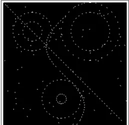
Figure 1: A synthetic image with 1250 ele-ments. Circles, a straight line, and a sinusoid are plunged into randomly generated elements.
Figure 2: The result of applying mean field an-nealing to the synthetic image. The elements shown on this figure were labelled “shape”. The figure-ground or shape/noise separation problem is best illustrated by an example. Figure 1 shows a synthetic image. In this image some elements belong to such shapes as circles, a straight line, and a sinusoid while some other elements are noise. Two independent sequences of random numbers were used to generate this noise: One sequence for the position in the image and another sequence for the orientation. This image has a total of 1250 elements. Figure 2 shows the result obtained with mean field annealing. This image contains 309 elements that were labelled “shape” by this algorithm. Notice that edges belonging to such generic shapes as circles, straight lines, and sinusoids were correctly labelled as shapes while most of the noise was thrown out. Also, there are a number of isolated noise edgels that were incorrectly labelled shape: these isolated edgels can be easily eliminated by some straightforward post-processing.
II
Background and contribution
The interest for shape/noise separation stems from Gestalt psychologists’ figure-ground demons-trations [12]: certain image elements are organized to produce an emergent figure. Ever since the figure-ground discrimination problem has been seen as a side effect of feature grouping. The prerequisite of any method is the extraction from the raw data of the image elements that are either to be grouped or to be thrown out. Edge detection is in general first performed. Grouping edges is done on the basis of their connectivity or by using a clustering technique. Noise is eliminated by thresholding.
The connectivity analysis produces edge chains which are further fitted with piecewise analytic curves (lines, conics, splines, etc.). The clustering technique maps image edges into a parameter space and such a parameter space is associated with each curve type: this is the well known Hough transform. The problem of finding curves in the image is equivalent to a clustering problem in parameter space. With this technique, curves can be detected even if their constituting edges are not connected in the image. There are two major problems with the techniques just described:
1. One has to specify analytically the type of curve or curves that are to be sought in the image and this is done at a low-level of the visual process. At an early stage of an image interpretation system one may just want to know whether a set of edges form a shape or not, without any specific knowledge about the analytic curve that may fit this shape. For example, recognition of object prototypes needs such a vague description.
2. The notion of noise is not clearly specified with respect to the notion of shape. Hence noise elimination takes the form of adhoc methods. For example, edges associated with low contrast are usually thrown out. There are many examples that tend to prove that this is a bad heuristic. Indeed, a low contrasted shape may be present in an image in the same time as high-contrasted noise. Or, a shape may be composed of low-contrasted edges and high-contrasted ones. Simply eliminating the low-contrasted edges will have as an effect the truncation and/or elimination of shapes.
Parent & Zucker [14] define the notion of shape locally on the basis of curvature computed on a discrete grid and map the curve inference problem into a global optimization problem. The optimization itself is carried out by relaxation labelling. Finally, curve points are labelled “1” and noise points are labelled “0”. We did not compare relaxation labelling with stochastic optimization and therefore we cannot assert which method is the best. However, relaxation labelling is a local optimization process which needs good initialization. The analysis of discrete curvature provided by Parent & Zucker is very interesting but the structure of the associated cost function is not well suited for such methods as mean-field annealing.
A similar approach was followed by Shashua & Ullman [18]. Curve inference takes the form of searching for the best sequence of edge elements in order to form the longest and the smoothest curves that pass through each image point. The search itself is carried out by dynamic programming which is not a global optimization technique. Therefore a global minimum cannot be guaranteed unless a good initialization is provided.
Curve/noise separation is also the concern of Gutfinger & Sklansky [7]. The coding of the problem is inspired from [14]. Curve/noise separation is then viewed as a classification problem. The classification of dots into curve-dots and noise-dots is carried out by “mixed adaptation”, a
method combining supervised and unsupervised training. The training stage computes statistics on noise images and on curve images. Unfortunately this a priori separation is possible only with simulated data and the method becomes impracticable when applied to real images.
The advantage of stochastic optimization over more classical approaches for solving the ground discrimination problem was stressed by Sejnowski & Hinton [17]. They introduce a figure-ground model based on two possible labels for the image elements: region and edge. Starting with a random labelling, a gradient-descent procedure gets trapped in one of the many local minima of the energy landscape while simulated annealing converges to a solution where the region elements are “inside” the edge elements. The experimental results shown by the authors deal only with synthetic data.
The method proposed by Carnevali, Coletti, & Patarnello [3] uses simulated annealing and a simple pixel interaction model in order to classify the pixels of a binary image into object and noise. The pixel interaction model they propose uses pixel proximity on the premise that objects are dense sets of pixels while noise is formed of a sparsely distributed set of pixels.
The method proposed by Peterson [16] for tracking particles in high energy physics may be applied to the grouping problem. Peterson suggests a combinatorial optimization formulation based on mean field theory. However the model proposed by Peterson for track finding is not well suited when noise is present in the data. Moreover, Peterson’s model maps n points onto n2
variables and hence there are n4
connections. Such a model is well suited when the number of variables is relatively small. Our model maps n points onto n variables and therefore only n2
connections are necessary. More interesting, a VLSI implementation of the mean field theory is suggested in Peterson’s paper.
Recently, Kass, Witkin, and Terzopoulos [11] proposed the snake model: it is an energy-minimizing spline guided by external forces and images forces that pull the snake towards image edges. Nevertheless, snakes do not try to solve the entire problem of finding salient image contours. They rely on other mechanisms to place them nearby the desired contours.
The work described in this paper has the following contributions:
• We suggest a mathematical encoding of the figure-ground discrimination problem that consists of separating shape from noise using combinatorial optimization methods. The particular cost (or energy) function that we devised fits the constraints of a interacting spin system – a physical model well suited for solving hard combinatorial optimization problems.
• We suggest a combinatorial optimization method for solving the figure-ground problem, namely mean field annealing which combines mean field approximation theory and anneal-ing. Mean field annealing may well be viewed as a deterministic approximation of stochastic methods such as simulated annealing.
In the past, the theoretical bases of mean field annealing were studied by Orland [13] and Peterson [15]. Mean field annealing has been used by H´erault & Niez to solve NP-complete graph problems [10], by Geiger & Girosi to solve the reconstruction problem [5], by Geiger & Yuille to solve the image segmentation problem [6], and by Zerubia & Chellappa to solve the edge detection problem [21].
The remainder of this paper is organized as follows. Section III briefly describes the mathemat-ical structure of a class of cost functions that are well suited for stochastic optimization methods.
This structure places strong constraints on the mathematical coding of the figure-ground discrim-ination problem. Next we formulate our problem in terms of such a cost function. This function involves interactions between the image elements that are considered. These interactions are made clear in Section IV. Section V describes in detail the physical basis of the mean field approximation theory and introduces the mean field annealing algorithm (MFA). Section VI shows the experimen-tal results obtained with both synthetic and real images. Section VII contains a general discussion on figure-ground discrimination and gives some directions for future work.
III
A combinatorial optimization formulation
We consider a particular class of combinatorial optimization problems for which the cost function has a mathematical structure that is analog to the global energy of a complex physical system, that is a interacting spin system. First, we briefly describe the state of such a physical system and give the mathematical expression of its energy. We also show the analogy with the energy of a recursive neural network. Second we suggest that the figure-ground discrimination problem can be cast into a global optimization problem of the type mentioned above.
The state of an interacting spin system is defined by: (i) A spin state-vector of N elements ~σ = [σ1, · · · , σN] whose components are described by discrete labels which correspond to up or down Ising spins: σi ∈ {−1, +1}. The components σi may well be viewed as the outputs of binary neurons. (ii) A symmetric matrix J describing the interactions between the spins. These interactions may well be viewed as the synaptic weights between neurons in a network. (iii) A vector ~δ = [δ1, · · · , δN] describing an external field in which the spins are plunged.
Therefore, the interacting spin system has a ”natural” neural network encoding associated with it which describes the microscopic behaviour of the system. A macroscopic description is given by the energy function which evaluates each spin configuration. This energy is given by:
E(σ1, σ2, . . . , σN) = − 1 2 N X i=1 N X j=1 Jijσiσj − N X i=1 δiσi (1)
The main property of interacting spin systems is that at low temperatures the number of local minima of the energy function grows exponentially with the number of spins. Hence the adequa-tion between the mathematical model of interacting spin systems and combinatorial optimizaadequa-tion problems with many local minima is natural.
We consider now N image elements. Each such element has a label associated with it, pi, which can take two values: 0 or 1. The set of N labels form the state vector ~p = [p1, · · · , pN]. We seek a state vector such that the “shape” elements have a label equal to 1 and the “noise” elements have a label equal to 0. If cij designates an interaction between elements i and j, one may write by analogy with physics an interaction energy: Esaliency(~p) = −PNi=1
PN
j=1cijpipj
Obviously, the expression above is minimized when all the labels are equal to 1. In order to avoid this trivial solution we introduce the constraint that some of the elements in the image are not significant and therefore should be labelled “noise”: Econstraint(~p) =
³ PN
i=1pi
´2
The function to be minimized could be something like the sum of these energies:
In this expression λ is a positive real parameter that has to be adjusted and is closely related to the signal-to-noise ratio. With the substitution pi = (σi+ 1) /2 in eq. (2), the function to be minimized is given by eq. (1) where: Jij = (cij − λ)/2 and δi = (PNj=1cij − N λ)/2.
IV
Computing image interactions
An image array contains two types of information: changes in intensity and local geometry. There-fore the choice of the image elements mentioned so far is crucial. Edge elements, or edgels are the natural candidates for making explicit the two pieces of information just mentioned.
An edgel can be obtained by one of the many edge detectors now available. An edgel i is characterized by its position in the image (xi, yi) and by its gradient computed once the image has been low-pass filtered. The x and y components of the gradient vector are:
gx(xi, yi) = ∂If(xi, yi) ∂x gy(xi, yi) = ∂If(xi, yi) ∂y
If is the low-pass filtered image. From the gradient vector one can easily compute the gradient direction and magnitude. The direction θi of the edgel is perpendicular to the gradient direction. It is also the direction of the tangent to the curve that may pass through this edgel, e.g., Figure 3. The magnitude of the gradient gi is proportional to the height of the intensity change at the edgel location: θi = arctan à gy(xi, yi) gx(xi, yi) ! +π 2 gi = ³ g2 x(xi, yi) + g2y(xi, yi) ´1/2
Let A and B be two edgels. We want that the interaction between these two edgels encapsulates the concept of shape. That is, if A and B belong to the same shape then their interaction is high. Otherwise their interaction is low. Notice that a weak interaction between two edgels has several interpretations: (i) A belongs to one shape and B belongs to another one, (ii) A belongs to a shape and B is noise, or (iii) both A and B are noise. The interaction coefficient must therefore be a co-shapeness measure. In our approach, co-shapeness is defined by a combination of cocircularity, smoothness, proximity, and contrast.
The definition of cocircularity is derived from [14] and it constrains the shapes to be as circular as possible, or as a special case, as linear as possible. Smoothness enforces shapes with low cur-vature. Proximity restricts the interaction to occur in between nearby edgels. As a consequence, cocircularity and smoothness are constrained to be local shape properties. The combination of co-circularity, smoothness, and proximity will therefore allow a large variety of shapes that are circular and smooth only locally. Contrast enforces edgels with a high gradient module to have a higher interaction coefficient than edgels with a low gradient module.
Cocircularity. Following [14] and from Figure 3 it is clear that two edgels belong to the same circle if and only if:
λi+ λj = π (3)
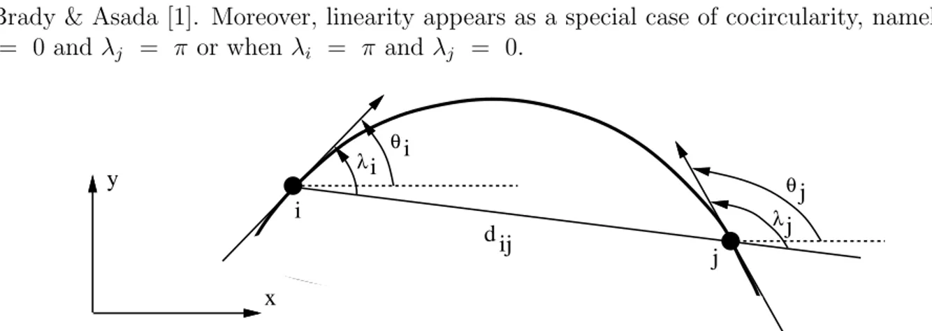
In this formula, λi is the angle made by one edgel with the line joining the two edgels. Notice that a circle is uniquely defined if the relative orientations of the two edgels verify the equation above. This equation is also a local symmetry condition consistent with the definition of local symmetry of Brady & Asada [1]. Moreover, linearity appears as a special case of cocircularity, namely when λi = 0 and λj = π or when λi = π and λj = 0.
λ λ θ θ x y d ij i j i j i j
Figure 3: The definition of cocircularity between two edgels i and j.
From this cocircularity constraint we may derive a weaker constraint which will measure the similarity between a two-edgel-configuration and a circular shape:
∆ij =| λi+ λj − π | .
∆ij will vary between 0 (a perfect circle) and π (no shape). Finally the cocircularity coefficient is constrained to vary between 1 for a circle and 0 for noise and is defined by the formula:
ccocirij = à 1 − ∆ 2 ij π2 ! exp à −∆ 2 ij k ! (4) The parameter k is chosen such that the cocircularity coefficient vanishes gently for non-circular interactions.
Smoothness. Consider an edgel and two nearby edgels. From Figure 4 it is clear that the cocircularity coefficient between edgels i and j is the same as the cocircularity coefficient between i and k. Indeed there are two circles, one passing through i and j and the other passing trhough i and k. One would like to give some preference to one of these configurations. If smooth curves (rather than rapidly turning curves) are prefered then the i − j interaction should be stronger than the i − k interaction.
With the same definition for λ as above we define a smoothness coefficient between two image edgels. This coefficient varies between 0 (a sharp corner) and 1 (a straight line):
csmoothij = Ã 1 − λi(π − λi) π2 ! Ã 1 − λj(π − λj) π2 ! (5)
i
j
k
Figure 4: In the absence of the smoothness constraint, the interaction between i and j is the same as the interaction between i and k (left). The smoothness constraint reduces the interaction in between parallel curves (right).
Obviously, for the example of Figure 4-left we obtain: csmoothij > csmoothik
Figure 4-right illustrates another advantage of using a coefficient that enforces smoothness. Indeed, the absence of the smoothness constraint, edgel interactions occur between parallel curves: an edgel equally interacts with its longitudinal neighbours and with its lateral neighbours. The smoothness constraint reduces the lateral interactions occuring between such parallel curves.
Proximity. The surrounding world is not constituted only by circular shapes. Cocircularity must therefore be a local property. That is, the class of shapes we are interested to detect at a given scale of resolution are shapes that can be approximated by a sequence of smoothly connected circular arcs and straight lines. The proximity constraint is best described by a coefficient that vanishes smoothly as the two edgels are farther away from each other:
cproxij = exp à − d 2 ij 2 σ2 d ! (6) where dij is the distance between the two edgels and σd is a fraction of the standard deviation of all these distances over the image. Hence, the edgel interaction will adjust itself to the image distribution of the edgel population.
Contrast. A classical approach to figure-ground discrimination is to compare the gradient value at an edgel against a threshold and to eliminate those edgels that fall under this threshold. An improvement to this simply-minded nonlinear filtering is to consider two thresholds such that edgel connectivity is better preserved [2]. Following the same idea, selection of shapes with high contrast can be enforced by multiplying the interaction coefficient with a term whose value depends on contrast:
ccontrastij = gigj g2
max
(7) gmax is the highest gradient value over the edgel population.
Finally the interaction coefficient between two edgels becomes: cij = ccocirij csmoothij c
prox
V
Mean field annealing (MFA)
The states reachable by the system described by eq. (1) correspond to the vertices of a N-dimensional hypercube. We are looking for the state which corresponds to the absolute minimum of the energy function. Typically, when N = 1000, the number of possible configurations is 2N ≈ 10301
. The problem of finding the absolute minimum is complex because of the large number of local minima of the energy function and hence this problem cannot be tackled with local minimization methods (unless a good initialization is available).
We already mentioned that the functional to be minimized has the same structure as the global energy of an interacting spin system. To find a near ground state of such a physical system we will use statistical methods. Two analysis are possible depending on the interaction of the system with its environment: either the system can exchange heat with its environment (case of the canonical analysis) or the system is isolated (case of the microcanonical analysis) [8]. We will consider here the canonical analysis.
This analysis makes the hypothesis that the physical system can exchange heat with its environ-ment. At the equilibrium, statistical thermodynamics shows that the free energy F is minimized. The free energy is given by: F = E − T S, where E is the internal energy (the energy associated with the optimization problem) and S is the entropy (which measures the internal disorder). Hence, there is a competition between E and S. At low temperatures and at equilibrium, F is minimal and T S is close to zero. Therefore, the internal energy E is minimized. However the minimum of E depends on how the temperature parameter decreases towards the absolute zero. It was shown that annealing is a very good way to decrease the temperature.
We are interested in physical systems for which the internal energy is given by eq. (1). The remarks above are expressed in the most fundamental result of statistical physics, the Boltzmann (or Gibbs) distribution:
P r(E(~σ) = Ei) =
exp (−Ei/(kT ))
Z(T ) (9)
which gives the probability of finding a system in a state i with the energy Ei, assuming that the system is at equilibrium with a large heat bath at temperature k T (k is the Boltzmann’s constant). Z(T ) is called the partition function and is a normalization factor:
Z(T ) =X n
exp (−En/(kT ))
This sum runs over all possible spin configurations. Using eq. (9) one can compute at a given tem-perature T the mean value over all possible configurations of some macroscopic physical parameter A: hAi =X n AnP r(E(~σ) = En) = P nAn exp (−En/(kT )) Z(T ) (10)
Unfortunately, the partition function Z(T ) is usually impossible to compute. Nevertheless, when the system is described by eq. (1) one can use eq. (10) which, with an additionnal hypothesis, is a basic equation for mean field approximation and for mean field annealing.
In order to introduce the mean field annealing algorithm, we first introduce the somehow more classical mean field approximation method which has been used to solve optimization problems
[13, 15, 9]: it is a simple analytic approximation of the behaviour of interacting spin systems in thermal equilibrium. We start by developing eq. (1) around σi:
E(σ1, σ2, . . . , σN) = Φiσi− 1 2 N X k=1,k6=i N X j=1,j6=i Jkjσkσj− N X k=1,k6=i δkσk
Φi is the total field which affects the spin σi:
Φi = − N X j=1 Jijσj+ δi
The mean field hΦii affecting σi is computed from the sum of the fields created on the spin σi by all the other spins ”frozen” in their mean states, and of the external field δi viewed by the spin σi. The mean state of a spin hσii is the mean value of the σi’s computed over all possible states that may occur at the thermal equilibrium. We obtain:
hΦii = − N X j=1 Jijhσji + δi (11)
We introduce now the following approximation [19]: The system composed of N interacting spins is viewed as the union of N systems each composed of a single spin. Such a single-spin system {σi} is subject to the mean field hΦii created by all the other single-spin systems. Let us study such a single spin system. It has two possible states: {−1} or {+1}. The probability for the system to be in one of these states is given by the Boltzmann distribution law, eq. (9):
P (Xi = σi0) ≈
exp (−hΦii σi0/T ) P (Xi = 1) + P (Xi = −1)
, σ0
i ∈ {−1, 1} (12)
Xi is the random variable associated with the value of the spin state. Notice that in the case of a single-spin system the partition function (the denominator of the expression above) has a very simple analytical expression. By combining eq. (10), (11), and (12), the mean state of σi can now be easily derived:
hσii ≈
(+1) exp (−hΦii/T ) + (−1) exp (hΦii/T ) exp (hΦii/T ) + exp (−hΦii/T )
(13) = tanh à PN j=1Jijhσji + δi T !
We consider now the whole set of single-spin systems. We therefore have N equations of the form: µi = tanh à PN j=1Jijµj + δi T ! (14) where µi = hσii. The problem of finding the mean state of interacting spin system at thermal equilibrium is now mapped into the problem of solving a system of N coupled non-linear equations, i.e., eq. (14). In the general case, an analytic solution is rather difficult to obtain. Instead, the
solution for the vector ~µ = [µ1, · · · , µN] may well be the stationary solution of the following system of N differential equations: τ dµi dt = tanh à PN j=1Jijµj + δi T ! − µi (15)
where τ is a time constant introduced for homogeneity. In the discrete case the temporal derivative term can be written as:
dµi dt ! tn = µ n+1 i − µni ∆t + o(∆t) (16) where µn
i is the value of µi at time tn. By substituting in eq. (15) and by choosing τ = ∆t, we obtain an iterative solution for the system of differential equations described by eq. (15):
∀ i ∈ {1, . . . , N }, µn+1i = tanh à PN j=1Jijµnj + δi T ! , n ≥ 1 (17) where µn
i is an estimation of hσii at time tn or at the n’th iteration. Starting with an initial solution ~µ0 = [µ0
1, · · · , µ 0
N] the convergence is reached at the n’th iter-ation such that ~µn = [µn
1, · · · , µnN] becomes stationary. The physicists would say that the thermal equilibrium has been nearly reached. When the vector ~δ is the null vector, one can start with a vector ~µ0 close to the obvious unstable solution [0, · · · , 0]. In practice, even when the vector ~δ in not null one starts with an initial configuration obtained by adding noise to [0, · · · , 0]. For instance the µ0
i’s are chosen randomly in the interval [−10−5, +10−5]. This initial state is plausible for an interacting spin system in a heat bath at high temperature. In fact the spin values (+1 or –1) are equally likely at high temperatures and hence, hσii = 0 for all spin i. During the iterative process, the µi’s converge to values in between −1 or +1.
Two convergence modes are possible:
• Synchronous mode. At each step of the iterative process all the µn
i’s are updated using the µn−1i ’s previously calculated.
• Asynchronous mode. At each step of the iterative process a spin µn
i is randomly selected and updated using the µn−1i ’s.
In practice, the asynchronous mode produces better results because the convergence process is less subject to oscillations frequently encountered in synchronous mode. In order to obtain a solution for the vector ~σ from the vector ~µ, one simply looks at the signs of the µn
i’s. A positive sign implies that the probability that the corresponding spin has a value of +1 is greater than 0.5:
(
if 1/2(1 + µn
i) > 0.5 then σi = +1
else σi = −1.
A practical difficulty with mean field approximation is the choice of the temperature T at which the iterative process must occur. To avoid such a choice one of us [10] and other authors [20] have proposed to combine the mean field approximation process with an annealing process giving rise to mean field annealing. Hence, rather than fixing the temperature, the temperature is decreased during the convergence process: thus the µi’s tend to +1 or −1 as the system converges.
V.A
Estimating the MFA parameters and good initial conditions
The MFA equations contain two parameters to be determined: the initial temperature Tinit and the decreasing factor of the temperature between two steps, decT . Moreover, the initial values of the µn
i’s should be independent of the image. The aim is to avoid a trial-and-error process: the algorithm should be a black box from a user’s perspective.
The initial temperature. The spin system onto which we have mapped the figure/ground discrimination problem typically has two phases; at high enough temperatures, according to the Boltzmann distribution, all the states reachable by the system are equally likely. As the temperature is lowered down, a phase transition occurs at T = Tc and as T → 0 the µivalues represent a specific decision made as to the solution to the problem. At convergence, these values verify:
1 N N X i=1 | µi |= 1 (18)
Untill now, we don’t know how to calculate the critical temperature of an interacting spin system when the external field is not null (i.e., when there is at least one δi that is not null). Practically, we use random asynchronous dynamics (which is the dynamics the most similar to the behaviour of a spin system). We start with a high enough initial temperature determined by the µi distribution: Each µi has to be around 0 at the beginning and during several iterations; otherwise, the initial temperature is increased.
Annealing schedule. As already mentioned, two different annealing schedules are possible: • Van den Bout & Miller [20] tried to estimate theoretically the critical temperature and then
they perform two sets of iterations: one iteration process at this critical temperature until a near equilibrium state is reached and another iteration process at a temperature value that is close to 0. However, the critical temperature is quite difficult to estimate and the behaviour of the spin system predicted by their analytical approximation is not in accordance with the computational experiments.
• Instead of estimating the critical temperature, we prefer the following schedule. Initially the temperature has a high value and as soon as every spin has been updated at least once, the temperature is decreased to a smaller value. Then the temperature continues to decrease at each step of the convergence process. This does not guarantee that a near equilibrium state is reached at each temperature value but when the temperature is small enough then the system is frozen in a good stable state. Consequently, the convergence time is reduced since at low temperatures the convergence to a stationary solution is accelerated. One of us has successfully used this strategy to solve hard, np-complete graph combinatorial problems [9], [10].
The initial values of the µi’s. When the vector ~δ (i.e., the external field) is the null vector, one can start with a vector ~µ0 close to the obvious unstable solution [0, · · · , 0]. In practice, when the vector ~δ is not null one starts with an initial configuration obtained by adding noise to [0, · · · , 0].
For instance the µ0
i’s are chosen randomly in the interval [−10−5, +10−5]. This initial state is plausible for a spin system in a heat bath at high temperature. In fact the spin values (+1 or –1) are equally likely at high temperatures and hence, hσii = 0 for all spin i (see equation (9)). During the iterative process, the µi’s converge to values in between −1 or +1.
The mean field annealing algorithm is outlined in the Appendix.
VI
Examples
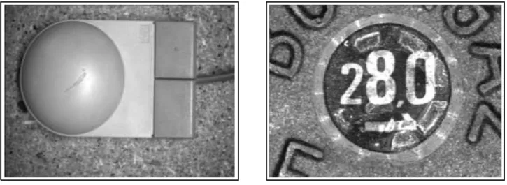
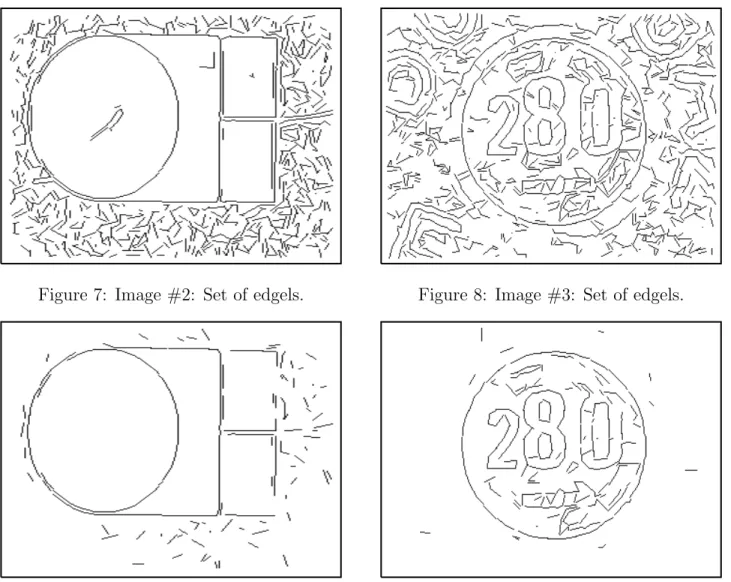
We tested these algorithms over a wide variety of images. Figure 5 and Figure 6 show two such im-ages. These images are preprocessed as follows. Edges are first extracted using the Canny/Deriche operator [4]. A small set of connected edges are grouped to form an edgel as follows: The tangent direction associated with such an edgel is computed by fitting a straight line in the least-square sense to the small set of connected edges. Then this small set of edges is replaced by an edgel, i.e., the fitted line. The position of the edgel is given by its midpoint, its direction is given by the direction of the line, and its contrast is given by the average contrast of the edges forming the edgel. Figure 7 and Figure 8 show the input data of our experiments.
Figure 5: Image #2. Figure 6: Image #3.
Figure 2 shows the result of applying mean field annealing to the synthetic data (image #1). Figure 9 and Figure 10 show the result of applying mean field annealing to the real images.
VII
Discussion
In this paper we attacked the problem of figure-ground discrimination with special emphasis on the problem of separating image data into curve and noise. We proposed a global approach using combinatorial optimization. We suggested a mathematical encoding of the problem which takes into account such image properties as cocircularity, smoothness, proximity, and contrast and this encoding fits the constraints of the statistical modelling of interacting spin systems. We described mean field annealing which is a deterministic approximation of simulated annealing and to which it compares favourably both in terms of robustness and efficiency. Indeed, equivalent sequential
Figure 7: Image #2: Set of edgels. Figure 8: Image #3: Set of edgels.
Figure 9: The result of applying MFA to im-age #2.
Figure 10: The result of applying MFA to im-age #3.
implementations of both algorithms (mean field annealing and simulated annealing) reveal that the former is of the order of 50 times faster than the latter [8]. Both simulated annealing and mean field annealing may be implemented on a fine-grained parallel machine – such an implementation is enforced by the analogy between the energy associated with an interacting spin system (such as ours) and the energy of a recursive neural network. With such an analogy, a neuron (or a processor) is associated with an edgel and each neuron communicates with all the other neurons. With such a parallel implementation and in synchronous mode (see section V) mean field annealing is N times faster than in asynchronous mode (where N is the number of edgels). Therefore the synchronous parallel implementation of mean field annealing is expected to be 50N times faster than the parallel implementation of simulated annealing.
In the future we plan to continue to try to improve our method in order to be able to eliminate all the noisy edgels, even those that are close to a shape and included in this shape by our current encoding. We also plan to try to solve other aspects of the image segmentation problem such as the feature grouping problem. We intend to extend the approach advocated in this paper to other
vision problems such as matching and reconstruction.
Appendix: The MFA algorithm
The following algorithm applies whenever the cost function associated with the combinatorial op-timization problem to be solved is of the form of eq. (1).
1. Fix the convergence mode (synchronous or asynchronous). Fix the initial temperature: T = Tinit = 100.
Fix the temperature decreasing factor between two consecutive iterations: decT = 0.9995. For all i, µ0
i is set to a random value in the interval [−10−5, 10−5]. Initialize an iteration counter: iter ← 0.
2. iter ← iter + 1.
Case of an asynchronous convergence mode: (a) ∀i, µold
i = µiter−1i .
(b) Scan at random the spins µi and iteratively update each spin µi see n in the scan (see equation (17)): i. Calculate µnewi = tanh à PN j=1Jijµoldj + δi T ! . ii. Update µi: µoldi ← µnewi .
(c) ∀i, µiter
i = µoldi .
Case of a synchronous convergence mode: for all spins µi, µiteri = tanh à PN j=1Jijµiter−1j + δi T ! . 3. If iter ≤ 5,
(a) decrease the temperature: T ← decT × T , (b) goto step 2.
4. Test if the algorithm has converged into a configuration different from the initial one: if
PN
i=1
Piter
l=iter−5 | µli |< 0, 99 × 6 × N , then the system has not converged: (a) decrease the temperature: T ← decT × T ,
(b) goto step 2.
5. The system has converged: assign the final values of the σi’s: ∀i, if µiteri > 0 then σi = 1 else σi = −1.
In practice we take Tinit = 10 and decT = 0.9995. At convergence the values of the µi’s are very close to either −1 or +1. In our experiments we have noticed that this is not the case with mean field approximation in which case the final values of the µi’s are less disriminative.
References
[1] M. Brady and H. Asada. Smoothed local symmetries and their implementation. International Journal of Robotics Research, 3(3):36–61, 1984.
[2] J. Canny. A Computational Approach to Edge Detection. IEEE Transactions on Pattern Analysis and Machine Intelligence, PAMI-8(6):679–698, November 1986.
[3] P. Carnevali, L. Coletti, and S. Patarnello. Image Processing by Simulated Annealing. IBM Journal of Research and Development, 29(6):569–579, November 1985.
[4] R. Deriche. Using Canny’s criteria to derive a recursively implemented optimal edge detector. International Journal of Computer Vision, 1(2):167–187, 1987.
[5] D. Geiger and F. Girosi. Parallel and deterministic algorithms from mrf’s: Surface reconstruc-tion. IEEE Transactions on Pattern Analysis and Machine Intelligence, 13(5):410–412, May 1991.
[6] D. Geiger and A. Yuille. A common framework for image segmentation. International Journal of Computer Vision, 6(3):227–243, 1991.
[7] D. Gutfinger and J. Sklansky. Robust classifiers by mixed adaptation. IEEE Trans. on Pattern Analysis and Machine Intelligence, PAMI-13(6):552–567, June 1991.
[8] L. H´erault and R. Horaud. Figure-ground discrimination: a combinatorial optimization ap-proach. IEEE Transactions on Pattern Analysis and Machine Intelligence, 15(9):899–914, September 1993.
[9] L. H´erault and J.J. Niez. Neural Networks and Graph K-Partitioning. Complex Systems, 3(6):531–576, December 1989.
[10] L. H´erault and J.J. Niez. Neural Networks and Combinatorial Optimisation: A Study of NP-Complete Graph Problems. In E. Gelembe, editor, Neural Networks: Advances and Ap-plications, pages 165–213. North Holland, 1991.
[11] M. Kass, A. Witkin, and D. Terzopoulos. Snakes: Active contour models. International Journal of Computer Vision, 1(4):321–331, January 1988.
[12] W. Kohler. Gestalt Psychology. Meridian, New-York, 1980.
[13] H. Orland. Mean field theory for optimization problems. Journal de Physique – Lettres, 46(17):L–763–L–770, September 1985.
[14] P. Parent and S.W. Zucker. Trace Inference, Curvature Consistency, and Curve Detection. IEEE Transactions on Pattern Analysis and Machine Intelligence, 11(8):823–839, August 1989. [15] C. Peterson. A new method for mapping optimization problems onto neural networks.
[16] C. Peterson. Track finding with neural networks. Nuclear Instruments and Methods in Physics Research, A279:537–545, 1989.
[17] T. J. Sejnowski and G. E. Hinton. Separating Figure from Ground with a Boltzmann Machine. In Michael Arbib and Allen Hanson, editors, Vision, Brain, and Cooperative Computation, pages 703–724. MIT Press, 1988.
[18] A. Shashua and S. Ullman. Structural Saliency: The Detection of Globally Salient Structures Using a Locally Connected Network. In Proc. IEEE International Conference on Computer Vision, pages 321–327, Tampa, Florida, USA, December 1988.
[19] H.E. Stanley. Introduction to Phases Transitions and Critical Phenomena. Oxford University Press, 1971.
[20] D.E. Van den Bout and T. K. Miller. Graph Partitioning Using Annealed Neural Networks. In Int. Joint Conf. on Neural Networks, pages 521–528, Washington D.C., June 1989.
[21] J. Zerubia and R. Chellappa. Mean field approximation using compound Gauss-Markov ran-dom field for edge detection and image restoration. In Proceedings of ICASSP, pages 2193– 2196, Alburquerque, New Mexico, USA, April 1990.