Bandwidth Scaling Behavior in Wireless Systems:
Theory, Experimentation, and Performance Analysis
by
Wesley M. Gifford
S.M., Massachusetts Institute of Technology (2004)
B.S., Rensselaer Polytechnic Institute (2001)
Submitted to the Department of Electrical Engineering and Computer Science
in partial fulfillment of the requirements for the degree of
Doctor of Philosophy in Electrical Engineering
at the
MASSACHUSETTS INSTITUTE OF TECHNOLOGY
September 2010
@ Massachusetts Institute of Technology 2010. All rights reserved.
.1 .A MASSACHUSETTS INSTiTUTE OF TECH4OLOGY
OCT J 5 2010
LIBRARIES
ARCHIVES
t, IA u th or ...
...
Department of Electrical Engir1ering and#'omputer Science
September 2, 2010
..C ertified by ... ...
...
Associate Professor
Thesis Supervisor
~1Accepted by...
...
Professor Terry P. Orlando
Chairman, Department Committee on Graduate Students
Bandwidth Scaling Behavior in Wireless Systems:
Theory, Experimentation, and Performance Analysis
by
Wesley M. Gifford
Submitted to the Department of Electrical Engineering and Computer Science on September 2, 2010, in partial fulfillment of the
requirements for the degree of
Doctor of Philosophy in Electrical Engineering
Abstract
The need for ubiquitous wireless services has prompted the exploration of using increasingly larger transmission bandwidths often in environments with harsh propagation conditions. However, present analyses do not capture the behavior of systems in these channels as the bandwidth changes. This thesis: describes the development of an automated mea-surement apparatus capable of characterizing wideband channels up to 16 GHz; formulates a framework for evaluating the performance of wireless systems in realistic propagation environments; and applies this framework to sets of channel realizations collected during a comprehensive measurement campaign. In particular, the symbol error probability of realistic wideband subset diversity (SSD) systems, as well as improved lower bounds on time-of-arrival (TOA) estimation are derived and evaluated using experimental data at a variety of bandwidths. These results provide insights into how the performance of wireless systems scales as a function of bandwidth.
Experimental data is used to quantify the behavior of channel resolvability as a function of bandwidth. The results show that there are significant differences in the amount of energy captured by a wideband SSD combiner under different propagation conditions. In particular, changes in the number of combined paths affect system performance more significantly in non-line-of-sight conditions than in line-of-sight conditions. Results also indicate that, for a fixed number of combined paths, lower bandwidths may provide better performance because a larger portion of the available energy is captured at those bandwidths.
The expressions for lower bounds on TOA estimation, developed based on the Ziv-Zakai bound (ZZB), are able to account for the a priori information about the TOA as well as statistical information regarding the multipath phenomena. The ZZB, evaluated using measured channel realizations, shows the presence of an ambiguity region for moderate signal-to-noise ratios (SNRs). It is shown that in a variety of propagation conditions, this ambiguity region diminishes as bandwidth increases. Results indicate that decreases in the root mean square error for TOA estimation were significant for bandwidths up to approximately 8 GHz for SNRs in this region.
Thesis Supervisor: Moe Z. Win Title: Associate Professor
Acknowledgments
The success of this thesis is due to the contributions of many people. I am grateful to my advisor, Professor Moe Win, whose mentoring, encouragement, and tireless energy have helped tremendously throughout the research process. I am also indebted to Professor Dennis Freeman and Professor Vivek Goyal for their helpful advice and feedback during my graduate program.
Most importantly, I would like to thank Stacey MacGrath for always being there when I need her. Without her support and encouragement, this dissertation would not have been possible. I also thank my parents and family for their unwavering support. I especially thank my father for his invaluable advice and assistance during the design and fabrication of the positioning subsystem.
I also thank my Italian colleagues, Professor Marco Chiani, Professor Davide Dardari, and Professor Andrea Conti. The success of this thesis is due to several fruitful collabora-tions with these colleagues, and I look forward to working with them in the future.
I thank my colleagues and friends in the Wireless Communications Group at LIDS for helpful discussions. I am especially grateful to Dr. Henk Wymeersch, Yuan Shen, Watcharapan Suwansantisuk, William Weiliang Li, Ulric Ferner, Stefano Marano, Dr. Pedro Pinto, and Megumi Ando.
This thesis was greatly facilitated by assistance along the way from: Joseph Gencorelli and Michael Ballou at Agilent Technologies, Douglas Pitts at Numatics Motion Control, and Riaan Booysen at Saab-Grintek.
I would also like to acknowledge support from the MIT Claude E. Shannon Endowment Fund, the John W. Jarve Fellowship, the Office of Naval Research Young Investigator Award N00014-03-1-0489, the Office of Naval Research Presidential Early Career Award for Scientists and Engineers (PECASE) N00014-09-1-0435, the National Science Foundation under Grants ANI-0335256, ECS-0636519, and ECCS-0901034, the Charles Stark Draper Laboratory, the Defense University Research Instrumentation Program under grant N00014-08-1-0826, and the MIT Institute for Soldier Nanotechnologies.
Contents
1 Introduction 25
1.1 Channel Characterization . . . . 26
1.2 Wideband Diversity... . . . . . . . . 27
1.3 Ranging Error Bounds . . . . 28
1.4 Contributions... . . . . . . . .. 29
1.5 Organization ... . . . . . . . . . 30
2 Measurement Apparatus 31 2.1 Positioning Subsystem... . . . . . . . .. 31
2.1.1 Configuration... . . . . . .. 32
2.1.2 Accuracy and Precision... . . . . . . .. 33
2.1.3 Sum m ary . . . . 35
2.2 Channel Measurement Subsystem... . . . . . . . . 35
2.2.1 Configuration... . . . . . . . . 36
2.2.2 Calibration... . . . . . . . . . . .. 38
2.2.3 Measurement Accuracy . . . . 43
2.2.4 Sum m ary . . . . 45
2.3 Computer Automation... . . . . . . . . . 45
2.3.1 Positioning and Channel Measurement Subsystems Control Software 46 2.3.2 Software and Data Organization... . . . . . . .. 47
2.3.3 Data Storage Format and Low-level Access Functions . . . . 47
2.3.4 Accessing Calibrated Data... . . . . . . .. 51
3 Measurement Campaign 55 3.1 Measurement Parameters . . . . 55
3.2 Measurement Locations... . . . . . . . . . 56
3.3 Measurement Grid... . . . . . 58
3.4 Data Processing... . . . . . . . . .. 59
3.4.1 Center Frequency-Bandwidth Domain... . . . . . . . . .. 59
3.4.2 Computation of the Time-Domain Representation... . . . .. 61
3.4.3 Channel Parameter Extraction Methodology... . . . . . . .. 64
3.5 Sample Channel Realizations... . . . . . . . .. 70
4 Wideband Subset Diversity Systems 73 4.1 System and Channel Model . . . . 75
4.1.1 Ideal Maximal-ratio Combining... . . . . . . . . 77
4.1.2 Ideal Selection and Combining ... . ... ... 78
4.1.3 Non-ideal Selection and Combining.... . . . . . . . 79
4.2 Analysis for Subset Diversity in Rayleigh Fading . . . . 81
4.2.1 Ideal Selection and Combining... . . . .. 81
4.2.2 Non-ideal Selection and Combining... . . . .. 83
4.2.3 Expressions for the Moment Generating Function of 1yj and 7N . - - 87
4.2.4 Error Probability Expressions... . . . . . .. 88
4.2.5 Special C ases . . . . 89
4.3 Analysis for Subset Diversity in Realistic Fading Channels . . . . 93
4.3.1 Ideal Selection and Combining... . . .. 94
4.3.2 Non-ideal Selection and Combining... . . . . .. 94
4.4 Numerical Results and Discussion... . . . . . .. 99
4.4.1 Comparison between Exact Analytical and Semi-analytical Results . 100 4.4.2 Number of Multipath Components... . . . . .. 101
4.4.3 SEP Performance in Realistic Channels.... . . . .. 105
4.5 Conclusion... . . . . . . . . . . . . 108
5 Improved Lower Bounds on Time-of-Arrival Estimation Error 113 5.1 Signal and Channel Models . . . . 116
5.1.1 Infinite Ensemble of Channel Realizations... . . .. 117
5.1.2 Finite Ensemble of Channel Realizations... . . . . . . . .. 119
5.3 Theoretical Limits in Ideal Propagation Conditions . . . . 121
5.3.1 The Cramer-Rao Bound in Ideal Conditions . . . . 122
5.3.2 The Ziv-Zakai Bound in Ideal Conditions . . . . 123
5.3.3 Numerical Examples Using UWB Pulses in AWGN . . . . 123
5.3.4 Extending the Bounds to the Multipath Case . . . . 125
5.4 Receiver with Perfect Knowledge of the CPR . . . . 126
5.4.1 Cramer-Rao Bound... . . . . . . . . . 126
5.4.2 Ziv-Zakai Bound . . . . 128
5.5 Receiver with Statistical Knowledge of the CPR . . . . 131
5.5.1 Cramer-Rao Bound... . . . . . . . . . . . . . 131
5.5.2 Ziv-Zakai Bound.. . . . . . . . 133
5.6 Numerical Results... . . . .. 140
5.6.1 Infinite Ensemble of Channel Realizations . . . . 140
5.6.2 Finite Ensemble of Channel Realizations. . . . . . . . 145
5.7 Conclusion... . . . . . . . .. 148
6 Conclusion 151 6.1 W ideband Diversity Systems . . . . 151
6.2 TOA Estimation Error Bounds... . . . . . . . . 152
6.3 Future W ork .. . . . . . . . 153
A Distribution of the Decision Variable for the Case of NSNC in Rayleigh
Fading 155
B Cramer Rao Bound Using the Averaging Bounding Approach 159
C Derivation of the Statistics of q(1) and q(2) 161
List of Figures
2-1 The channel measurement apparatus: (a) the positioning subsystem and measurement hardware, (b) the transmit antenna mounted at the top of the tripod, along with the amplifier and coupler located near the base of the trip o d . . . . . 32
2-2 Setup of the measurement system... . . . . . . . . . 35
2-3 Azimuth and elevation patterns for the wideband antennas used by the chan-nel measurement apparatus. Note that the azimuth pattern is extremely uniform and the elevation beamwidth is very broad at a particular frequency. 38 2-4 The manufacturer provided gain data of the antennas, averaged over azimuth
angle, is within i1 dBi of the average over frequency. . . . . 39
2-5 The measurement layout for the antenna calibration procedure. Circles indi-cate the position of the transmit antenna and crosses indiindi-cate the position of the receive antenna along arcs with a radius of 1 m. The large black square indicates the positioning area of the channel characterization apparatus. . . 41
2-6 Magnitude and phase of the average response of the pair of antennas at a distance of 1 m . . . . 42 2-7 Passband impulse response of the pair of antennas, resulting from the
cali-bration procedure described in Sec. 2.2.2. . . . . 42
2-8 Magnitude and phase of the reflection coefficient (S1 1) of the antennas used
in the channel measurement apparatus. Note that the magnitude is approx-imately less than -10 dB and the phase is nearly linear. . . . . 43
3-1 Measurements were made on the 6th floor of the Dreyfoos tower of the Ray and Maria Stata Center. The blue squares indicate the locations where chan-nel responses were captured (in each location the black triangle depicts the origin of the measurement grid). In all, measurements at 21 locations were
captured. ... ... ... ... 57
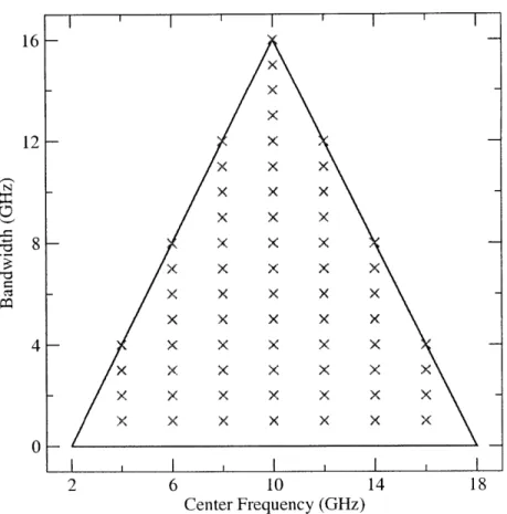
3-2 (a) The overall measurement grid: blue crosses make up the outermost grid of uncorrelated points, magenta circles make up an inner denser correlated grid, and green pluses make up small dense grids in the corners. (b) A detailed view of the lower left corner, showing the 49 points that make up this portion of the grid . . . . . 60 3-3 The set of possible center frequency and bandwidth pairs. The crosses
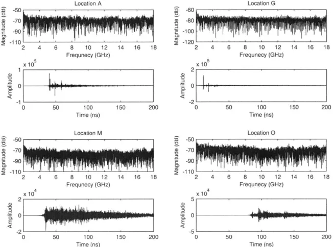
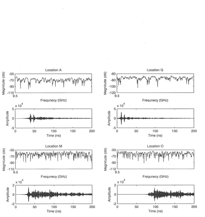
indi-cate the discrete pairs that were considered (Ss). . . . . 61 3-4 The magnitude of the frequency responses and the passband time-domain
responses are shown for four sample realizations, normalized to have unit energy, at 16 GHz bandwidth with
fc
= 10 GHz. . . . . 71 3-5 The magnitude of the frequency responses and the passband time-domainresponses are shown for four sample realizations, normalized to have unit energy, at 1 GHz bandwidth with
fc
= 10 GHz. . . . . 72 4-1 The basic structure of a RSSD receiver. . . . . 81 4-2 A portion of the received signal constellation, and its associated decisionregions. . . . . 84 4-3 A portion of the received signal constellation, and its associated decision
regions for the non-ideal case. In this example, consider the transmission of the symbol s7. The conditional symbol error probability (SEP) is computed with respect to the point &s7 which can either fall inside the decision region for s7 (a), or outside the decision region for S7 (b). . . . . 97
4-4 Exact analytical and semi-analytical SEP results for independent, identically distributed (ID) Rayleigh fading with Nd = 64 paths, Ld = 4, 16, 32 and Np E = 2, 16. Semi-analytical results agree with exact analytical expressions. 100
4-5 Number of paths output by the search-subtract-readjust algorithm for four representative locations in the measurement environment at a fixed band-width of 1 GHz. There are only minor variations in the number of paths as
a function of center frequency. . . . . 101
4-6 Number of paths output by the search-subtract-readjust algorithm for four representative locations in the measurement environment at a fixed center frequency 10 GHz. The curves display a saturation phenomena as bandwidth is increased, and the effect is more pronounced in dispersive environments. . 102 4-7 Number of paths output by the search-subtract-readjust algorithm for
loca-tion A as a funcloca-tion of bandwidth for five different center frequencies. The curves display a similar saturation phenomena as bandwidth is increased, regardless of center-frequency. . . . . . 104
4-8 Path energy capture for measurement locations A, G, M, and 0. . . . . 106
4-9 SEP at location A for 1 GHz bandwidth, Np E= 2, 16 and Ld = 4, 16, 32. 107
4-10 SEP at location G for 1 GHz bandwidth, NpE = 2, 16 and Ld= 4, 16, 32. 108
4-11 SEP at location M for 1 GHz bandwidth, Np E= 2, 16 and Ld = 4, 16, 32. 109
4-12 SEP at location 0 for 1 GHz bandwidth, Np E= 2, 16 and Ld= 4, 16, 32. 110
4-13 SEP at locations A, G, M, and 0. Curves are shown for Np
E=
2 at 1 GHz and 16 GHz bandwidths with Ld= 2, 4, 16, 32. . . . .111 4-14 SEP as a function of bandwidth at Ftot = 15 dB at locations A, G, M, and0. Curves are shown for Np E = 2 (solid lines) and NpE = 16 (dashed lines) with Ld = 2, 4, 8, 16, 32. . . . . 112 5-1 Cramer-Rao bound (CRB) and Ziv-Zakai bound (ZZB) on the root mean
square error (RMSE) as a function of signal-to-noise ratio (SNR) in an ad-ditive white Gaussian noise (AWGN) channel with Ta = 100 ns and
fc
= 4GHz. Bandpass 2nd-order Gaussian monocycle pulses with o- = 0.79 ns and o = 2.54 ns, as well as bandpass root raised cosine (RRC) pulses withv = 0.6, rp = 1ns and Tp = 3.2 ns, respectively, are considered. Coherent and noncoherent estimators are shown... . . . . . . . . . 125
5-3 ZZB and CRB on the RMSE, using the averaging bounding approach, as a function of SNR for the Rayleigh fading channel model with L = 1, 2, 4, 8. The CRB is also shown for coherent and noncoherent detection in AWGN. . 141 5-4 ZZB and CRB, using the averaging bounding approach, on the RMSE as
a function of SNR for the Rice/Rayleigh channel model with L = 1 and K = 0, 4, 8, 12 dB. In this channel model the first path is Ricean distributed and the remaining paths are Rayleigh distributed. The CRB is also shown for coherent and noncoherent detection in AWGN. . . . . 142 5-5 ZZB and CRB, using the averaging bounding approach, on the RMSE as a
function of SNR for the Rice/Rayleigh channel model. Rice factor K = 10 dB is considered with L = 1, 2, 4, 8. The CRB is also shown for coherent and noncoherent detection in AWGN... . . . . . . . . . . ... 143 5-6 ZZB and CRB, using the averaging bounding approach, on the RMSE as a
function of SNR for different power delay profiles and channel models with L = 8. The CRB is also shown for coherent and noncoherent detection in AWGN. The channel models considered are: 1) uniform power delay profile (PDP) with Rayleigh distributed paths, 2) uniform PDP with the first path Rice distributed (K = 10 dB) and the remaining paths Rayleigh distributed, and 3) exponential PDP with Rice distributed paths according to (5.86). . . . . 144 5-7 ZZB on the RMSE calculated using the various approximation methods
de-scribed in 5.5.2 for the Rayleigh fading channel model with L = 4 paths. The Schwartz-Yeh method and the maximum-mean method have nearly identical
performance... . . . . . ... 145
5-8 ZZB on the RMSE calculated using the various approximation methods de-scribed in 5.5.2 for the Rice/Ricean channel model with L = 4 paths and K = 10 dB. The Schwartz-Yeh method and the maximum-mean method have nearly identical performance. We can see that the maximum-mean method provides a good approximation when there is a specular component. . . . . 146 5-9 ZZB on the RMSE as a function of SNR for locations A, G, 0, and M with
Ta = 100 ns and
fc
= 10 GHz. Bandpass RRC pulses with v = 0.6 at various bandwidths are considered... . . . . . . . ... 1475-10 ZZB on the RMSE as a function of bandwidth for locations A, G, 0, and M with Ta = 100ns and
fc
10 GHz. Bandpass RRC pulses with v = 0.6 atList of Tables
2.1 Components used in the positioning subsystem . . . . 33 2.2 Amplifier specifications. The Herotek amplifier was used initially, but was
later replaced by the Lucix amplifier. . . . . 36 2.3 Coupler specifications... . . . . . . . . 36 2.4 Cable specifications... . . . . . . . . . . . . . 36 2.5 Description of the contents of the results parameter (.mat) file used to store
parameters of the measurements.... . . . . . . ... 48 2.6 Description of the pt-param structure that is used to store positioning
sub-system param eters . . . . 48 2.7 Description of the instr.param structure that is used to store channel
mea-surement subsystem parameters... . . . . . . . . 49 2.8 Specifications for the binary record format used when storing the
measure-ment data in the results dataset (.bin) file . . . . 50 2.9 Description of the instr-param structure that is used to store channel
mea-surement subsystem parameters... . . . . ... 53
3.1 Details of the measurement locations. Coordinates are given with reference to the origin shown in Fig. 3-1, the orientation angle is measured in a counter-clockwise direction from the x-axis of the origin to x-axis of the positioning grid, and the reported distances are with respect to the location of the trans-mitter (2.584, 14.653)... . . . ... 58
4.1 Parameters for MQAM signaling constellations . . . . 90 4.2 Expressions for PeNSNC(F) under specific selection policies and modulation
List of Notation
Matrix transposeConjugate transpose Matrix inverse
The Kronecker product of the matrices
a11B A o B=i amiB A and B. If A is an m x n matrix ... amnB Complex conjugate Trace of a matrix Determinant of a matrix Expectation Variance Covariance Probability Inner product Real part Imaginary part
The set consisting of elements ai, a2,..., aN
(.)T (-)t AoB tr{-} det{-} E{-} V{-} Cov{} Pr{-}
K0
N 9i{c} d3{c}{ai}Yi
List of Acronyms
AWGN additive white Gaussian noise
SNR signal-to-noise ratio
UWB ultrawide bandwidth
VNA vector network analyzer
IF intermediate frequency
IDFT inverse discrete Fourier transform FFT fast Fourier transform
IFT inverse Fourier transform
FT Fourier transform
SS spread spectrum
WSSUS wide-sense stationary uncorrelated scattering
RSSD Rake subset diversity
SP
single path
ARake all Rake
SRake selective Rake
MFEP matched front-end processor
BEP bit error probability SEP symbol error probability
SSD subset diversity
MRC maximal-ratio combining
H-S/MRC hybrid selection/maximal-ratio combining
RV random variable
IID independent, identically distributed
PDF probability density function MGF moment generating function
CF characteristic function
MSE mean square error
MMSE minimum mean square error
RMSE root mean square error LSE least squares estimate
LLSE linear least squares estimate
ML maximum likelihood
LRT likelihood ratio test
LR likelihood ratio LLR log-likelihood ratio CRB Cramer-Rao bound ZZB Ziv-Zakai bound ZZBT Ziv-Zakai Bellini-Tartara LOS line-of-sight
NLOS non-line-of-sight
GPS Global Positioning System
TOA time-of-arrival
UWB ultrawide bandwidth
TH time-hopping
PPM pulse position modulation
PDP power delay profile
WWB Weiss-Weinstein bound
CPR channel pulse response LRT likelihood ratio test RRC root raised cosine PDP power delay profile
Chapter 1
Introduction
The emergence of ubiquitous wireless services has prompted the exploration of using increas-ingly large bandwidth transmission, often in challenging environments and over bandwidths that are already in use for legacy systems. Current demands in quality and reliability of wireless connections suggest that ever-higher bandwidths in various frequency bands be made available in an unlicensed manner for unrestricted wireless access. Along this line, ultrawide bandwidth (UWB) spread spectrum systems have received considerable attention from the scientific, commercial and military sectors [1-15].
The use of extremely large transmission bandwidth results in desirable capabilities, in-cluding: 1) accurate positioning and ranging, and lack of significant multipath fading due to fine delay resolution; 2) simple implementation for multiple access communications; and 3) superior obstacle penetration due to low frequency components [3-7]. Interest in UWB systems has intensified owing to a ruling by the United States Federal Communications Commission (FCC) concerning UWB emission masks.1 This ruling is flexible enough to allow various implementations that satisfy the emission mask condition [16], enable UWB to coexist with traditional and protected radio services, and permit the use of UWB trans-mission without allocated spectrum.
Among other advantages, UWB systems inherently provide covert communication due to low power operation in an extremely large transmission bandwidth combined with spread spectrum techniques. UWB systems possess low probability of detection and interception (LPD/LPI) as well as anti-jam capabilities. By virtue of their robustness against fading
and superior obstacle penetration, UWB systems allow reliable communication in extremely challenging environments, where there are obstacles and dense multipath. Examples include dense urban areas, confined areas, within buildings, onboard vehicles, and in shipyards. It is known that current communication systems used by the military and emergency services do not perform well, or may fail altogether, under such conditions. UWB networks promise reliable, low-power and high-speed services for time-critical information to be relayed to its destination even in such challenging environments. Consequently, UWB systems are under consideration for many applications, including high-speed short-range WiFi, emergency services, military communications networks, sensor networks, and homeland defense systems
[10-15].
1.1
Channel Characterization
Characterization of wideband channels requires precise measurements over a very large bandwidth. Typically this is done using two methods: 1) time-domain based channel sound-ing ussound-ing very short duration pulses and a digital samplsound-ing oscilloscope, and 2) frequency-domain based channel measurement using a vector network analyzer (VNA). The first method uses a pulse generator to generate short pulses and a digital sampling oscilloscope to sample the channel response. Usually a series of pulses, modulated by a pseudo-random sequence, are transmitted to improve the SNR and produce more reliable measurements. These specialized channel sounders can be prohibitively expensive and are generally not widely available. Channel sounders also have limited dynamic range because they operate over the entire bandwidth of interest and hence are subject to the broadband noise floor.
Using the time-domain based method, extensive UWB propagation measurement cam-paigns have previously been performed in a modern laboratory/office building with the goal of characterizing the channel [3-7]. For these campaigns, a nanosecond-wide pulse was transmitted periodically with a repetition rate of 2 x 10⁶ pulses per second.
The research described in this thesis made use of the second method to measure channel responses in the frequency domain over the 2-18 GHz range. VNAs use a swept sine wave stimulus and therefore have better dynamic range, because the measurement is only made over the intermediate frequency (IF) bandwidth; a much smaller bandwidth. VNAs also come equipped with built in error correction capabilities which can correct for errors induced
by cables and impedance mismatches. Using this method it is easier to characterize the propagation channel over various bandwidths, since the measured responses can simply be filtered. The time-domain response can easily be computed using the inverse Fourier transform of the measured frequency response. A recent measurement campaign using a VNA to measure the 3-10 GHz frequency range is available in [17].
1.2
Wideband Diversity
Multipath diversity using spread spectrum (SS) signaling [18-25] has played an increas-ingly important role in current and future wireless systems. Wide transmission bandwidths available in SS systems allow receivers to resolve closely spaced multipath components. The detection of signals in multipath environments is typically done using a Rake receiver, where the components of a received signal (arriving at different delays) are combined to provide diversity. Discussions on classical Rake architectures can be found in [18-21]. One version of the Rake receiver consists of multiple correlators (fingers); each correlator detecting the signal from one of the multipath components created by the channel. The outputs of the Rake fingers are then combined to achieve the benefits of multipath diversity.
The complexity and performance issues associated with combining all the available mul-tipath components have motivated studies of receivers that process only a subset of the available resolved multipath components. Such Rake subset diversity (RSSD) receivers are a way to reduce resource use in receiver designs while maintaining the benefits of full diversity order [26-29]
Practical RSSD receivers must estimate the channel gain affecting each multipath com-ponent, and thereby incur a performance loss [30-35]. This is in contrast to many previous studies of RSSD which assumed that perfect channel knowledge is available at the receiver. In the case of practical RSSD, the estimation plays a dual role; it affects both the selec-tion process as well as the combining mechanism. Indeed, in an RSSD receiver the subset of multipath components chosen is based on the receiver's knowledge of the channel, i.e., the estimated channel gains. Therefore, there is the possibility that the receiver makes an erroneous selection.
1.3
Ranging Error Bounds
One of the primary advantages of ultra wideband communication is the fine delay resolu-tion that results from wide transmission bandwidth. For this reason, wideband systems are receiving increasing attention for use in ranging and localization systems. One way these systems operate is by time-of-arrival (TOA) estimation, where the first path of the received signal is detected to form an estimate of the distance from transmitter to receiver. However, when operating in dense multipath environments these systems are affected by errors induced by phenomena such as direct path blockage and direct path excess delay.
In some areas of the environment the direct path to a transmitter may be completely obstructed, so that the only received signals are from reflections, resulting in measured ranges larger than the true distances. Direct path excess delay occurs when the partially obstructed direct path propagates through different materials, such as walls. When such a partially obstructed direct path signal is observed as the first arrival, the propagation time depends not only upon the traveled distance, but also upon the materials it encountered. Because the propagation of electromagnetic signals is slower in some materials than in the air, the signal arrives with excess delay, again yielding a range estimate larger than the true one. It is important to note that the effect of direct path blockage and direct path excess delay is the same: they both add a positive bias to the true range, so that the measured range is larger than the true value. This positive error has been identified as a limiting factor in UWB ranging performance and it must be taken into account [36,37].
While the performance of a specific TOA estimation algorithm can be evaluated, esti-mation error bounds play a fundamental role since they can serve as useful performance benchmarks for the design of TOA estimators. The CRB has been widely used as a perfor-mance benchmark for assessing estimation error. However, it is well known that the CRB can be very loose at low and moderate SNR. Other bounds, such as the ZZB, can be applied to a wider range of SNRs and account for both ambiguity effects and a priori information of the parameter to be estimated. It is expected that as the bandwidth increases, the bound on the TOA estimation error will decrease, because larger bandwidth yields finer delay res-olution. However, there may be a point where the improvement diminishes. Understanding the point at which this occurs is valuable to system engineers.
1.4
Contributions
This thesis first describes a channel measurement apparatus that was designed and built to accurately characterize wideband propagation channels over a frequency range of 2-18 GHz. This frequency range represents more than double the bandwidth of conventional UWB systems. The apparatus contains an automated positioning subsystem, responsible for positioning the receive antenna, to enable accurate and rapid collection of channel responses. The extremely wide measurement bandwidth allows for the investigation of the effects of bandwidth at ranges beyond those currently available in the literature. The data collected using this apparatus is used in the subsequent chapters to make conclusions about the effects of bandwidth in realistic propagation environments.
This thesis characterizes the SEP performance of wideband subset diversity (SSD) sys-tems operating in multipath channels. These syssys-tems operate by selecting and combining a subset of the resolvable multipath components. Analytical expressions are developed for the case of non-ideal channel estimation, where the selection and combining process occur in the presence of channel estimation error. Two channel models are considered. The first considers a wide-sense stationary uncorrelated scattering (WSSUS) channel with a constant PDP. The second considers the case where only a set of channel realizations is available. In this case, the expressions are semi-analytical in nature-they are based on Monte-Carlo averaging of exact conditional SEP expressions. The analysis is valid for arbitrary two-dimensional signaling constellations and the expressions give insight into the performance losses of non-ideal SSD when compared to ideal SSD. Due to estimation error, these losses occur in branch combining as well as in branch selection. The SEP performance as a func-tion of bandwidth is investigated under different propagafunc-tion condifunc-tions. Results indicate that increased bandwidth yields more multipath components, and thereby increases the diversity present in the channel. However, operation at 1 GHz bandwidth provides better performance in terms of SEP because there is significantly more energy present in each path.
This thesis also investigates lower bounds on TOA estimation error for wideband and UWB ranging systems operating in realistic multipath environments. The thesis specifically considers developing bounds on TOA estimation for two cases: 1) when a statistical model of the multipath phenomena is available and 2) when only a finite set of channel
realiza-tions are available. In particular, analytical expressions for the CRB and ZZB on TOA estimation error for dense multipath channels are provided and discussed under different operating conditions. It is shown that for practical values of the SNR the classical CRB does not properly account for multipath effects and hence one needs to resort to improved bounds, such as those based on the ZZB. Using these bounds it is also shown how a priori knowledge about the multipath characteristics can improve TOA estimation performance. Furthermore, these bounds serve as useful performance benchmarks for the design of TOA estimators.
1.5
Organization
This thesis is organized as follows. Chap. 2 describes the channel measurement apparatus, including the positioning and measurement subsystems, as well as the software developed to control them. Chap. 3 gives specific details about the measurement campaign that was performed on the MIT campus, how the captured waveforms were processed, and describes the procedure for extracting the gains and delays from individual channel responses. Chap. 4 develops a framework for investigating the performance of non-ideal wideband diversity systems, both for theoretical models and measured channel responses. Chap. 5 develops a framework for the evaluation of the CRB and ZZB on the TOA estimation error of wideband signals affected by multipath propagation.
Chapter 2
Measurement Apparatus
This chapter describes a channel measurement apparatus that was custom designed and fabricated to precisely measure extremely wideband wireless channels. The measurement
apparatus consists of two major components: 1) the positioning subsystem, and 2) the wireless channel measurement subsystem. Care was taken in designing both subsystems to maximize the fidelity of the measurement data, while maintaining the flexibility of the overall apparatus. The complete channel measurement apparatus, including the transmit
antenna, is shown in Fig. 2-1. The next sections describe the positioning and channel mea-surement subsystems, as well as the associated calibration procedures. Finally, a detailed discussion of the software developed to control the measurement apparatus is presented.
2.1
Positioning Subsystem
In order to understand and predict the performance of systems operating in realistic en-vironments, it is first necessary to understand the statistical nature of the communication channel. To develop statistical models for the communication channel, one must capture numerous channel realizations. Typically, each of these channel realizations is collected by fixing the transmit and receive antenna, transmitting a known signal, and capturing the response. Then, the position of the receive antenna is moved to the next point and the process continues. Once all the measurements have been captured over a small-scale grid, additional measurements are then made by moving the small-scale grid to a new loca-tion. Since manual positioning of the transmit and receive antenna to collect this data can be time consuming, tedious, and error prone, the measurement apparatus incorporates an
(a) (b)
Figure 2-1: The channel measurement apparatus: (a) the positioning subsystem and mea-surement hardware, (b) the transmit antenna mounted at the top of the tripod, along with the amplifier and coupler located near the base of the tripod.
automated positioning subsystem to position the receive antenna.
2.1.1 Configuration
The positioning subsystem consists of a mobile cart, three linear motion units, and the necessary motors and motor controllers. The mobile cart was constructed primarily of non-metallic materials, including wood, plastic, fiberglass, and other composites to minimize any effects on the propagation environment. It measures 1.73 m x 1.22 m, and was designed to support the linear motion units, as well as the measurement hardware, while still allowing mobility. The mobile cart was also designed with enough space below the linear motion units to store the measurement and control hardware, creating a self-contained measurement apparatus.
The linear motion units, typically used in factory automation applications, offer speed and precision in positioning. Each unit consists of a track and a saddle which rides in the track. The saddle is connected to a timing belt which runs over two timing pulleys located at the ends of the track. One of the timing pulleys, the drive pulley, is rotated by a stepper motor. A Cartesian positioning grid is formed using these three units. Two units, parallel to each other and linked by a common drive shaft, form the y-axis. The third unit, perpendicular to the other units, is mounted on top of the saddles of the lower units to form the x-axis. The receive antenna is mounted on a small platform located on the
Name Mfr. Name, Model (Alt. Mfr. Name, Model) Linear motion units Numatics, BDU 75 (Warner, Rapidtrak M75) Motor controllers Numatics, NSDP6C (Superior Electric,
SS2000D6i)
Stepper motors Numatics, FLM9310 (Superior Electric, KM093)
X-axis gearbox GAM, EPL-N34-003G Y-axis gearbox CAM, HPS-TB-075-003G X-axis coupler Lovejoy, L-070
Y-axis couplers GAM/Jakob, EKZ 20/304
Table 2.1: Components used in the positioning subsystem
saddle of the top axis. Each linear motion unit is about 1.8 m long and is capable of 1.2 m of travel. The distance moved for every rotation of the drive pulley, referred to as the drive ratio, is 12.98 cm/rev. The two axes allow positioning the receive antenna anywhere in a 1.2 m x 1.2 m grid. The positioning subsystem can be seen in Fig. 2-1 and details about the components can be found in Table 2.1.
Movement of each axis of the positioning grid is accomplished by a stepper motor mounted to a low-backlash, high precision, 3:1 gear-reducer. The stepper motors have 200 full steps per revolution (1.8' per step), but are operated in micro-stepping mode (with one microstep equal to 1/64-th of a full step). A separate stepper motor drive controller is responsible for controlling each the stepper motors. The motor controllers have internal microprocessors which control the motion profile of each axis and enable the user to issue configuration and control commands over a serial interface.
Each axis of the positioning grid has three position sensors. Two of these sensors are used as end of travel limit sensors. These protect the linear motion units from damage if the saddle attempts to travel past the end of the unit. The third sensor, or home sensor, is used to determine the origin of the axis. The motor controller software includes commands that use the end of travel limit sensors and the home sensor to calibrate the axis. These sensors are also used to check the accuracy of the positioning subsystem.
2.1.2
Accuracy and Precision
Accuracy refers to the degree to which a measurement is close to the true value. Precision, or repeatability, is the degree to which measurements show the same results. There are several factors affecting the overall accuracy and precision of the positioning subsystem. In
the context of the positioning subsystem, accuracy refers to how closely the desired position matches the actual position. Precision refers to how close repeated movements to the same location are to one another. An ideal positioning system will have both high accuracy and precision. Below we discuss the individual components of the positioning subsystem and their effect on the overall accuracy and precision.
The overall accuracy and precision of the positioning subsystem is ±1 mm and 0.42 mm, respectively. This level of accuracy and precision is acceptable, since, during experiments, the mobile cart must be moved to locations where measurements will be taken. The coordi-nates of this location are recorded, to be able to understand propagation conditions and to calculate the true distance between the transmit and receive antennas. It is extraordinarily difficult to position the cart and measure its location with greater accuracy than that of the positioning subsystem.
The positioning subsystem has high resolution, since the motor controllers are config-ured to operate in micro-stepping mode with 1/64-th step resolution. This gives 12,800 mi-crosteps per revolution of the stepper motors or a final positioning resolution of < 0.0034 mm for each axis. The accuracy and precision of the positioning subsystem is dominated by the linear motion units, where the main contributing factor is the interaction between the tim-ing belt and timtim-ing pulleys. The specified positiontim-ing accuracy of the linear motion units is ±0.8333 mm/m and the repeatability is ±0.3 mm. This contributes ±1.2 x 0.8333 = 1.00 mm and +0.3 mm to the accuracy and repeatability, respectively.
Other components in the system also contribute to the overall accuracy and precision. However, their effects are much less significant. The stepper motors themselves are accurate to within ±2% of a full step, non-cumulative. These errors do not accumulate as the number of steps increases because of the way stepper motors are designed. Thus, the positioning accuracy of the stepper motors is ±2%.129.79/(3-200) = ±0.0043 mm-significantly smaller than the accuracy of the linear motion units. The gearboxes also contribute to the accuracy and precision. Backlash is a term that refers to the clearance between mating components, in our case the gears in the gear reducers, in a mechanical device. It can be thought of as the amount of lost motion when movement is reversed and contact between the gears is re-established. This affects the precision of the positioning system, but again, the effects are less significant than the precision of the linear motion units. The gear reducers have an output backlash of <10 arcmin and <6 arcmin for the x-axis and y-axis, respectively. This
Tx Antenna Rx Antenna
((X
))
~25m
Figure 2-2: Setup of the measurement system
creates an additional positioning uncertainty of t0.060 mm and ±0.036 mm, respectively.
2.1.3
Summary
The positioning subsystem enables extremely flexible positioning of the receive antenna. Grid layouts which would be very difficult to achieve with manual positioning, are now pos-sible with the positioning subsystem. Furthermore, moving from one grid point to the next takes less than a few seconds compared to several minutes for manual positioning. Also, the accuracy achieved through automated positioning is far better than one can achieve with manual positioning. This allows for accurate and extremely rapid data collection. The con-venience and accuracy of automated positioning comes with the cost of additional hardware and the presence of this hardware during the measurements. Ideally, channel measurements are taken to capture the propagation environment only. However, in a practical setting, these measurements will capture the effect of the environment and all the objects in it, including the measurement hardware. No matter the setup, it is impossible to remove all the effects of the measurement hardware.
2.2
Channel Measurement Subsystem
A VNA makes up the core of the channel measurement subsystem. VNAs are capable of ac-curately measuring the incident, reflected, and transmitted signals associated with a device under test. VNAs operate as a stimulus-response system: a known signal is transmitted and the resulting signals are measured. The channel measurement subsystem uses an
Agi-Location Mfr. Name, Output Power Gain (dB) Noise Figure
Model
(dBm)
(dB)
Transmit path Lucix, 20 24 3.5
S001200L2405
Receive path Herotek, 8 18 2.8
AF0120183A
Receive path Lucix, 20 24 3.5
S001200L2405
Table 2.2: Amplifier specifications. The replaced by the Lucix amplifier.
Herotek amplifier was used initially, but was later
Mfr. Name, Model Frequency Coupling Directivity Insertion
Range Factor Loss
Krytar, 152013 0.5-20 GHz 13±1.0 dB >15 dB <1.4 dB
Table 2.3: Coupler specifications
lent E8362B VNA to measure the frequency response of wireless channels over a frequency range of 2-18 GHz. The measurement setup is shown in Fig. 2-2. The subsequent sections describe the configuration of the measurement system in detail, the sources of error in the system, and the steps taken to mitigate them.
2.2.1 Configuration
The channel measurement subsystem makes use of two vertically polarized, omni-directional wideband antennas that radiate over a frequency range of 2-18 GHz. The azimuth and elevation antenna patterns are shown in Fig. 2-3. The antenna patterns indicate that the antennas have a very flat gain across their azimuth and a broad elevation beamwidth. The
Location Mfr. Name, Model Lengths (in) Loss (dB/m) @
18 GHz
Tx-VNA connection Florida RF, LabFlex 25 0.656
290AW
Rx-VNA connection Huber-Suhner, Sucofiex 5 1.6
104PE
Tx interconnections Megaphase, 0.10, 0.13, 0.33 2.17
Conformable Jumper
CC141
Rx interconnections Megaphase, SuperFlex 0.30, 0.46, 0.76 1.55 SF26
gain, averaged over azimuth angle, as a function of frequency is shown in Fig. 2-4. The figure indicates that the average gain, relative to an isotropic radiator, of the transmit and receive antennas are closely matched and is nearly uniform over frequency (the variation is less than ±1 dB about the mean). The receive antenna is mounted on the positioning platform and connected to port 2 of the VNA. The transmit antenna is mounted to a tripod made of non-reflective composite materials and connected to port 1 of the VNA. Both antennas are located at a height of 1.43 m above the ground. Additional details about the antenna properties will be discussed in Sec. 2.2.2.
The measurement apparatus was designed to support a transmit and receive antenna separation of up to 25m. This separation distance is reasonable for characterization of indoor environments in a single large room and between adjacent rooms. To overcome signal attenuation, the measurement system contains three amplifiers (specifications are listed in Table 2.2). Each amplifier is mounted to a heat-sink to dissipate heat and improve measurement stability. The measurement setup requires the transmitter and receiver to be connected. Thus, the transmit antenna and the VNA are connected by two 25 m low-loss cables. In the transmission path there are two amplifiers to overcome the loss of the 25m cable and boost the power at the input to the transmit antenna. To account for drift and any other sources of error due to the amplifiers in the transmission path, a reference signal is coupled off the output of the last amplifier
[38].
The coupling is achieved through the use a microwave directional coupler, whose complete specifications are given in Table 2.3. The output port of this coupler is connected to the transmit antenna. The coupled output port is fed through an identical 25 m low-loss cable and connected to the reference receiver on port 1 (the RI input) of the VNA. This reference signal (as opposed to the internal reference) is used for all measurements. APC-7 connectors are used at the ends of the 25 m low-loss cables. These connectors mate to corresponding APC-7 panel mount connectors on the transmit antenna tripod and the channel characterization apparatus. This type of connector was chosen for its electrical repeatability and durability, since these connections are frequently disconnected and reconnected.In the receive path, the output of the receive antenna is connected to an amplifier which serves to amplify the received signal that has been significantly attenuated due to propagation through the environment. The output of the receive amplifier is connected to a 5 m cable and then to port 2 of the VNA. The 5 m length is necessary because the cable
Azimuth Pattern Elevation Pattern 105* 90 75"- 2 GHz 1054 90" 75* - 2 GHz 120" . : . 60.~.~ 6 GHz 60e 6 GHz -- 1 GHz -*- 10 GHz 13"4* 13 535 -- 45' ---150* 30" 150* o0 165" - 165 165*' 5 -0 ~0- --- 0--9 1 0 - - .. -.. -.---.--... 4180 ----. - - 2 -- --150 * -
~ ~--
1-10-'-0 -120 -6"112*660 12 05 90 -75 - -10 5" -0 -75"Figure 2-3: Azimuth and elevation patterns for the wideband antennas used by the channel measurement apparatus. Note that the azimuth pattern is extremely uniform and the elevation beamwidth is very broad at a particular frequency.
must be routed through each of the cable carriers. These cable carriers serve to protect the cable from the moving parts of the positioning subsystem. A summary of the cables used in the measurement setup, as well as their specifications is given in Table 2.4.
For each position of the transmit and receive antenna the VNA was used to measure the S21 parameter (B/Ri), which represents the propagation channel from the transmit to the receive antenna. This measurement is determined by dividing the signal received on port 2 of the VNA (receiver B) by the reference signal (receiver RI). The S21 measurement, along with the RI measurement, is then stored for later analysis.
2.2.2 Calibration
To achieve the most accurate measurements with a VNA, one typically has to use a full two-port calibration. Unfortunately, full two-port calibration is not possible because the amplifiers present in the measurement setup limit measurements in the reverse direction. Furthermore, all the required signals for two-port calibration are not available at the VNA. Thus, the calibration procedure reduces to a response calibration where the transmission response of various components in the measurement subsystem is measured and their ef-fect is removed during post-processing. Additional details of the calibration procedure are discussed below.
2-C0 -0) a) > --2 0 Transmit Antenna
-3 - -Transmit Antenna (interpolated)
0 Receive Antenna
Receive Antenna (interpolated)
-4 '
2 4 6 8 10 12 14 16 18
Frequency (GHz)
Figure 2-4: The manufacturer provided gain data of the antennas, averaged over azimuth angle, is within t1 dBi of the average over frequency.
Source Power Calibration
First a source power calibration is performed at the cable feeding the transmit antenna. This ensures that the power level at the input to the transmit antenna is flat over the entire frequency band of interest. This improves the overall accuracy of measurements since the transmit antenna is supplied with a uniform power level. Power variations in the measurements would then be due to the transmit and receive antennas and the wireless channel. Source power calibration also helps to guarantee that the channel is being measured at with the highest available power.
The source power calibration is accomplished using a wideband power sensor (Agilent E4413A) connected to a power meter (Agilent N1911A) and proceeds as follows. The power sensor is connected to the cable which normally feeds the transmit antenna and the power meter is connected to the VNA via an ethernet cable. The power meter measures the power level incident on the power sensor and reports this information to the VNA. The VNA then makes adjustments to the source power level until the reading of the power sensor is within the desired range. The procedure then continues for each of the remaining frequencies. More details on the use of power meters and the source power calibration procedure can be found in [39,40].
Transmission Response Calibration
A transmission response calibration is performed by directly connecting the cables feeding the antennas. This measurement includes the effect of all the components in the system, except for the antennas and the wireless channel. The result of this measurement is stored for later use. Errors introduced by the transmission amplifiers will be ratioed-out because of the coupled reference signal on the transmit side. The response calibration will then correct for frequency response errors and any mismatch associated with the coupler, cables, receiver-side amplifier, and the VNA. Before connecting the two antenna-feed cables, a 30 dB attenuator is inserted in the signal path. This prevents the receiver-side amplifier from getting saturated, but the effect of this attenuation must then be removed as part of the post-processing [38].
Antenna Calibration
The antenna calibration serves two purposes: 1) to precisely measure the path loss at a known distance in order to appropriately normalize the captured channel responses, and 2) to accurately characterize the effective transmit pulse that results from the transmitted signal passing through both antennas. The goal is to minimize the effects of the antennas on the measurements collected with the channel measurement apparatus.
As discussed earlier, the positioning subsystem allows for positioning of the receive antenna along any path. In order to accurately characterize the response of the pair of antennas, numerous orientations of the pair must be considered. With this in mind, the po-sitioning subsystem was configured to measure points along arcs. The transmit antenna was placed near one of the four corners of the positioning subsystem and the receive antenna's position was varied along an arc with a radius of 1m centered at the transmit antenna's position. Each arc contains eight positions for the receive antenna, and at each position ten measurements were made. The process was then repeated at the other three corners while keeping the transmit antennas angular orientation constant (i.e., the antenna was not rotated). In all, 4 x 8 x 10 = 320 measurements were made and stored for subsequent pro-cessing. A diagram depicting the arrangement of the transmit antenna and receive antenna positions during the measurement process is shown in Fig. 2-5. This procedure systemat-ically captures responses at many of the possible orientations of the pair of antennas and
0.8 0-0 -0.4- ++ + 0--0.4 0 -0.4 0 0.4 0.8 1.2 1.6 X-axis position (m)
Figure 2-5: The measurement layout for the antenna calibration procedure. Circles indicate the position of the transmit antenna and crosses indicate the position of the receive antenna along arcs with a radius of 1 m. The large black square indicates the positioning area of the channel characterization apparatus.
gives a good approximation of the true response of the pair of antennas.
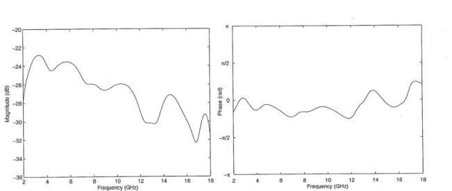
The stored responses were then processed as follows: 1) the ten responses measured at each position were averaged, this reduces any noise present in the system, 2) these average responses are then windowed in the time domain' to select only the direct path, and 3) these windowed responses are then aligned in time by detecting the dominant peak, and averaged to produce a single averaged, windowed response. The time-domain windowing is necessary to remove additional paths caused by reflections in the environment.2 The magnitude and
phase of the resulting response is shown in Fig. 2-6 and the time-domain response is shown in Fig. 2-7. The resulting frequency response can then be used to normalize the frequency responses of the subsequent measured channels. The time-domain response is also used as the template transmit pulse in the channel parameter extraction algorithm (see Sec. 3.4.3).
The antennas also introduce a delay in the captured channel realizations. Removing this delay is very important when using the data to investigate ranging performance. This delay can be estimated by measuring the antenna return loss (i.e., S11 at the antenna input). The magnitude and phase of the return loss are reported in Fig. 2-8. From the measured data, we see that the phase is approximately linear, corresponding to a constant group delay. The group delay of this measurement corresponds to the amount of time it takes a
'A time-domain, raised-cosine window was used with roll-off factor
#=
0.25 and T = 625 MHz.2
__ _ _ __ _ _ __ _ _ __ _ _ __ _ _ _ J -7E~
2 4 6 8 10 12 14 16 18 2 4 6 8 10 12 14 16 18
Frequency (GHz) Frequency (GHz)
Figure 2-6: Magnitude and phase of the average response of the pair of antennas at a distance of 1 m.
-2 -1.5 -1 -0.5 0 0.5 Time (ns)
1.5 2
Figure 2-7: Passband impulse response of the pair of antennas, resulting from the calibration procedure described in Sec. 2.2.2.
signal to travel into the antenna and back out of the input. Thus, half the group delay is a reasonable estimate of the delay introduced by the antennas. Performing a linear best-fit on the phase data yields the following delay estimates:
TTx Ant 0. 824 ns
tRx Ant 0.698
us
- 20
-Transmit Antenna
-5 - - - -Transmit Antenna (linear fit)
0 Receive Antenna
Receive Antenna (linear fit)
-10 - -20 --15 A
~
f/ 4/ \\\~ -40n --20-so-~-25
4 300 -35 - - 120--40 -140--45 - - 160-2 4 6 e 10 12 14 t6 18 2 4 6 8 10 12 14 16 te Frequency (GHz) Frequency (GHz)Figure 2-8: Magnitude and phase of the reflection coefficient (Su1) of the antennas used in
the channel measurement apparatus. Note that the magnitude is approximately less than -10 dB and the phase is nearly linear.
2.2.3 Measurement Accuracy
There are many factors which affect the accuracy of the channel measurement subsystem. The calibration steps discussed above are taken to maximize accuracy of the captured channel realizations, but some sources of error are unavoidable. Below we list these error sources and describe their effect on the measurements.
Antenna response is a function of azimuth and elevation angle
Signal propagation paths originate from the transmit antenna and terminate at the receive antenna at specific azimuth and elevation angles. While the response of the antennas is relatively uniform as a function of azimuth angle, there is a large variation with elevation angle (see Fig. 2-3). Ideally, we would like to correct for the magnitude and phase changes that each of these paths undergo. While it is feasible to measure the antenna response at all possible azimuth and elevation angles, it is difficult to determine the exact angles cor-responding to each propagation path in an experimental setting. This makes it challenging to remove the effect of the antenna on each arriving path. Instead, when removing the response of the antenna from the measurements, we will use the average antenna response measured at a distance of 1 m (estimated using the procedure described earlier).