Numerical Simulation of Pack Ice Forces on Structures: A Parametric Study

Publisher’s version / Version de l'éditeur:

Technical Report, 1999-07

READ THESE TERMS AND CONDITIONS CAREFULLY BEFORE USING THIS WEBSITE.

https://nrc-publications.canada.ca/eng/copyright

Vous avez des questions? Nous pouvons vous aider. Pour communiquer directement avec un auteur, consultez la

première page de la revue dans laquelle son article a été publié afin de trouver ses coordonnées. Si vous n’arrivez pas à les repérer, communiquez avec nous à PublicationsArchive-ArchivesPublications@nrc-cnrc.gc.ca.

Questions? Contact the NRC Publications Archive team at

PublicationsArchive-ArchivesPublications@nrc-cnrc.gc.ca. If you wish to email the authors directly, please see the first page of the publication for their contact information.

For the publisher’s version, please access the DOI link below./ Pour consulter la version de l’éditeur, utilisez le lien DOI ci-dessous.

https://doi.org/10.4224/12328448

Access and use of this website and the material on it are subject to the Terms and Conditions set forth at

Numerical Simulation of Pack Ice Forces on Structures: A Parametric Study

Sayed, Mohamed; Frederking, Robert; Barker, Anne

https://publications-cnrc.canada.ca/fra/droits

L’accès à ce site Web et l’utilisation de son contenu sont assujettis aux conditions présentées dans le site LISEZ CES CONDITIONS ATTENTIVEMENT AVANT D’UTILISER CE SITE WEB.

NRC Publications Record / Notice d'Archives des publications de CNRC:

https://nrc-publications.canada.ca/eng/view/object/?id=9f96537b-cf0f-4499-82bc-9e679bddcecb https://publications-cnrc.canada.ca/fra/voir/objet/?id=9f96537b-cf0f-4499-82bc-9e679bddcecb

Mohamed Sayed, Robert Frederking and Anne Barker

Technical Report HYD-TR-041 PERD/CHC Report 9-80

A PARAMETRIC STUDY

Mohamed Sayed, Robert Frederking and Anne Barker Canadian Hydraulics Centre

National Research Council of Canada Ottawa, Ont. K1A 0R6

Canada

Technical Report HYD-TR-041

ABSTRACT

A numerical model of pack ice interaction with offshore structures is presented. The model is based on using a Particle-In-Cell (PIC) approach to advect the ice cover, and a Mohr-Coulomb plastic yield criterion to describe ice properties. The Zhang-Hibler (1997) numerical scheme is used to solve the momentum equations. A parametric study was conducted in order to determine the influence of shape of the structure, ice thickness, ice properties, and velocity on the resulting ice forces.

TABLE OF CONTENTS

ABSTRACT ... i

TABLE OF CONTENTS ... ii

TABLE OF FIGURES... iii

1. INTRODUCTION ...2 2. THE MODEL ...4 2.1 Overview...4 2.2 Governing Equations ...5 2.3 Numerical Approach ...7 3. TEST CASES...8 4. PARAMETRIC STUDY ...14 5. CONCLUSION ...19 6. ACKNOWLEDGEMENTS ...19 7. REFERENCES ...20 APPENDIX A...22

TABLE OF FIGURES

Figure 1 The staggered grid...7

Figure 2 Schematic of structure and numerical grid...9

Figure 3 Total ice force in x-direction on 100 diameter structure, h=1m, V=0.5 m/s and f=40° ...10

Figure 4 Total ice force in y-direction on 100 diameter structure, h=1m, V=0.5 m/s and f=40° ...10

Figure 5 Ice concentration (a) 60 s and (b) 120 s into the simulation of Run_1, h=1m, V=0.5 m/s and f=40° ...11

Figure 6 Normal stress in x-direction (a) 60 s and (b) 120 s into the simulation of Run_1, h=1m, V=0.5 m/s and f=40°...12

Figure 7 Velocity field (a) 60 s and (b) 120 s into the simulation of Run_1, h=1m, V=0.5 m/s and f=40° ...13

Figure 8 Total force for structures of various shapes, h=1m, V=0.5 m/s and f=40°...15

Figure 9 Total force versus ice thickness for circular structure ...16

Figure 10 Total force versus sin(f) for circular structure ...16

NUMERICAL SIMULATION OF PACK ICE FORCES ON

STRUCTURES: A PARAMETRIC STUDY

1. INTRODUCTION

Ice forces on structures in drifting pack ice are a concern for offshore petroleum production operations off the East Coast of Canada. Methods for estimating those forces, however, remain uncertain. Empirical formulas (e.g. Korzhavin, 1971) have so far been extensively used for design purposes. The pervasiveness of such formulas is the result of their excessive simplicity and the lack of more rigorous methods. However, the simplicity of empirical formulas encompasses gross inaccuracies, which usually produce high estimates of ice forces. For example, the empirical formulas cannot account for specific geometries of structure and ice features, inertial effects, details of ice properties, interaction modes, and forcing conditions.

The complexity of ice-structure interaction also poses several difficulties to numerical modelling. Many interaction scenarios include discontinuities (e.g. in stress and velocity fields), moving and free boundaries, propagation of large cracks, and large deformations. Other less severe difficulties include complex ice rheology and transient behaviour. Consequently, most traditional approaches of numerical modelling had limited success when used to examine ice-structure interaction.

A number of approaches for numerical modelling of ice-structure interaction have been pursued. We only refer to a few recent relevant publications here, which include several references to the available literature. One class of models is based on finite element solutions and continuum constitutive equations. For example, Sand and Horrigmoe (1998) developed a plasticity solution for forces on sloping structures. Another study by Choi and Hwang (1998) used a continuum damage criterion to estimate indentation forces. In order to deal with discontinuities and large cracks, discrete element approaches were used. These approaches include work by Sayed (1997), Katsuragi et al. (1997 and 1998), and Sayed and Timco (1999). The results of those studies show that considerable details of deformation processes can be obtained, albeit at substantial computational cost.

The present study is based on a Particle-In-Cell (PIC) approach, combined with a viscous plastic ice rheology. The PIC model is semi-Lagrangian. It is based on using discrete particles to model ice advection, while solving the momentum equations over an Eulerian grid. The use of discrete particles reduces numerical diffusion, and improves the accuracy of modelling ice boundary conditions. At the same time, the use of an Eulerian grid makes it possible to utilize an implicit

numerical solution scheme for the momentum equations, which substantially increases the computational efficiency.

Several of the ideas used in the present model were originally developed for ice forecasting, at larger scales than ice-structure interaction problems. The viscous plastic formulation that numerically approximates the rigid-plastic behaviour was first developed by Hibler (1979). Flato (1993) implemented a PIC model in an ice forecasting program, and showed that it improves the accuracy. Finally, the present implicit numerical solution of the momentum equations follows an efficient scheme devised by Zhang and Hibler (1997). The present model is adapted from an operational ice forecasting model developed by Sayed and Carrieres (1999). A notable difference, though, is the use of the Mohr-Coulomb yield criterion in the present model instead of the elliptical yield envelope of Hibler (1979).

In summary, the PIC approach was chosen in the present work because it has the following advantages:

• The use of particles to model ice cover geometry and advection makes it possible to model discontinuities and moving boundaries (e.g. ice edges), and reduces numerical diffusion which, for example, allows accurate determination of high pressure zones and modelling of variations in ice thickness and concentration.

• The implicit numerical scheme is much more efficient than explicit methods, which must be used for discrete element methods. For example, the time steps used in the present project range from 0.05 s to 0.2 s. An explicit numerical solution would require a time step of the order of 10-5 s. The ratio between those values of time steps is approximately proportional to computer running time. The relatively high efficiency of the PIC approach makes it possible to model relatively large problems.

• The rheology is based on continuum formulation. This allows the use of familiar models such as the Mohr-Coulomb criterion. Thus, model predictions can be directly compared to other calculation methods and extensive design experience that are based on such continuum rheologies.

This report will briefly describe the numerical model and its adaptation to calculate ice forces resulting from pack ice interacting with structures. The model is next used to conduct a parametric study of the effect of factors such as structure shape, ice thickness, velocity, and pack ice properties on global ice forces.

2. THE MODEL

2.1 Overview

For the Particle-In-Cell (PIC) approach, the ice cover is conceptually represented by discrete particles that are individually advected. The term advection is used here to refer to integrating a particle’s velocity with respect to time, and thus determining the new position (or coordinates). Therefore, the approach can be viewed as a hybrid method. Particles are used to model advection and keep track of ice thickness and concentration (or area coverage). The momentum equations, however, are solved over a fixed (or Eulerian) grid. Continuum equations are also used to describe the rheology of the ice.

In the two-dimensional PIC formulation, each particle is considered to have an area and a volume. The area of a particle can decrease if the pressure exceeds a certain limit (i.e. ridging pressure). The volume, however, remains constant. Thus, if a particle is subjected to relatively high pressures, its area may decrease, and its thickness would correspondingly increase (constant volume = area x thickness). Note that the particles are not actual ice floes, but computational constructs.

At each time step, the areas of the particles are mapped to a fixed grid; i.e. the areas of the particles are converted to continuum ice concentration values (area of ice/ total area) for each node of the grid. Similarly, the thicknesses of the particles are converted to continuum ice thickness values at the nodes of the grid. Such mapping from the particles to the fixed grid is done using a weighting function. Thus, when calculating ice concentration for a node in the fixed grid, particles closer to the node are given higher weight than those farther away from the node.

Once values of ice concentration and thickness are determined at each node of the fixed grid, the continuum momentum and rheology equations are solved over that grid. Those continuum equations can thus be solved in an efficient way. The use of a fixed grid makes it possible to employ implicit numerical methods, which are efficient. The time steps can be very large compared to explicit formulations that must be used, for example, in discrete element methods. In the present model, the numerical method of Zhang and Hibler (1997) is used because of its efficiency.

The solution of the momentum and rheology equations gives velocity values at the nodes of the fixed grid. Those velocities are mapped from the nodes to the particles in a manner similar to that discussed above. The particles are then advected to new positions.

2.2 Governing Equations

The governing equations consist of:

• Continuum linear momentum equations.

• Continuum rheology, which is represented here by a viscous plastic model of Mohr-Coulomb yield criterion.

• Mapping functions to convert particles’ areas and thicknesses to continuum values on the fixed grid, and to convert velocities at the grid nodes to velocities for each particle.

The momentum equations are expressed as

w a ice dt u d u u dt u d h σ τ τ ρ r r r r r r + + ⋅ ∇ =       _{+ ∇} (2.1) where ρice is the ice density, h is the ice thickness, u

r

is the velocity vector, σ is the stress tensor, and τr_a

and τr_w

are the air and water drag stresses. The air and water drag stresses are given by the following quadratic formulas

a a a a a

c

U

U

r

r

r

ρ

τ =

(2.2) and

(

u

)

u

c

_{w w w w} w

r

r

r

r

r

-U

-U

ρ

τ =

(2.3)

where ca and cw are the air and wind drag coefficients, Ua r

is wind velocity, Uw r

is water velocity, and ρa and ρw are the air and water densities, respectively.

Eq.(2.2) assumes that ice velocity is small compared to wind velocity. The stress-strain rate relationship is given by

•

+

−

=

_{ij ij} ij

p

δ

η

ε

σ

2

(2.4)

where ε•_ij is the strain rate, p is the mean normal stress, and η is the shear viscosity.

The mean normal stress, p, is usually considered to increase with increasing ice compactness, A (area of ice/total area). We use here a formula analogous to that of Hibler (1979). Note, however, that p is different from the strength P used by Hibler (1979) by a factor of two.

(

(1 )

)

exp * A C h P P= _ice − − (2.5)

The Mohr-Coulomb criterion is introduced by giving the shear viscosity, η, the following value

(

)

∆ + = φ φ η ccot p sin (2.6)

where c is the cohesion and f is the angle of internal friction. The strain rate ∆ is given by         − = ∆ • • , •₀ 2 1 max

ε

ε

ε

(2.7)

where ε•₁ and ε•₂ are the principal strain rates and ε•₀ is a threshold strain rate. For relatively large strain rates, ∆> ε•0, the rheology is plastic and the yield

criterion is satisfied. At small rates of deformation, however, the shear viscosity becomes constant, and the corresponding rheology would be viscous. A very small threshold strain rate (typically ε•0= 10

-20

s-1) is used in order to maintain a predominantly plastic deformation.

The above formulation allows for tensile normal stresses. A tension cut-off value is further introduced in the model. If a normal stress exceeded that limit, the viscosity coefficient, η, is adjusted such that the maximum tensile stress is set equal to the tensile strength of ice.

The preceding set of equations, together with PIC advection, is sufficient to determine the stresses, velocities, and configuration of the ice cover through its interaction with a structure. The PIC scheme and the interpolation functions used to map variables between the particles and fixed grid are discussed in Appendix A.

2.3 Numerical Approach

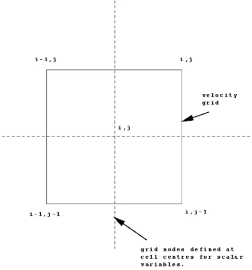
The solution is implemented using a staggered grid as illustrated in Figure 1. The velocity components are defined at the corners of the velocity grid. All scalar values (pressure, viscosities, thickness and concentration) are defined at the centres of the grid cells.

Figure 1 The staggered grid.

Starting from a given initial configuration, the numerical solution of the above governing equations updates the velocities, pressures, thicknesses, and concentrations at each time step. The main logic of the solution consists of the following steps:

• Advect the particles to new positions (Appendix A).

• Determine the thickness and concentration values by interpolating the area and volume of the particles to the scalar grid (Appendix A).

• Correct the thickness and concentration values by adjusting concentrations higher than unity. Next, correct the area and thickness of each particle (Appendix A).

• Calculate the pressures on the scalar grid using Eq.(2.5).

• Solve the momentum equations Eq.(2.1). This is the major part of the solution.

• Determine particle velocities by interpolating values from the velocity grid (Appendix A).

The implicit numerical solution of the momentum equations follows the approach of Zhang and Hibler (1997). Details of the solution method are too lengthy to be given here. In addition to the above reference, the solution method was also discussed by Sayed (1998).

3. TEST CASES

Four shapes of the structure were investigated in the study: circular, square, diamond and octagonal. The width of all four structures perpendicular to the ice movement direction was the same (that is 100m). A fifth structure, the square rotated 45o, was also examined. Its width, normal to the ice movement direction, was 141 m. These structures were selected to represent a range of generic structure shapes which offshore production structures might take. As mentioned in the introduction, numerical simulation lends itself to modelling geometries that are considerably more complex, such as rectangles, multi-leg structures, and ship-bow shapes. There is a wide range of such structures and they are best dealt with on a case by case basis.

The three pack ice parameters that were varied in the study included thickness, velocity, and rheology. The rheology assumed for the pack ice was based on the Mohr-Coulomb yield criterion of a cohesionless material, so the only strength variable was the angle of internal friction, f. In the formulation of the problem, it is assumed that the pack ice behaves as a continuum, thus floe size does not appear explicitly in the formulation. To make this assumption of continuum behaviour, however, floe size should be smaller than about 20% of the structure size. Floe size is a factor that has been observed to effect ice forces, so this is a factor that eventually has to be taken into account. Since the only pack ice strength property available in this formulation is the angle of internal friction, f, this parameter will thus account for the overall ice cover properties, the effects of floe size, and interlocking and friction between floes. The other ice factor that characterizes the pack ice is the concentration. For this study, an initial value of 0.8 was assumed at the start of each simulation run.

The results of a base case will be presented in detail to demonstrate the insights the simulation can deliver. A schematic of the structure, in this case circular, and the calculation grid is presented in Figure 2. The grid is 50 nodes wide and 130

nodes long. Each grid cell is 10 m, thus 11 grid points define the structure width of 100 m. The base case was for 1 m thick ice, with an internal friction angle of 40°, and a velocity of 0.5 m/s. The pack ice cover initially extends from node #30 to node #130. The area from node #0 to node #30 was left empty to provide space for the pack ice to move to the left, unhindered in the x-direction. Figure 3 is a time series of the force on the structure in the x-direction (direction of ice motion), for base case conditions. This force was calculated by taking the average of the stresses in the x-direction on a 100 m long line along the x-axis node #51 from y-axis node #20 to #30. It is also possible to determine the force component acting on the structure in the y-direction, as shown in Figure 4. It can be seen that the maximum lateral force is less than 5 % of the force in the direction of ice motion.

10 20 30 40 50 60 70 80 90 100 110 120 130

Node Number - x direction 10 20 30 40 50 N ode Num ber - y di rec tio n

0 0.1 0.2 0.3 0.4 0.5 0 50 100 150 200 Time (s) Force (MN )

Figure 3 Total ice force in x-direction on 100 diameter structure, h=1m, V=0.5 m/s and f=40°

Figure 4 Total ice force in y-direction on 100 diameter structure, h=1m, V=0.5 m/s and f=40° -0.02 0 0.02 0 50 100 150 200 Time (s) Forc e in y -direc tion (M N)

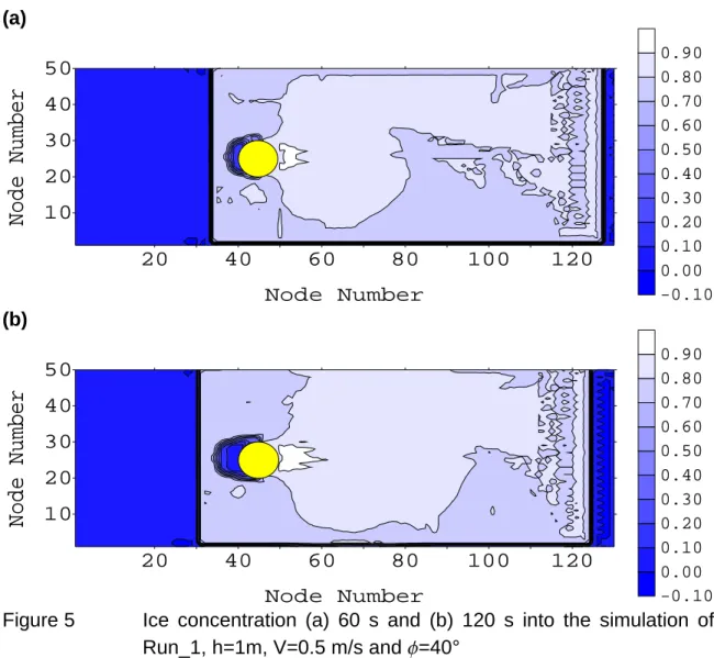
The results of the simulation determine the evolution of the stress, velocity, concentration, and thickness. As an example, results from the base case (Run_1) will be presented. Figure 5 is a plot of the concentration after 60 s and 120 s into the simulation. Two features are apparent in this figure. Firstly, a high concentration area in front of the structure can be seen developing at 60 s and becoming larger by 120 s. These are qualitative observations that agree with field observations, and hence lend confidence to the simulation. Secondly, a wake can seen developing downstream from the structure. Figure 6 is a plot of the distribution of normal stress in the x-direction at times 60 s and 120 s, with compressive stress shown positive. The development and expansion of an area of high stress in front of the structure is apparent. Figure 7 shows plots of the velocity vectors at 60 s and 120 s. A zone of slowing velocity, extending about 2 diameters ahead of the structure, can be seen at 60 s. By time 120 s, this zone has extended to about two and a half structure diameters, and a wake is visible downstream from the structure.

(a) 20 40 60 80 100 120 Node Number 10 20 30 40 50

No

de Nu

mber

-0.10 0.00 0.10 0.20 0.30 0.40 0.50 0.60 0.70 0.80 0.90 (b) 20 40 60 80 100 120 Node Number 10 20 30 40 50

No

de Nu

mber

-0.10 0.00 0.10 0.20 0.30 0.40 0.50 0.60 0.70 0.80 0.90

Figure 5 Ice concentration (a) 60 s and (b) 120 s into the simulation of Run_1, h=1m, V=0.5 m/s and f=40°

(a)

20

40

60

80

100

120

Node Number

10

20

30

40

50

Node

Num

ber

-3000 Pa -1000 Pa 1000 Pa 3000 Pa 5000 Pa 7000 Pa 9000 Pa (b)

20

40

60

80

100

120

Node Number

10

20

30

40

50

Node

Num

ber

-3000 Pa -1000 Pa 1000 Pa 3000 Pa 5000 Pa 7000 Pa 9000 Pa

Figure 6 Normal stress in x-direction (a) 60 s and (b) 120 s into the simulation of Run_1, h=1m, V=0.5 m/s and f=40°

(a)

30

40

50

60

70

80

90

100 110 120

Node Number

10

20

30

40

50

No

de

N

u

mbe

r

(b)

30

40

50

60

70

80

90

100 110 120

Node Number

10

20

30

40

50

N

ode

Nu

mbe

r

Figure 7 Velocity field (a) 60 s and (b) 120 s into the simulation of Run_1, h=1m, V=0.5 m/s and f=40°

4. PARAMETRIC STUDY

An extensive set of runs was done in order to determine the role of geometry of the structure, ice cover properties and ice velocity. Five different structures were examined. The following pack ice properties and conditions were used:

- Ice thickness, h = 0.5, 1, 2 and 4 m

- Angle of internal friction, f = 35, 40 and 45o

- Ice cover velocity, V = 0.1, 0.2 0.5 and 1 m/s

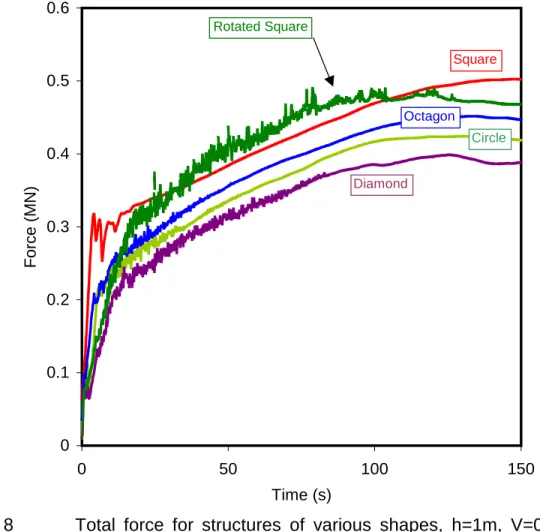
The results for the base case of the five different structures are compared in Figure 8. For structures with a 100m wide face perpendicular to the direction of ice motion, progressively larger maximum forces were predicted for a diamond, circular, octagonal and square shape. The maximum force values are summarized in Table 1. The trend of ice force with structure shape generally follows the trend observed elsewhere in the literature (e.g. Korzhavin, 1962). One result that is surprising, is the comparison of the force on the square and the rotated square. Note that there is a slight decrease in total force from the square to the rotated square, even though the width of the structure presented to the ice movement direction has increased from 100m to 141m.

0 0.1 0.2 0.3 0.4 0.5 0.6 0 50 100 150 Time (s) Force (MN) Square Diamond Circle Octagon Rotated Square

Figure 8 Total force for structures of various shapes, h=1m, V=0.5 m/s and f=40°

Table 1 Maximum force values for base case conditions.

Structure Maximum Force (MN) Normalized Force

Square, 100 m wide 0.502 1.00

Octagon, 100 m wide 0.452 0.90

Circle, 100 m wide 0.424 0.84

Diamond, 100 m wide 0.399 0.79

Rotated Square, 141 m wide 0.490 0.98

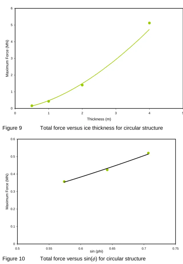
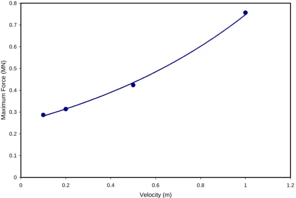
The next aspect of the parametric study was to examine the effects of ice thickness, internal friction angle and velocity. Each factor was examined in turn, and an empirical expression was fit to the data. The effect of ice thickness on the maximum force on a circular structure is plotted in Figure 9. Note that similar trends were seen for the other structure shapes. The influence of the angle of internal friction, f, and velocity, V, are illustrated in Figures 10 and 11.

0 1 2 3 4 5 6 0 1 2 3 4 5 Thickness (m) Maximum Force (MN)

Figure 9 Total force versus ice thickness for circular structure

0 0.1 0.2 0.3 0.4 0.5 0.6 0.5 0.55 0.6 0.65 0.7 0.75 sin (phi) Ma xi mu m F o rce (MN )

0 0.1 0.2 0.3 0.4 0.5 0.6 0.7 0.8 0 0.2 0.4 0.6 0.8 1 1.2 Velocity (m) Max imum F o rc e (MN )

Figure 11 Total force versus ice velocity for circular structure

The dependence of the total force on the structure, Fc, on each parameter is

given by the following curve-fit equations. The role of ice thickness, h, is represented by 67 . 1

h

F

_c

∝

(4.1)

where pack ice thickness, h, is in meters. The effect of the internal friction effect, f, is given by

( )

8 . 1 0 40 sin sin       ∝ φ c F (4.2)

Finally, the expression for velocity, V, dependence is given by

(

V

)

F_c=0.25exp1.07 (4.3)

where V is velocity in m/s, for the base case of h = 1 m and f = 40o. Combining these three expressions, the following empirical relation is obtained

(

)

[

][ ]

_{( )}

0 1.8 67 . 1 40 sin sin 07 . 1 exp _      =S V h φ F_c (4.4)

where S is a coefficient which accounts for the shape of the structure. Note that this is a dimensional equation and care must be taken to ensure correct units are applied for each input parameter. In addition, being an empirical expression, caution must be exercised in extrapolating beyond the ranges for which the original parametric study was conducted. Equation (4.4) does not take into account structure width since all calculations were for a 100 m width of structure, except for the rotated square. The shape coefficient, S, is given in Table 2. Table 2 Shape coefficient, S to be applied in Equation (4.4)

Structure Shape Shape Coefficient, S

Square, 100 m wide 0.30

Octagon, 100 m wide 0.27

Circle, 100 m wide 0.25

Diamond, 100 m wide 0.24

Rotated Square, 141 m wide 0.29

A search was made of the literature to see whether there were any full-scale data that could be used for validating the predictions of the simulations. Some data were located for ice forces on the Gulf Kulluk, a circular conical drilling unit (Wright, 1999). The Kulluk is about 70 m in diameter at the waterline. Its mooring lines were instrumented so forces on the unit due to drifting pack ice could be determined. Observations of ice conditions were also documented. Wright (1999) abstracted ice force data for various ice conditions. What he describes as “managed ice with good clearance” seems to coincide most closely with the ice properties used for the numerical simulations. This ice condition was for ice floes less than 50 m in diameter, which flowed in a “slurry”-like fashion around the Kulluk. Some of his general observations were that (i) force increased linearly with ice thickness, (ii) no clear velocity effects were discernable up to speeds of 0.5 m/s and (iii) force increased with concentration. Quantitatively the following data were extracted for validation purposes:

• ice conditions

- thickness 2 m

- floe size less than 50 m

- drift speed 0.25 – 0.50 m/s • ice forces

- less than 0.8 to 1.0 MN

Using Equation (4.4), an ice thickness of 2 m, an internal friction angle of 30° and a velocity range of 0.25 – 0.50 m/s, the predicted force ranges from 0.66 MN to 0.86 MN. Further validation will be done in a future study, however, it can be

seen that the numerical simulation force predictions agree well with full-scale data.

5. CONCLUSION

This report has described a new numerical model of ice-structure interaction. The model is based on a PIC scheme for ice advection. This scheme reduces numerical diffusion, can handle the types of boundary conditions encountered in ice-structure interaction problems, and particularly improves the accuracy of predicting ice stresses. The model uses a viscous plastic rheology to approximate a rigid-plastic Mohr-Coulomb yield criterion.

A significant feature of the model is the use of the Zhang-Hibler numerical method to solve the momentum equations. That method leads to substantial improvements in the computational efficiency. Consequently, relatively large problems of practical significance can be examined.

The model was used to conduct a parametric study of pack ice forces on structures of various shapes. The resulting distributions of stresses, ice concentrations, and velocity appear to agree with intuitively expected trends and the available sparse field observations. The roles of ice thickness, ice properties, and velocity were also determined. The results were summarized in the form of empirical equations in order to make them convenient for use by interested readers.

The results of the parametric study show that ice thickness has the most significant influence on the total force, followed by ice cover properties, which are expressed in terms of an angle of internal friction. The shape of the structure appears to have minor effect on the resulting force. We caution, however, that the preceding conclusions should be valid only for the examined range of conditions of pack ice and structure types.

6. ACKNOWLEDGEMENTS

The financial support of the Program on Energy Research and Development (PERD) is gratefully acknowledged.

7. REFERENCES

Choi, K., and Hwang, O.J. (1998). ”Continuum damage modelling for the estimation of ice load under indentation,” Proceedings of the 8th International Offshore and Polar Engineering Conference (ISOPE ‘98), Montreal, Canada, Vol. II, pp.468-475.

Flato, G.M. (1993). “A Particle-In-Cell sea-ice model,” Atmosphere-Ocean, Vol. 31, No. 3, pp. 339-358.

Hibler, W.D.III (1979). “A dynamic thermodynamic sea ice model,” J. Physical Oceanography, Vol. 9, No. 4, pp. 815-846.

Katsuragi, K., Ochi, M., Seto, H., and Kawasaki, T. (1997).”Distinct element simulation of ice sheet failure against offshore structures,” Proceedings of the 7th International Offshore and Polar Engineering Conference (ISOPE ‘97), Honolulu, Vol. II, pp.356-359.

Katsuragi, K., Kawasaki, T., Seto, H., and Hayashi, Y. (1998).”Distinct element simulation of ice-structure interaction,” Proceedings of the 8th International Offshore and Polar Engineering Conference (ISOPE ‘98), Montreal, Canada, Vol. II, pp.395-401.

Korzhavin, K.N. (1971). ”Action of ice on engineering structures,” US Army CRREL Translation TL260, Hanover, NH, USA.

Sand, B., and Horrigmoe, G. (1998).”Simulation of ice forces on sloping structures,” Proceedings of the 8th International Offshore and Polar Engineering Conference (ISOPE ‘98), Montreal, Canada, Vol. II, pp.476-482.

Sayed. M., 1997. Discrete and Lattice Models of Floating Ice Covers, Proceedings of the 7th International Offshore and Polar Engineering Conference (ISOPE ‘97), Honolulu, Vol. II, pp.428-433.

Sayed, M. (1998).”Ice model development: implementation,” Technical Report HYD-TR-036, Canadian Hydraulics Centre, National Research Council, Ottawa, Ontario, Canada, June 1998.

Sayed, M., and Carrieres, T. (1999).”Overview of a new operational ice forecasting model,” Proceedings of the 9th International Offshore and Polar Engineering Conference (ISOPE ‘99), Brest, France, Vol. II, pp.622-627.

Sayed, M., and Timco, G.W. (1999).”A lattice model of ice failure,” Proceedings of the 9th International Offshore and Polar Engineering Conference (ISOPE ‘99), Brest, France, Vol. II, pp.528-534.

Wright, B.D. (1999).”Evaluation of full scale data for moored vessel stationkeeping in pack ice,” Report to the National Research Council on behalf of the Program on Energy Research and Development (PERD) by Brian Wright and Associates, March 1999.

Zhang, J. and Hibler, W.D.III (1997).”On an efficient numerical method for modelling sea ice dynamics,” J. Geophysical Research, Vol. 102, No. C4, pp. 8691-8702.

APPENDIX A

The PIC formulation follows the approach of Flato (1993). The ice cover is discretized into individual particles that are advected in a Lagrangian manner. In this formulation, each particle is considered to have an area and a thickness. For each time step, the particle velocities are determined by interpolating node velocities of an Eulerian grid. Particles can then be advected. The area and mass of each particle are then interpolated back to update the thickness and ice concentration at the Eulerian grid nodes.

A bilinear interpolation function is used to map variables between the particles and the Eulerian grid. For a particle n at location xp, yp, and grid node

co-ordinates (xij, yij), the interpolation coefficients ω would be given by

   − ≤∆ = ∆ − − ∆ = otherwise x x t n x if n j i S x n j i S x t n x x t n x x ij p x x ij p p ij x 0 ) , ( 1 ) , , ( ) , , ( |] ) , ( | [ )) , ( , ( ω (A.1) and    _{− ≤∆} = ∆ − − ∆ = otherwise y y t n y if n j i S y n j i Sy y t n y y t n x x ij p y ij p p ij y 0 ) , ( 1 ) , , ( ) , , ( |] ) , ( | [ )) , ( , ( ω (A.2)

where t is time, and ∆x and ∆y are the grid cell dimensions.

Thus, the particle velocity components, up and vp can be calculated as follows

) , ( )) , ( , ( )) , ( , ( )) , ( ( ), , ( )) , ( , ( )) , ( , ( )) , ( ( j i v t n y y t n x x t n X v j i u t n y y t n x x t n X u p ij y p ij x j i p p ij y p ij x j i p ω ω ω ω ∑ ∑ = ∑ ∑ = (A.3)

where u(i,j) and v(i,j) are the velocity components of the Eulerian velocity grid. Once particles’ velocities are determined, advection of a particle, n at location X, can be expressed as

∫

∆ + ′ ′ ′ + = ∆ + t t t t d t t n t n t t n, ) ( , ) ( ( , ), ) ( X u X X (A.4)

where u is the particle’s velocity vector and ∆t is the time step. According to Flato (1993), the integral in Eq. (A.4) can be approximated by

2 ) ), , ( ( ) , ( , )) , ( ( ) ), , ( ( t t t n t n t t n t d t t n t t t ∆ + = ∆ = ′ ′ ′

∫

∆ + X u X X X u X u * * (A.5)

The updated thickness and concentration are determined at each time step by mapping particles’ areas and volumes back to the Eulerian grid. In the present case, a staggered B-grid is used. Therefore, the thickness and concentration values correspond to a set of nodes different from those used for the velocities. The values of node concentration c(xij, t) are determined as follows

∑

_{∆ ∆} = n ij y ij x ij y x t n A t n x t n x t x c( , ) ω ( ,X( , ))ω ( ,X( , )) ( , ) 1 (A.6) where A(n,t) is the area of particle n. The values of node thickness are then calculated as follows

∑

_{∆ ∆} = n ij ij y ij x ij y x t x c t n V t n x t n x t x h ) , ( 1 ) , ( )) , ( , ( )) , ( , ( ) , ( ω X ω X (A.7)

where V(n,t) is the volume of particle n.

The resulting concentration and thickness are further modified to account for ridging, which may occur if the ice cover converges. If the concentration at a node, according to Eq. (A.6), is larger than unity, its value is adjusted to one. The thickness at that node is also increased to conserve the volume of ice. Such a correction of concentration and thickness is mapped back to the particles. A factor F (larger than or equal to1) is used to reduce the area and increase the thickness of each particle. The value of F is determined by

{

( , ),1

}

max ) , ( ~ 1 ), , ( ~ )) , ( , ( )) , ( , ( max ) , ( t x c t x c t x c t n x t n x t n F ij ij ij ij y ij x j i =     ∑∑ = ω X ω X (A.8)